
Robust Sliding Mode Control of Air Handling Unit for Energy Efficiency Enhancement


Abstract
:1. Introduction
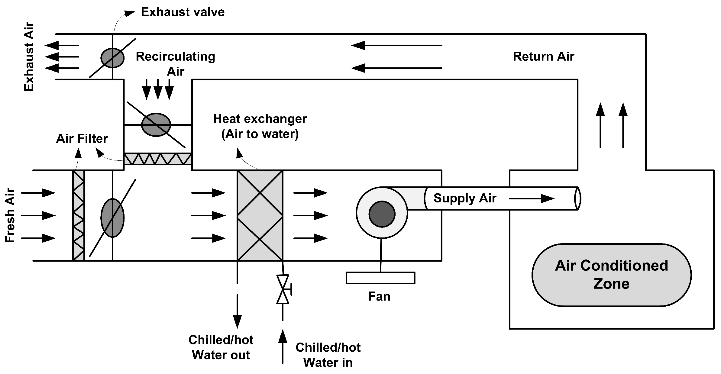
2. Air Handling Unit
- 75% of recirculated air is mixed with 25% of fresh air and the rest is exhausted.
- After passing through the filter, this air gets conditioned in the heat exchanger.
- The conditioned air (supply air) enters the thermal zone by supply fan.
- After offsetting the latent (humidity) and sensible heat (actual heat), the return air is drawn out by a duct where 25% of recirculated air is exhausted via exhaust dampers.
Dynamic Modeling
- There should be no air leakage in the duct work except at exhaust air dampers.
- Air flow is homogeneous.
- Ideal gasses must be employed.
- Zone air pressure is independent of air speed variations.
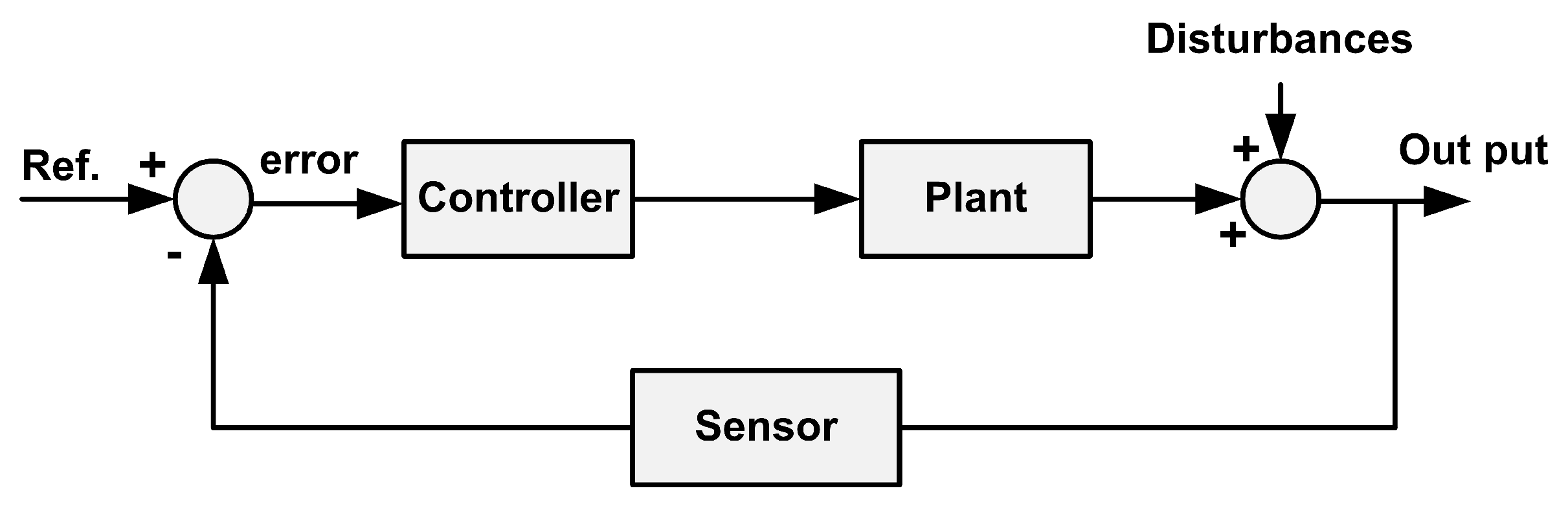
3. Controller Design
3.1. PID Controllers
Tuning of PID Controllers
- Transform the PID controller into a P by adjustment of and . At first, set pick up to . Close the loop in programmed mode for the controller.
- Increase unless there are maintained motions in the signs in the control system. This esteem is signified a definitive gain, .
- Measure a specific period of the maintained oscillations.
- Figure the controller parameter esteems as per Table 3, and utilize these parameter esteems in the controller.
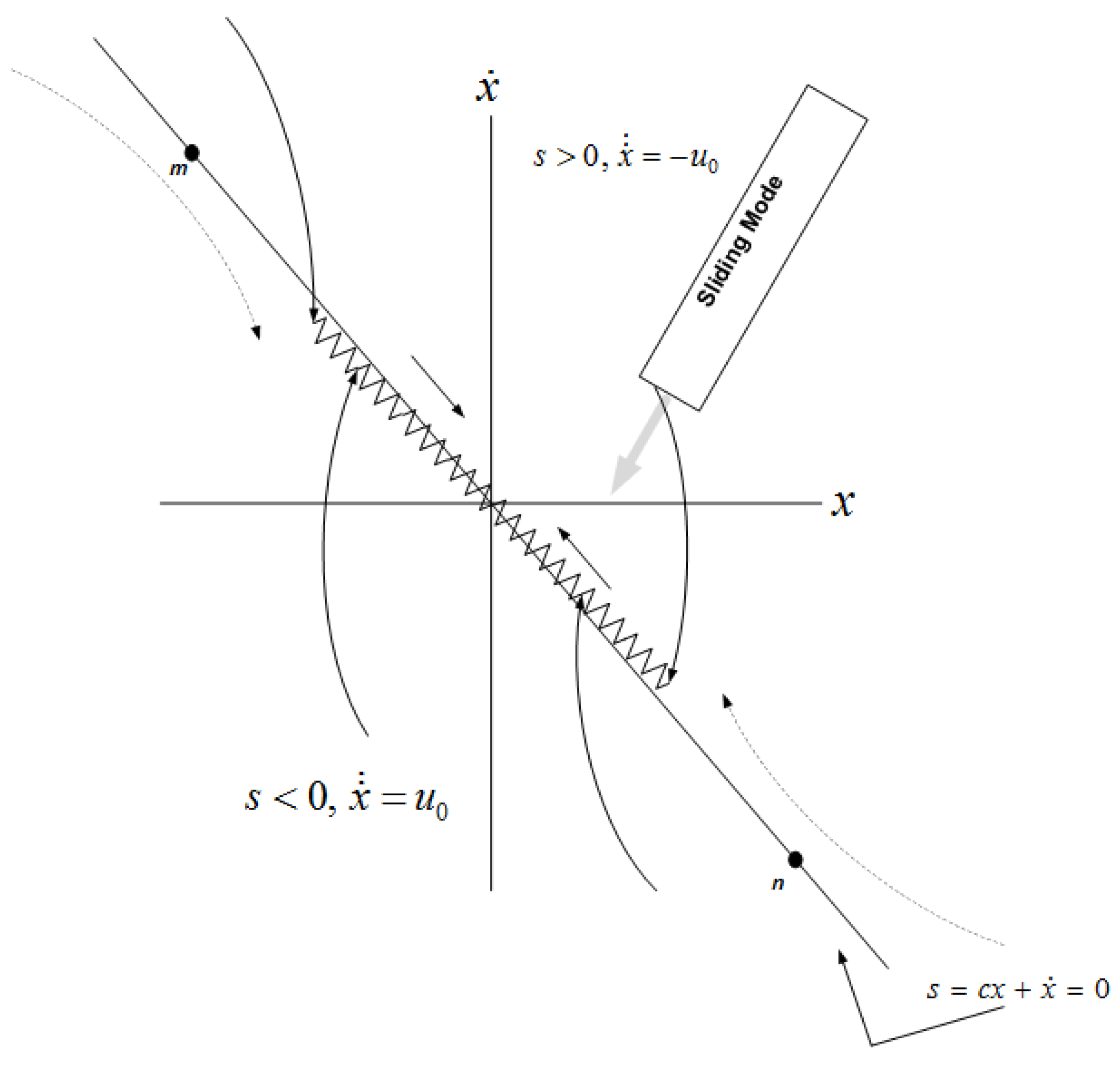
3.2. Sliding Mode Control
- The direction of trajectories is towards .
- The trajectories have a place with the switching and can’t leave it.
- Once sliding mode begins, additional movement is administered by the equation .
3.3. Selection of SMC over PID
- Typically, the HVAC frameworks are nonlinear with variations in parameters. Henceforth, utilizing PID control strategy may hamper system stability because of the conceivable over linearization of the system. Then again, a sliding mode control doesn’t overlook nonlinearity.
- The capability of the framework is dependent on the load. On account of displaying miscalculation, the sliding mode control provides a deliberate approach to maintain the stability and in addition the coveted reliable performance.
- The sliding mode control implementation on hardware is simple. In the microcontroller, it needs less numerical and computational calculations. The standard protocols are promptly perfect with it, for example, Modbus and the Ethernet/IP, RS-232.
- For the situations, where accuracy and stability are required, SMC requires altogether less maintenance and gear costs.
3.4. SMC Design
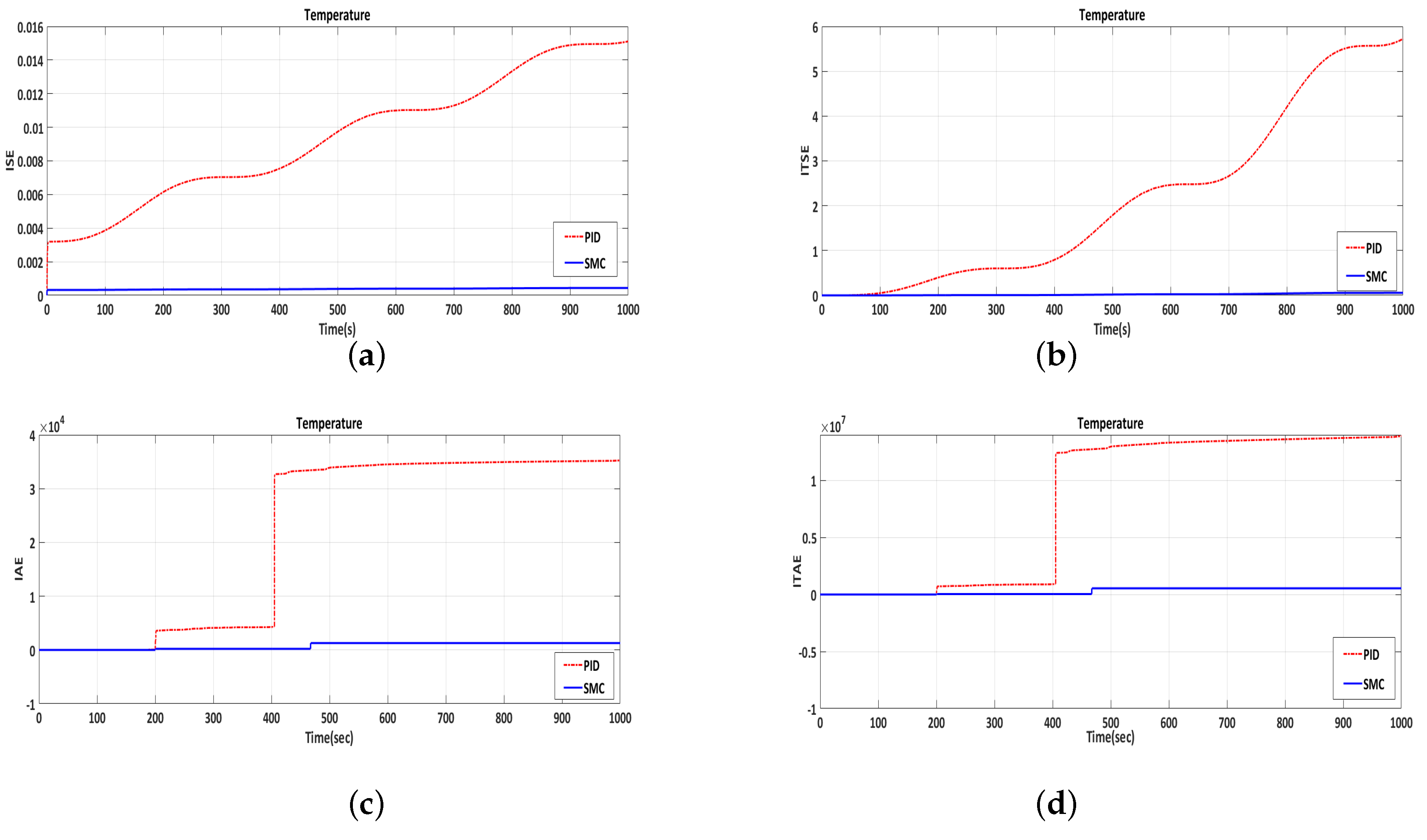
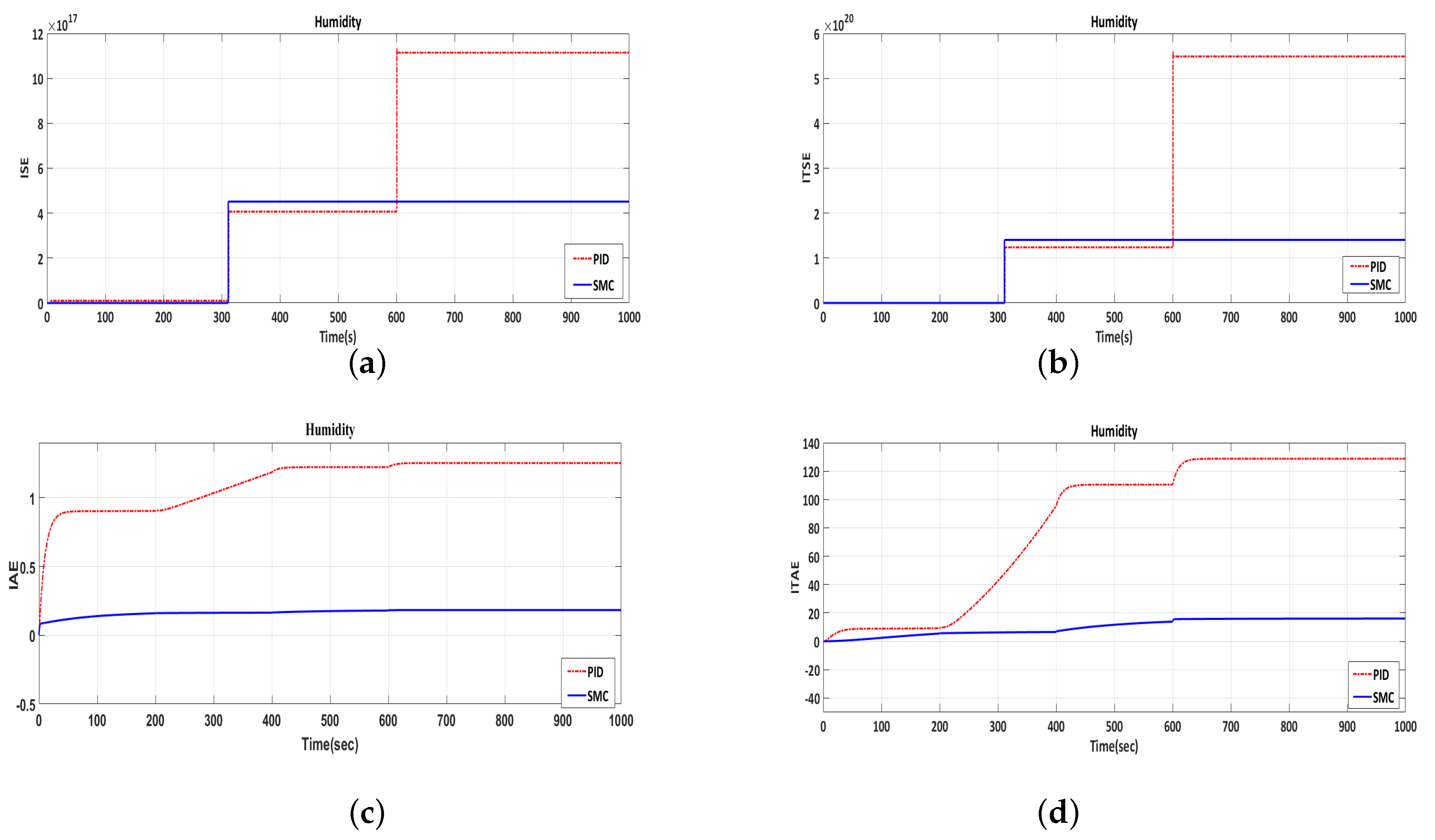
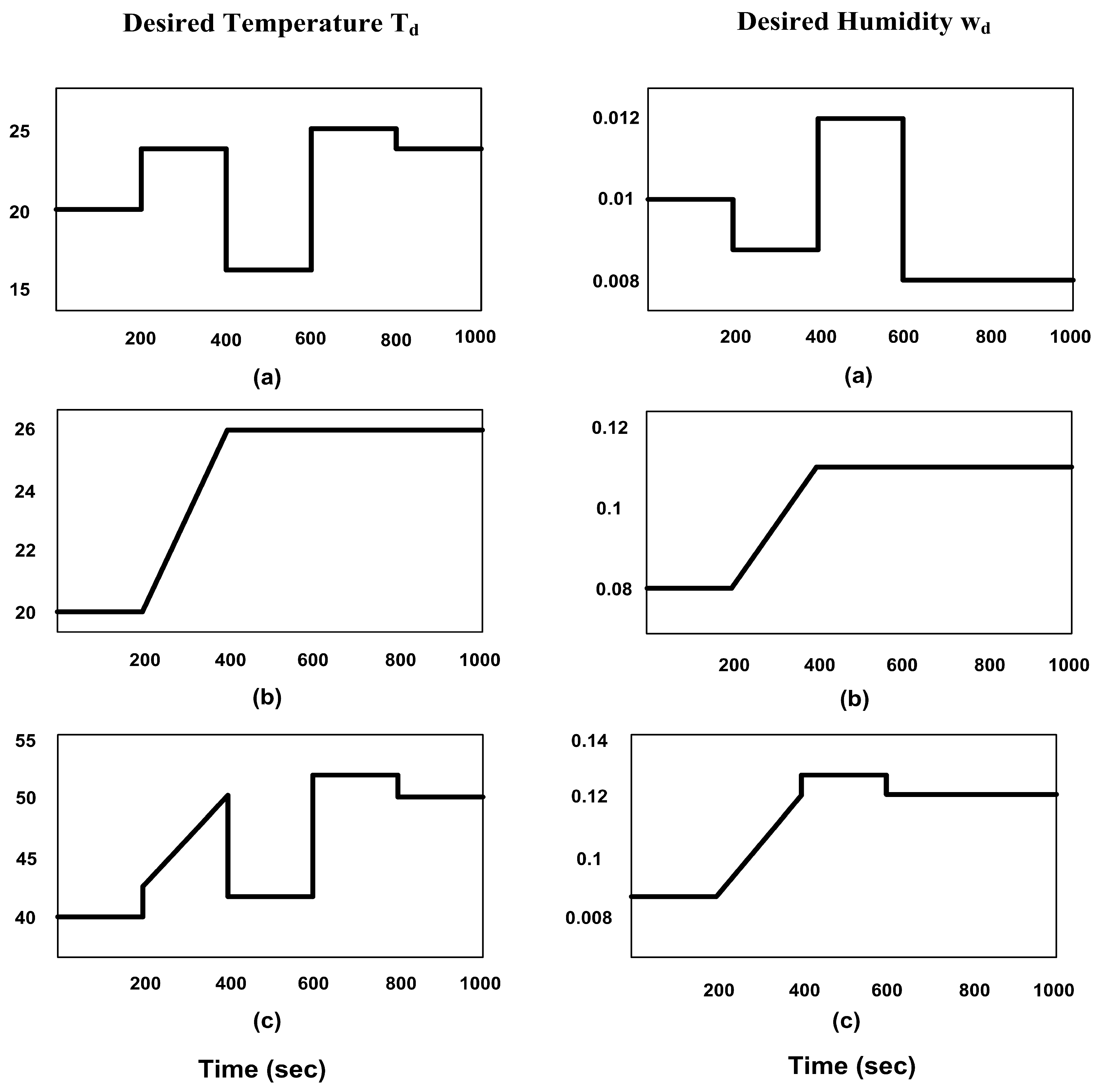
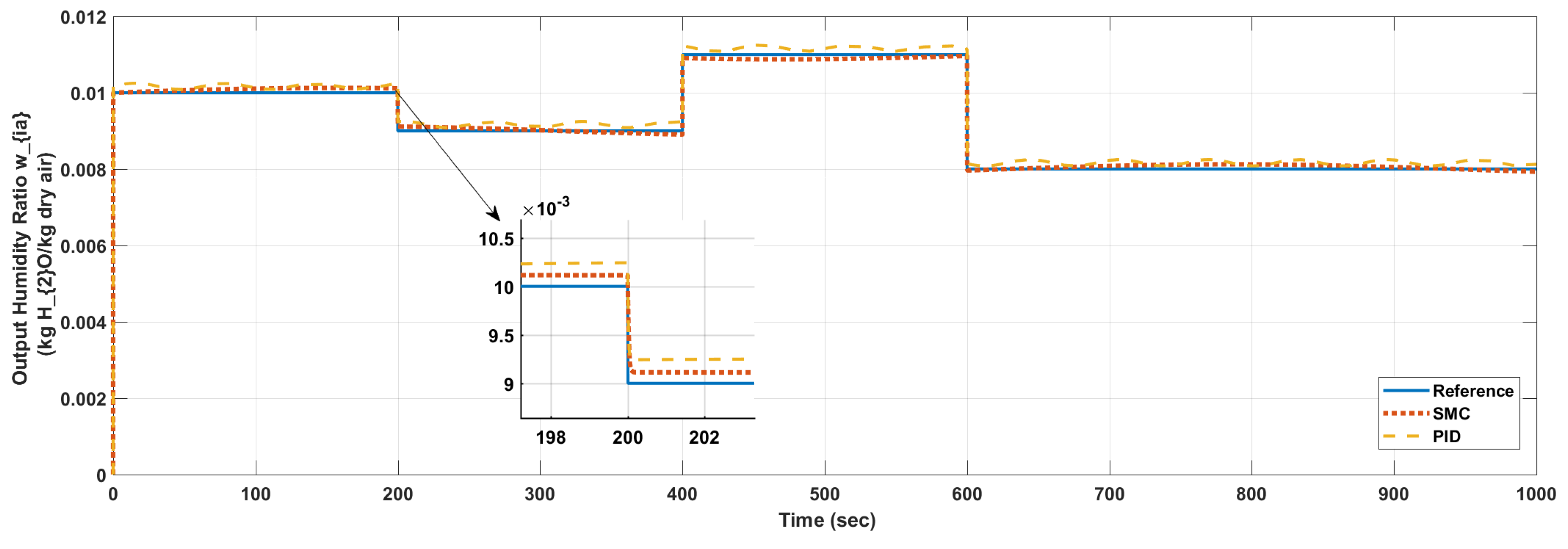
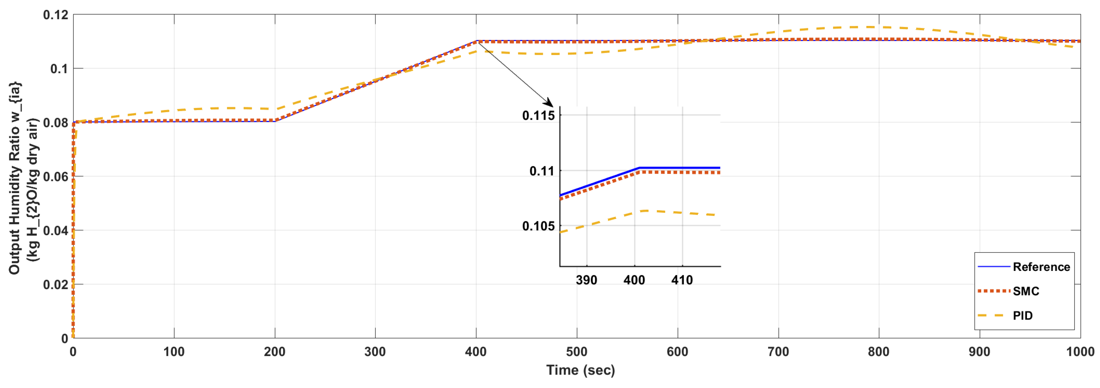
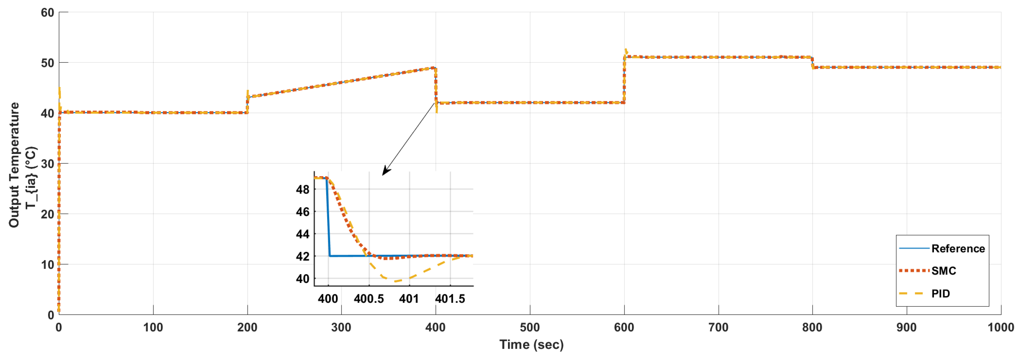
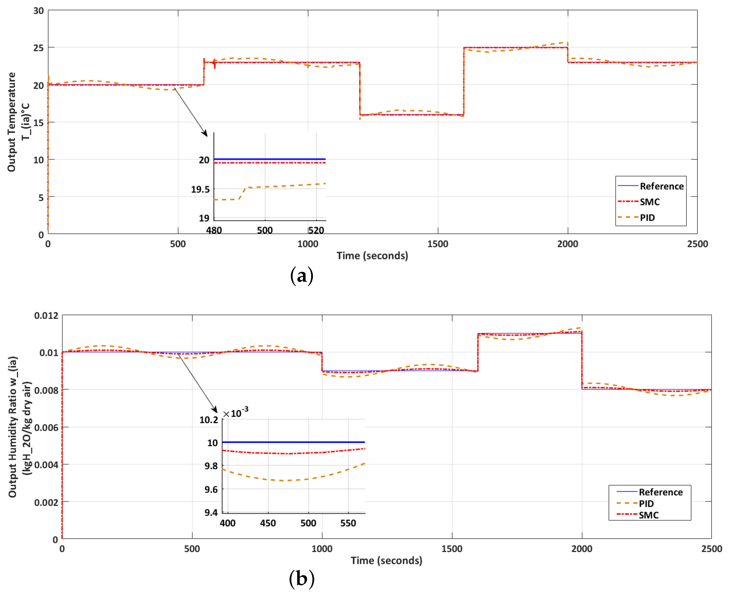
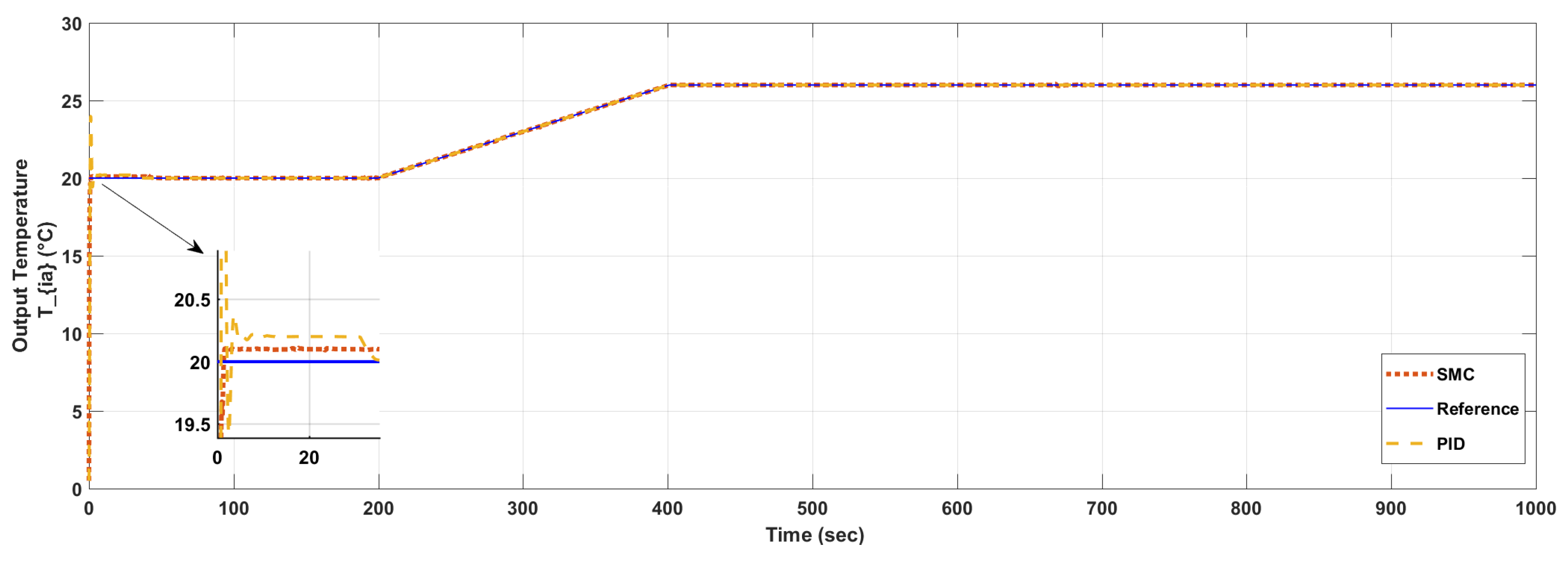
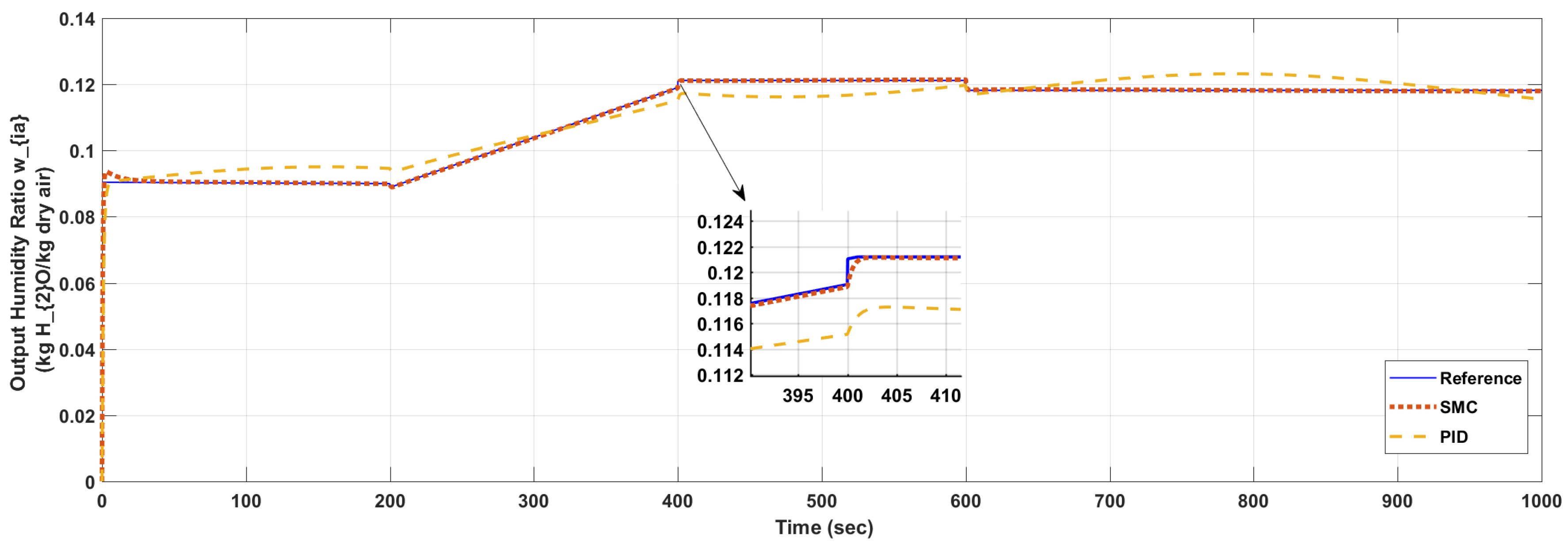
4. Results
5. Conclusions
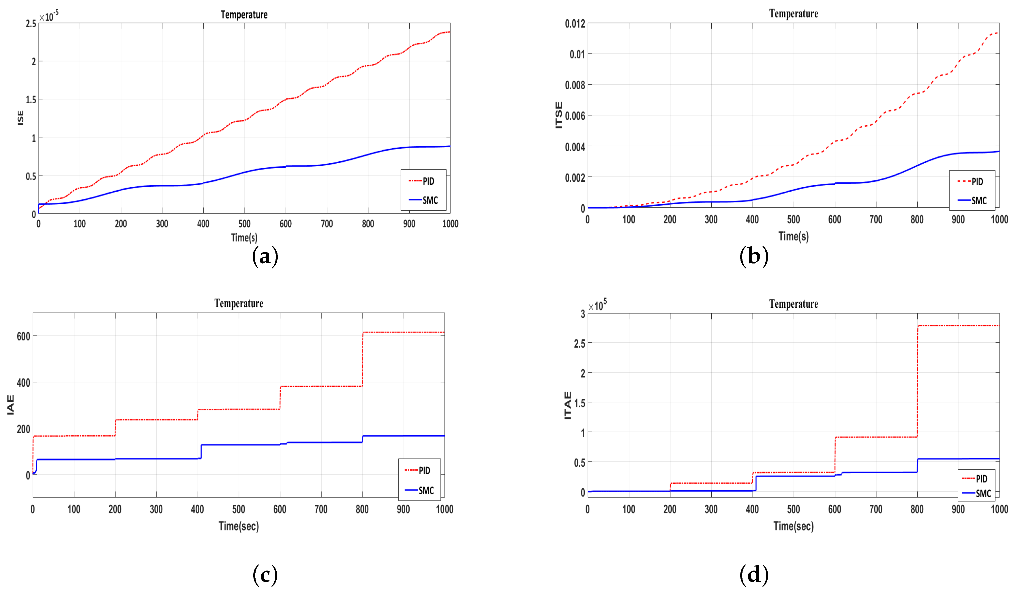
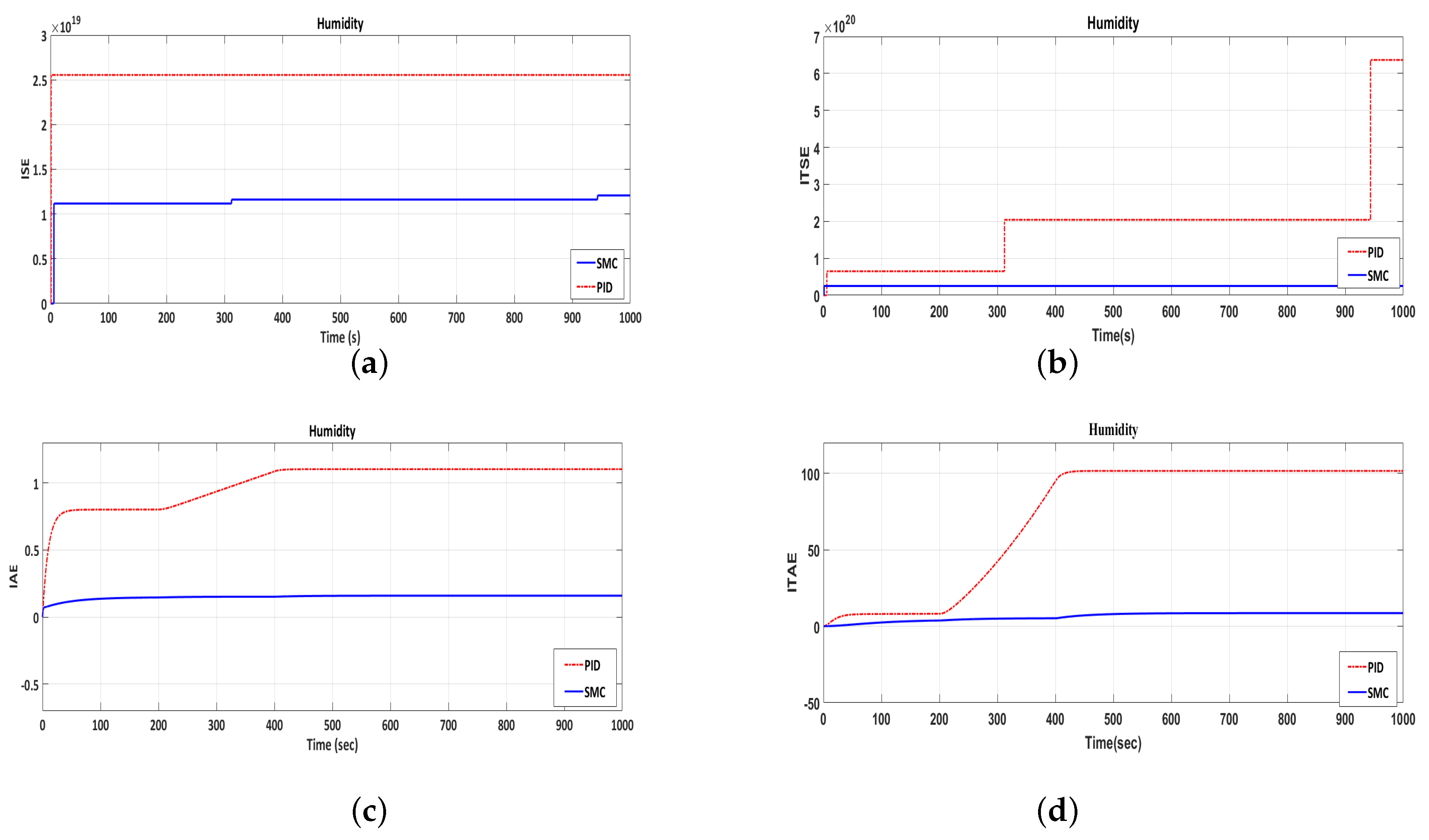
- Sliding mode control ensures robustness by tracking the setpoints perfectly (low overshoot and less time for convergence) in the presence of uncertainties, but PID shows high oscillation as compared to SMC in tracking the setpoint objectives.
- Sliding mode based controller design for AHU contributes to lower energy consumption due to less time for convergence and less overshoot contributing to lowering the air and the water flow requirement.
- The oscillatory behavior of PID controller is disadvantageous for air and water flow actuating dampers.
Acknowledgments
Author Contributions
Conflicts of Interest
Appendix A. SMC Design
Appendix B. Performance Indices Graphs


References
- Alves, O.; Monteiro, E.; Brito, P.; Romano, P. Measurement and classification of energy efficiency in HVAC systems. Energy Build. 2016, 130, 408–419. [Google Scholar] [CrossRef]
- Cengel, Y.A.; Boles, M.A. Thermodynamics: An Engineering Approach, 4th ed.; McGraw Hill: New York, NY, USA, 2002; ISBN 978-0072383324. [Google Scholar]
- Tukur, A.; Hallinan, K.P. Statistically informed static pressure control in multiple-zone VAV systems. Energy Build. 2017, 135, 244–252. [Google Scholar] [CrossRef]
- Yao, Y.; Wang, L. Energy analysis on VAV system with different air-side economizers in China. Energy Build. 2010, 42, 1220–1230. [Google Scholar] [CrossRef]
- Aynur, T.N.; Hwang, Y.; Radermacher, R. Simulation of a VAV air conditioning system in an existing building for the cooling mode. Energy Build. 2009, 41, 922–929. [Google Scholar] [CrossRef]
- Huang, Y.; Niu, J. A review of the advance of HVAC technologies as witnessed in ENB publications in the period from 1987 to 2014. Energy Build. 2016, 130, 922–929. [Google Scholar] [CrossRef]
- Moradi, H.; Setayesh, H.; Alasty, A. PID-Fuzzy control of air handling units in the presence of uncertainty. Int. J. Therm. Sci. 2016, 109, 123–135. [Google Scholar] [CrossRef]
- Khan, M.W.; Choudhry, M.A.; Zeeshan, M.; Ali, A. Adaptive fuzzy multivariable controller design based on genetic algorithm for an air handling unit. Energy 2015, 81, 477–488. [Google Scholar] [CrossRef]
- Wang, F.; Feng, Q.; Chen, Z.; Zhao, Q.; Cheng, Z.; Zou, J.; Zhang, Y.; Mai, J.; Li, Y.; Reeve, H. Predictive control of indoor environment using occupant number detected by video data and CO2 concentration. Energy Build. 2017, 145, 155–162. [Google Scholar] [CrossRef]
- Xu, X.; Deng, S.; Han, X.; Zhang, X. A novel hybrid steady-state model based controller for simultaneous indoor air temperature and humidity control. Energy Build. 2014, 68, 593–602. [Google Scholar] [CrossRef]
- Mba, L.; Meukam, P.; Kemajou, A. Application of artificial neural network for predicting hourly indoor air temperature and relative humidity in modern building in humid region. Energy Build. 2016, 121, 32–42. [Google Scholar] [CrossRef]
- Setayesh, H.; Moradi, H.; Alasty, A. A comparison between the minimum-order & full-order observers in robust control of the air handling units in the presence of uncertainty. Energy Build. 2015, 91, 115–130. [Google Scholar] [CrossRef]
- Cheng, Q.; Wang, S.; Yan, C. Robust optimal design of chilled water systems in buildings with quantified uncertainty and reliability for minimized life-cycle cost. Energy Build. 2016, 126, 159–169. [Google Scholar] [CrossRef]
- Ghofrani, A.; Jafari, M.A. Distributed Air Conditioning Control in Commercial Buildings based on a Physical-Statistical Approach. Energy Build. 2017, 148, 106–118. [Google Scholar] [CrossRef]
- Moradi, H.; Saffar-Avval, M.; Alasty, A. Nonlinear dynamics, bifurcation and performance analysis of an air-handling unit: Disturbance rejection via feedback linearization. Energy Build. 2013, 56, 150–159. [Google Scholar] [CrossRef]
- Homod, R.Z. Assessment regarding energy saving and decoupling for different AHU (air handling unit) and control strategies in the hot-humid climatic region of Iraq. Energy 2014, 74, 762–774. [Google Scholar] [CrossRef]
- Moradi, H.; Bakhtiari-Nejad, F.; Saffar-Avval, M. Multivariable robust control of an air-handling unit: A comparison between pole-placement and H∞ controllers. Energy Convers. Manag. 2012, 55, 136–148. [Google Scholar] [CrossRef]
- Gao, J.; Huang, G.; Xu, X. Experimental study of a bilinear control for a GSHP integrated air-conditioning system. Energy Build. 2016, 133, 104–110. [Google Scholar] [CrossRef]
- Buonomano, A.; Montanaro, U.; Palombo, A.; Santini, S. Temperature and humidity adaptive control in multi-enclosed thermal zones under unexpected external disturbances. Energy Build. 2017, 135, 263–285. [Google Scholar] [CrossRef]
- Homod, R.Z.; Sahari, K.S.M.; Almurib, H.A.F.; Nagi, F.H. Double cooling coil model for non-linear HVAC system using RLF method. Energy Build. 2011, 43, 2043–2054. [Google Scholar] [CrossRef]
- Soyguder, S. Intelligent system based on wavelet decomposition and neural network for predicting of fan speed for energy saving in HVAC system. Energy Build. 2011, 43, 814–822. [Google Scholar] [CrossRef]
- Killian, M.; Mayer, B.; Kozek, M. Cooperative fuzzy model predictive control for heating and cooling of buildings. Energy Build. 2016, 112, 130–140. [Google Scholar] [CrossRef]
- Terziyska, M.; Todorov, Y.; Petrov, M. Fuzzy-neural model predictive control of a building heating system. IFAC Proc. Vol. 2006, 39, 69–74. [Google Scholar] [CrossRef]
- Kianfar, K.; Izadi-Zamanabadi, R.; Saif, M. Cascaded control of superheat temperature of an hvac system via super twisting sliding mode control. IFAC Proc. Vol. 2014, 47, 1367–1373. [Google Scholar] [CrossRef]
- Alamin, Y.I.; Castilla, M.M.; Álvarez, J.D.; Ruano, A. An Economic Model-Based Predictive Control to Manage the Users’ Thermal Comfort in a Building. Energies 2017, 10, 321. [Google Scholar] [CrossRef]
- Cutillas, C.G.; Ramírez, J.R.; Lucas, M. Optimum Design and Operation of an HVAC Cooling Tower for Energy and Water Conservation. Energies 2017, 10, 3. [Google Scholar] [CrossRef]
- De Antonellis, S.; Intini, M.; Joppolo, C.; Leone, C. Design Optimization of Heat Wheels for Energy Recovery in HVAC Systems. Energies 2014, 7, 7348–7367. [Google Scholar] [CrossRef]
- Liu, J.; Wang, X. Advanced Sliding Mode Control for Mechanical Systems: Design, Analysis and MATLAB Simulation; Springer Science & Business Media: Berlin/Heidelberg, Germany, 2012. [Google Scholar]
- American Society of Heating, Refrigerating and Air-Conditioning Engineers. 2009 ASHRAE Handbook Fundamentals, Inch-Pound ed.; American Society of Heating, Refrigerating and Air-Conditioning Engineers, Inc.: Atlanta, GA, USA, 2009; ISBN 1933742542. [Google Scholar]
- Jahedi, G.; Ardehali, M.M. Wavelet based artificial neural network applied for energy efficiency enhancement of decoupled HVAC system. Energy Convers. Manag. 2012, 54, 47–56. [Google Scholar] [CrossRef]
- Åström, K.J.; Hägglund, T. Advanced PID Control; International Society of Automation, Inc.: Eindhoven, The Netherlands, 2005; ISBN 978-1556179426. [Google Scholar]
- Astrom, K.J.; Hagglund, T. Revisiting the Ziegler-Nichols step response method for PID control. J. Process Control 2004, 14, 6. [Google Scholar] [CrossRef]
- Khalil, H.K. Nonlinear Systems, 3rd ed.; Pearson: London, UK, 2011; ISBN 978-0130673893. [Google Scholar]
- Liu, J. Sliding Mode Control Using MATLAB, 1st ed.; Academic Press: Cambridge, MA, USA, 2017; ISBN 978-0128025758. [Google Scholar]


| Parameters of Thermofluids | |||
|---|---|---|---|
| Thermal space volume | Humidity ratio of outdoor fresh air | ||
| Cooling unit volume | humidity proportion of Supply air | ||
| Water mass density | Thermal zone humidity ratio | ||
| Air mass density | Outdoor fresh air temperature | ||
| Enthalpy of vapors | conditioned air supply temperature | ||
| Enthalpy of saturated water | Thermal zone air temperature | ||
| Specific heat of water | Cooling unit temperature gradient | ||
| Specific heat of air | Humidity source strength | ||
| water flow rate | Heat load | ||
| air flow rate | |||
| Operating Point Values | |
|---|---|
| m | kg HO/kg dry air |
| m | kg HO/kg dry air |
| kg/m | kg HO/kg dry air |
| kg/m | C |
| kJ/kg | C |
| kJ/kg | C |
| J/kg C | C |
| J/kg C | kg/s |
| m/s | KW |
| m/s | |
| Controller | |||
|---|---|---|---|
| proportional (P) controller | ∞ | 0 | |
| proportional-integral (PI) controller | 0 | ||
| proportional-integral-derivative (PID) controller |
| Controller | TEMPERATURE | HUMIDITY | ||||||
|---|---|---|---|---|---|---|---|---|
| ISE | ITSE | ITAE | IAE | ISE | ITSE | ITAE | IAE | |
| INPUT 1 | ||||||||
| PID | 0.015 | 5.72 | 614.9 | 49.28 | 0.203 | |||
| SMC | 0.00043 | 0.058 | 167 | 5.959 | 0.028 | |||
| INPUT 2 | ||||||||
| PID | 0.0113 | 1.29 | 10.15 | 1.102 | ||||
| SMC | 0.0036 | 8.57 | 0.159 | 8.5 | 0.159 | |||
| INPUT 3 | ||||||||
| PID | 0.016 | 5.735 | 128.8 | 1.252 | ||||
| SMC | 0.0018 | 0.0177 | 16.07 | 0.183 | ||||
© 2017 by the authors. Licensee MDPI, Basel, Switzerland. This article is an open access article distributed under the terms and conditions of the Creative Commons Attribution (CC BY) license (http://creativecommons.org/licenses/by/4.0/).
Share and Cite
Shah, A.; Huang, D.; Chen, Y.; Kang, X.; Qin, N. Robust Sliding Mode Control of Air Handling Unit for Energy Efficiency Enhancement. Energies 2017, 10, 1815. https://doi.org/10.3390/en10111815
Shah A, Huang D, Chen Y, Kang X, Qin N. Robust Sliding Mode Control of Air Handling Unit for Energy Efficiency Enhancement. Energies. 2017; 10(11):1815. https://doi.org/10.3390/en10111815
Chicago/Turabian StyleShah, Awais, Deqing Huang, Yixing Chen, Xin Kang, and Na Qin. 2017. "Robust Sliding Mode Control of Air Handling Unit for Energy Efficiency Enhancement" Energies 10, no. 11: 1815. https://doi.org/10.3390/en10111815
APA StyleShah, A., Huang, D., Chen, Y., Kang, X., & Qin, N. (2017). Robust Sliding Mode Control of Air Handling Unit for Energy Efficiency Enhancement. Energies, 10(11), 1815. https://doi.org/10.3390/en10111815