Predictions of Surface Solar Radiation on Tilted Solar Panels using Machine Learning Models: A Case Study of Tainan City, Taiwan


Abstract
:1. Introduction
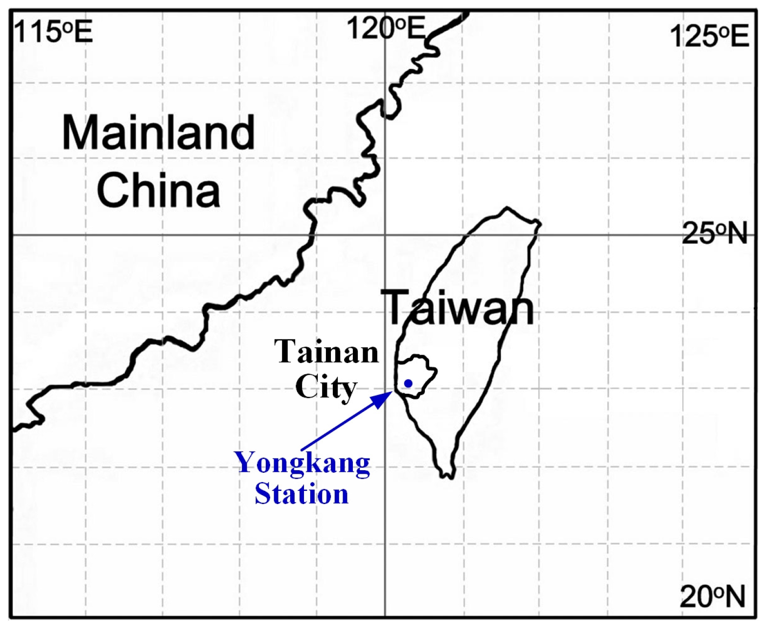
2. Study Site and Data
2.1. Ground Weather Data Set {A}
2.2. Satellite Remote-Sensing Data Set {B}
2.3. Sun Position Data Set {C}
2.3.1. Declination Angle
2.3.2. Hour Angle
2.3.3. Zenith Angle
2.3.4. Elevation Angle
2.3.5. Azimuth Angle
3. Methodology and Models
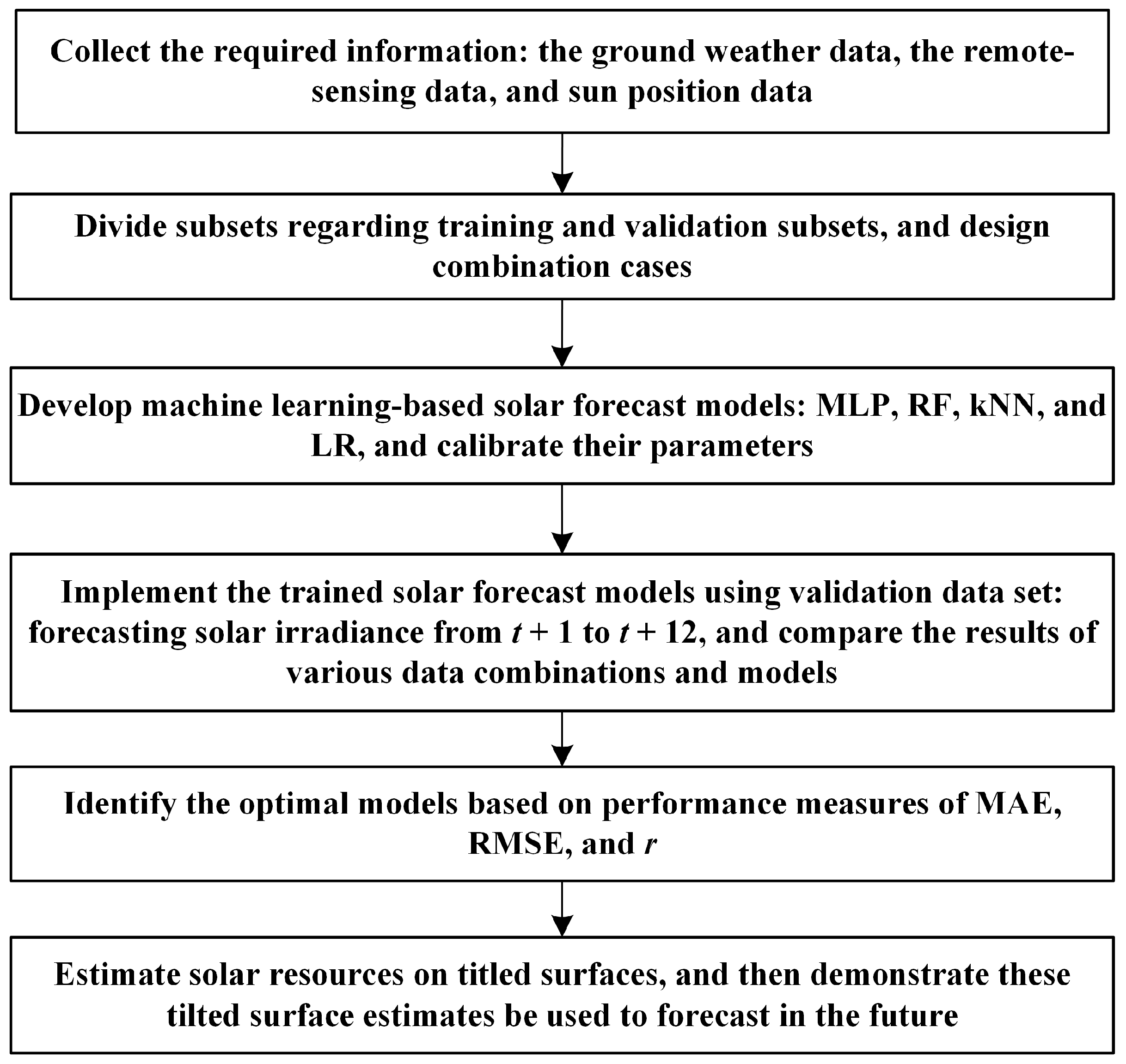
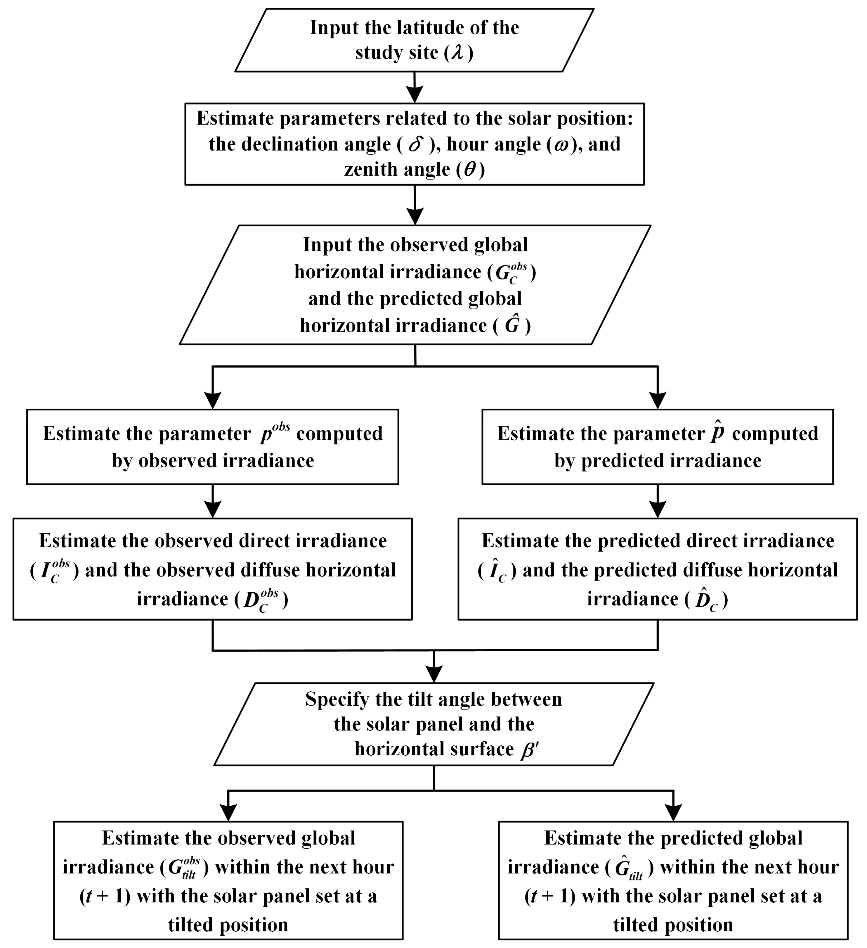
3.1. Procedures of the Methodology
3.2. Machine Learning
3.2.1. Multilayer Perceptron Neural Networks
3.2.2. Random Forests
- Step 1:
- Determine the number of decision trees required to construct RFs.
- Step 2:
- Use bootstrapping to generate new training data in existing ones. Both new and existing training data are equivalent in volume.
- Step 3:
- Use the data derived through bootstrapping to generate classification and regression trees. If the number of independent variables is P during the generation of the trees, then branching is performed on randomly selected nodes whose number of independent variables is lower than .
- Step 4:
- Repeat Steps 2 and 3 until the number of decision trees as determined in Step 1 is reached.
- Step 5:
- Analyses are performed using all decision trees. If the dependent variables are categorical, and the variable that appears the most frequently in the decision trees is deemed to be the output. If dependent variables are continuous, then the average of the prediction results from all the trees is used as the output.
3.2.3. k-Nearest Neighbor
4. Experiments and Modeling
4.1. Data Partition and Combination Cases
- Dataset combination 1: ground weather dataset, denoted by {A}.
- Dataset combination 2: ground weather dataset and satellite remote-sensing dataset ({A,B}).
- Dataset combination 3: ground weather dataset and solar position dataset ({A,C}).
- Dataset combination 4: ground weather dataset, satellite remote-sensing dataset, and solar position dataset ({A,B,C}).
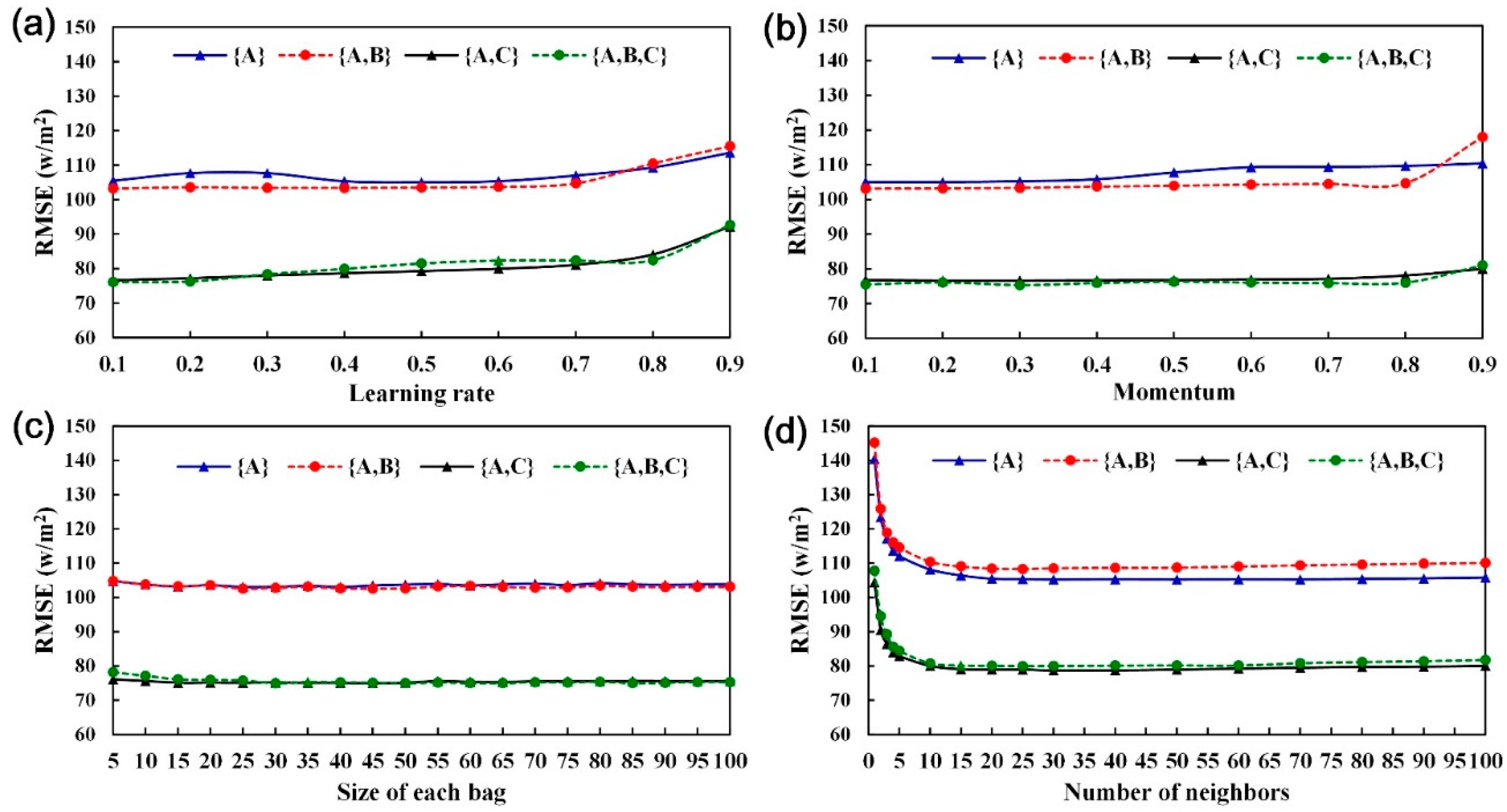
4.2. Model Parameter Setup and Calibration
4.3. Forecasting Solar Irradiance in t + 1 through the Four Dataset Combinations
4.3.1. Results of Dataset Combinations
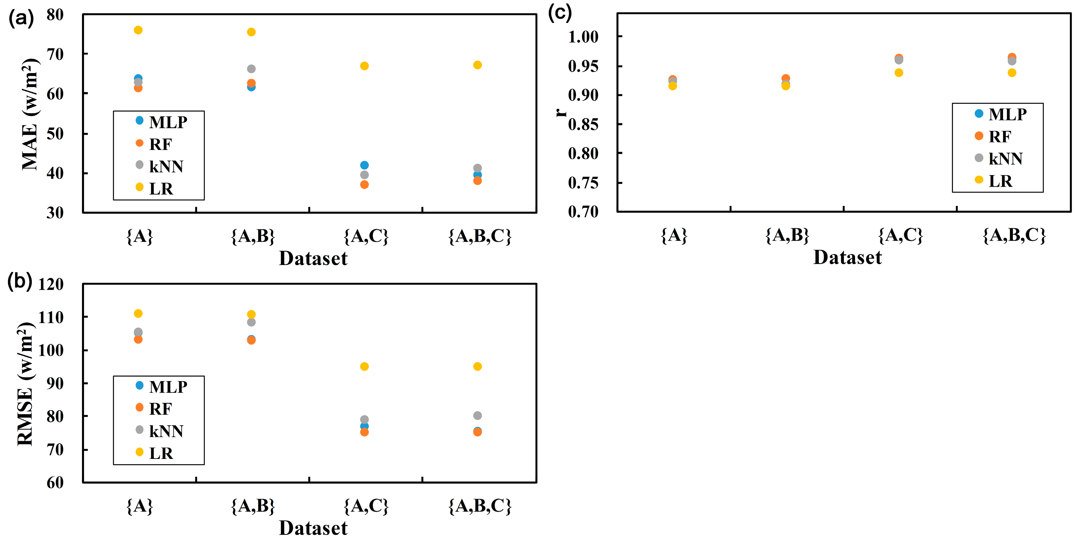
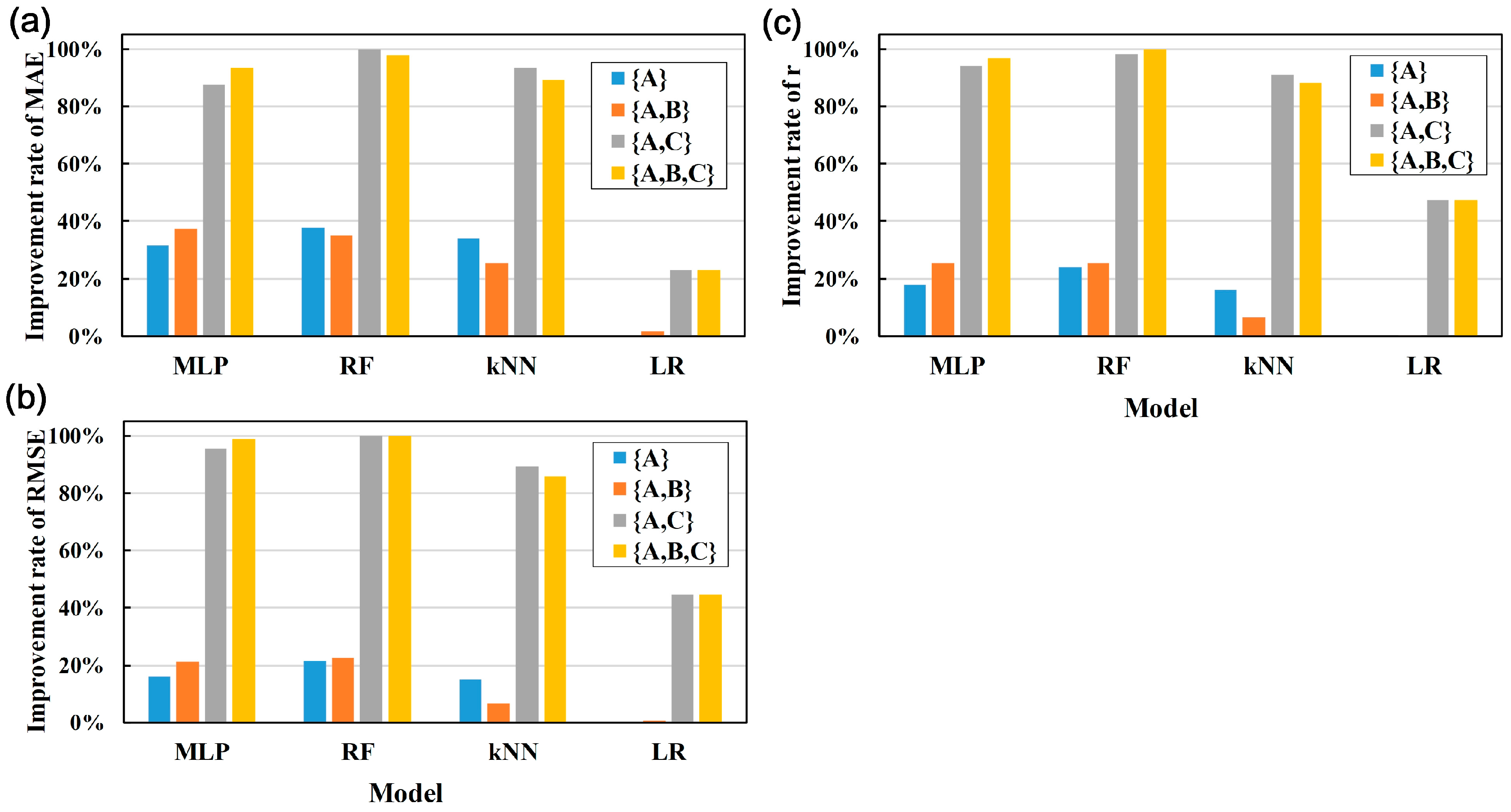
4.3.2. Evaluation
- Regarding (Figure 6a), the improvement rate was the highest in RF (100%), followed by kNN (93.6%), MLP (87.7%), and LR (23.1%).
- Regarding (Figure 6b), the improvement rate was the highest in RF (99.9%), followed by MLP (95.4%), kNN (89.4%), and LR (44.6%).
- Regarding (Figure 6c), the improvement rate was the highest in RF (98.4%), followed by MLP (94.3%), kNN (91%), and LR (47.3%).
4.4. Forecasting Solar Irradiance across Different Forecast Horizons
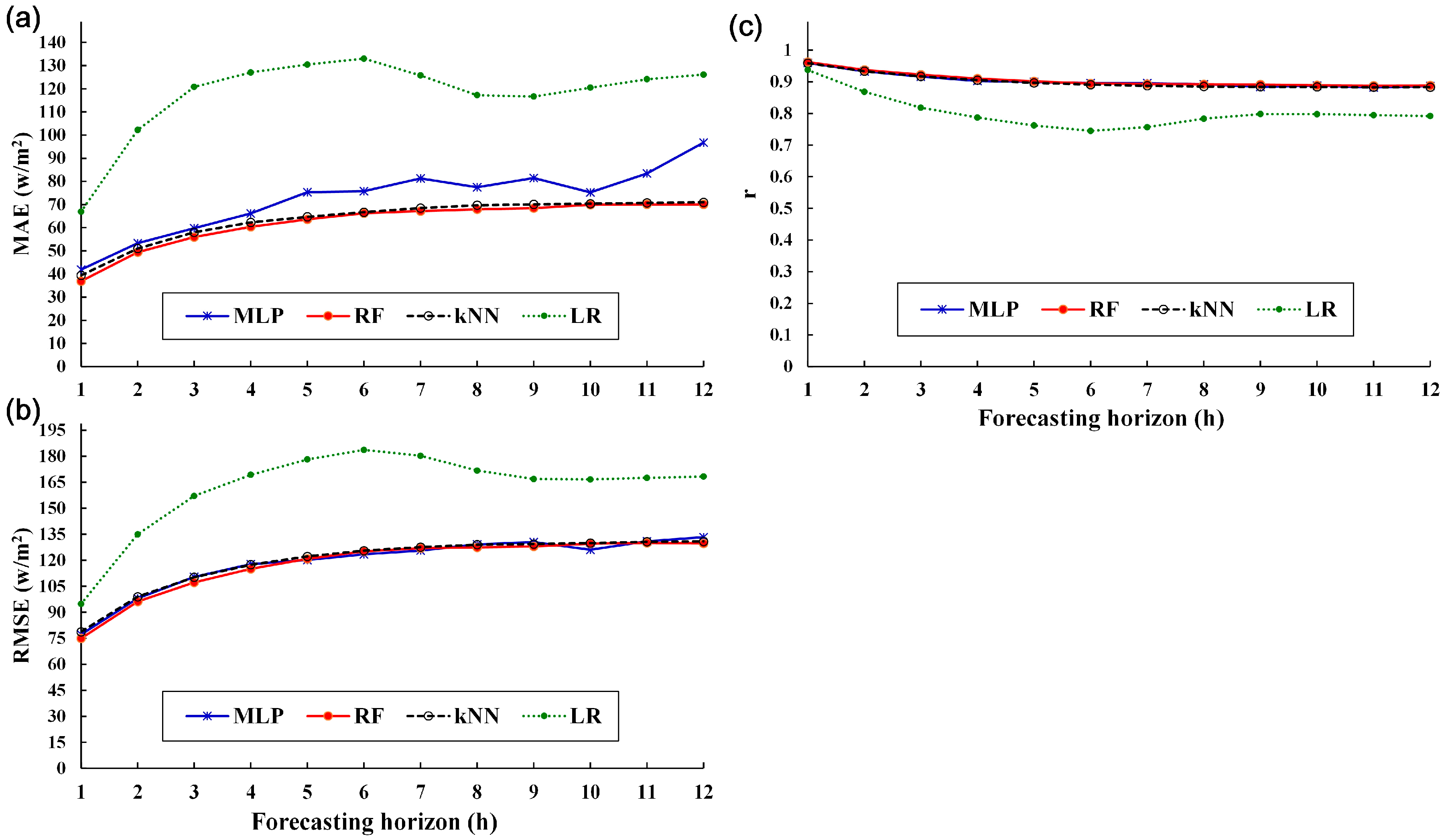
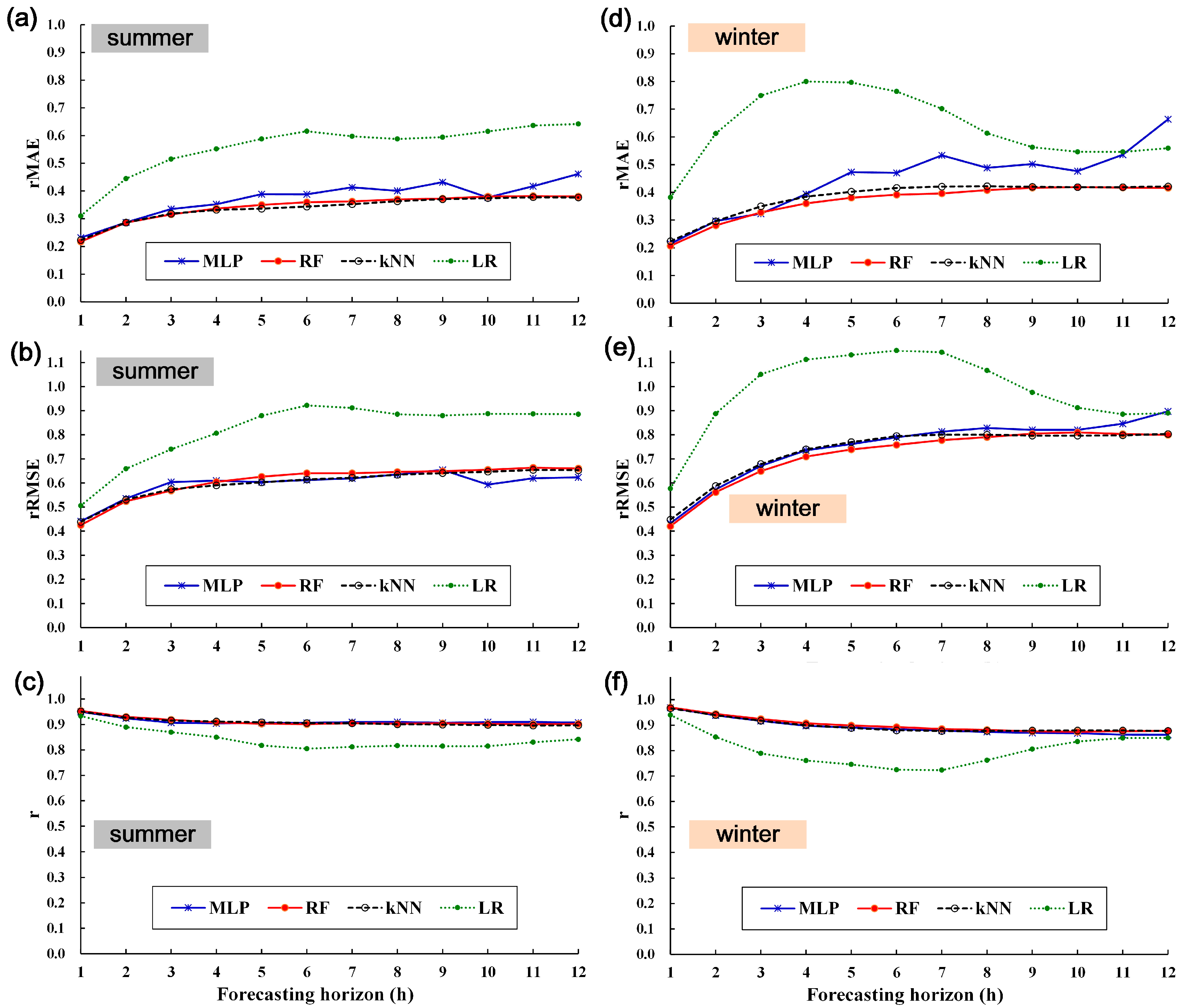
4.4.1. Prediction Results as Represented by MAE, RMSE, and r
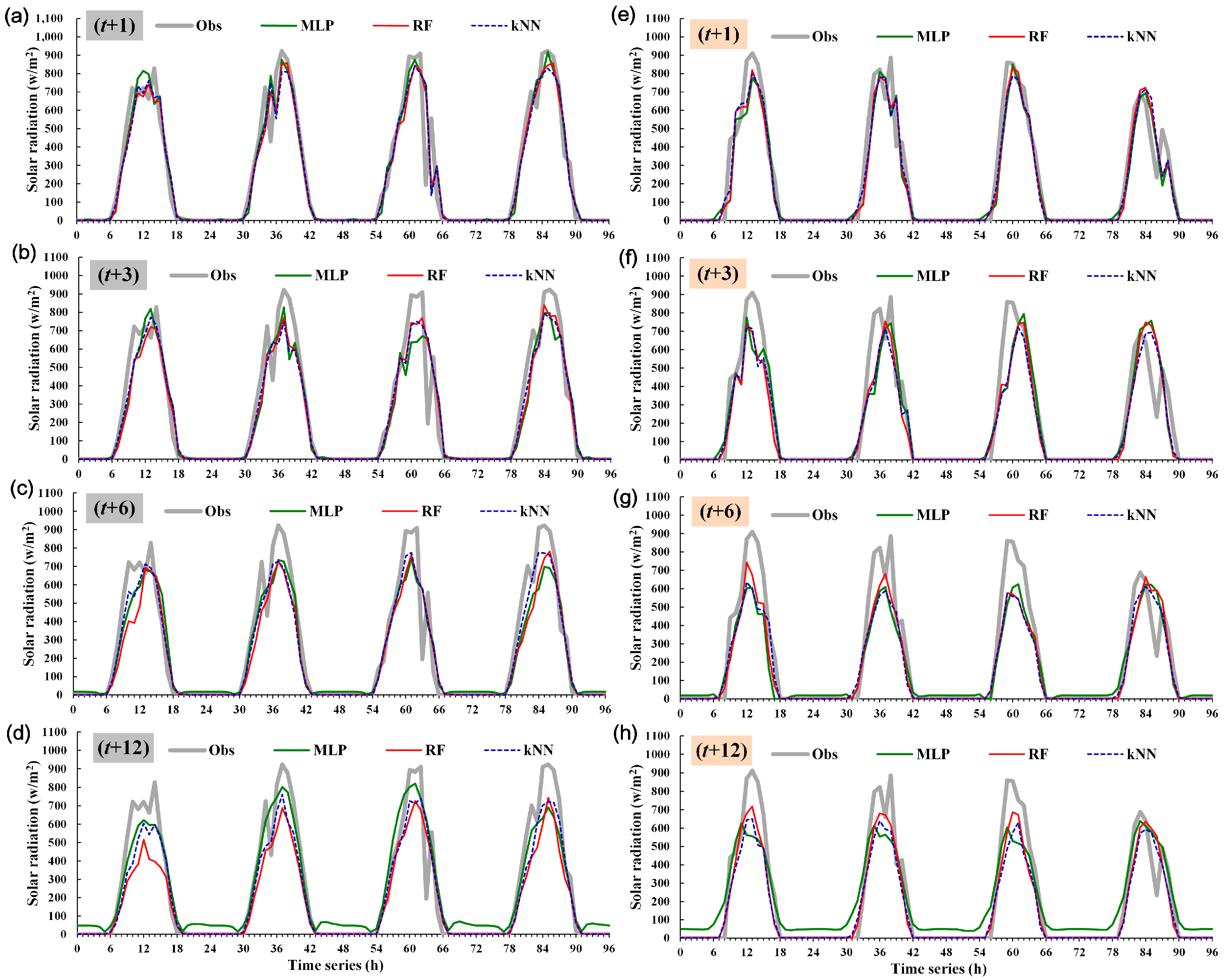
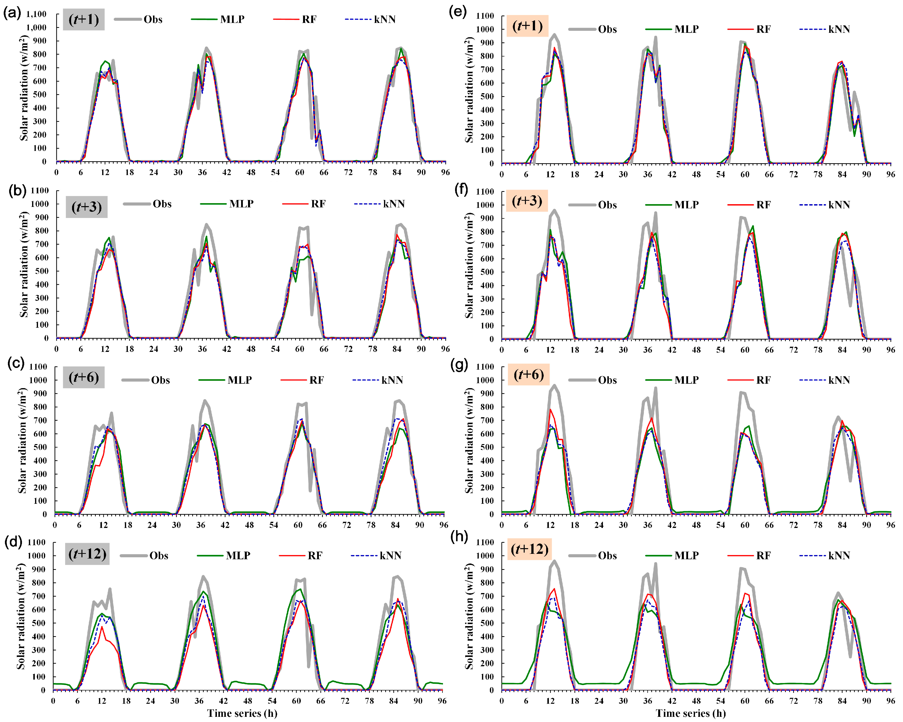
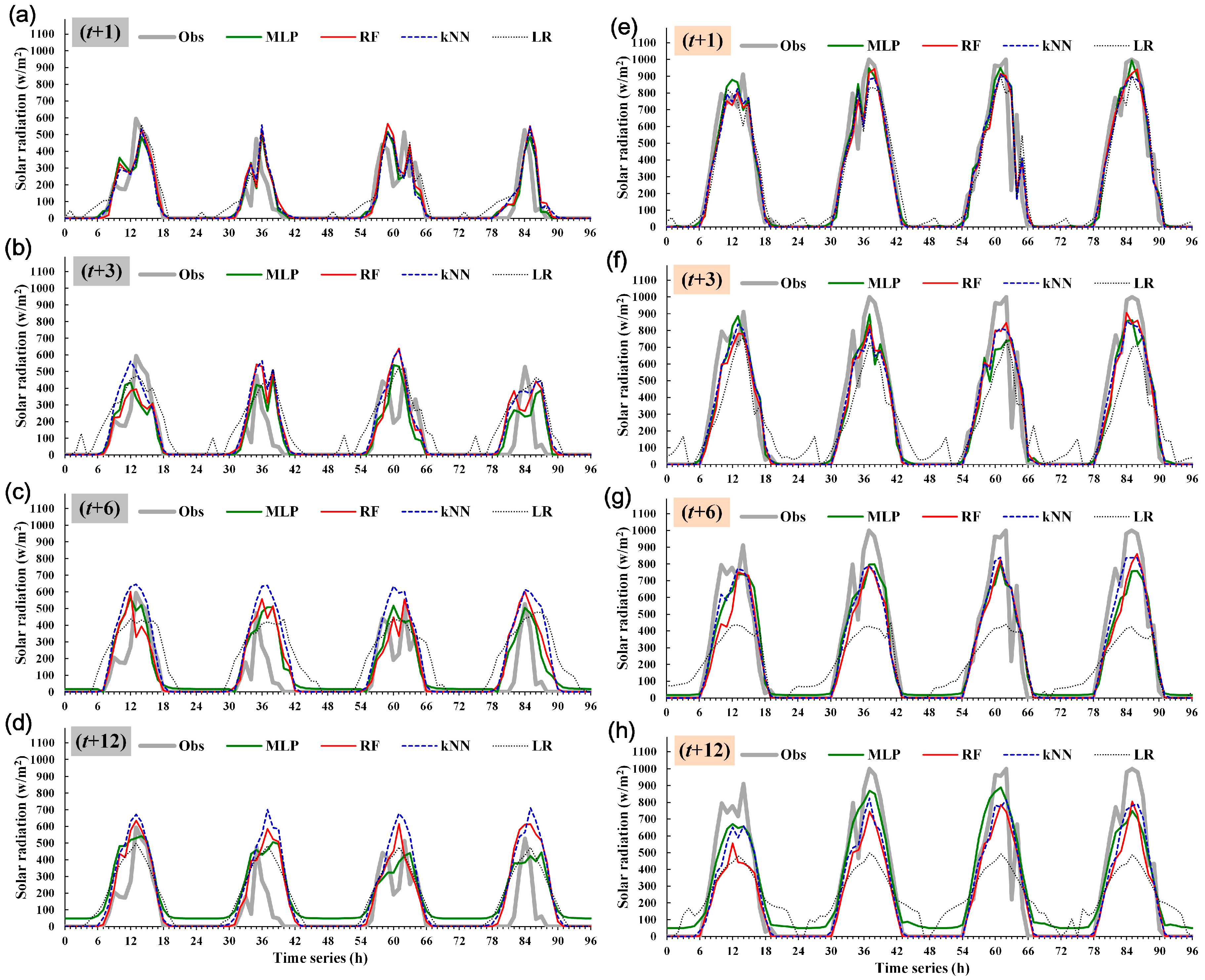
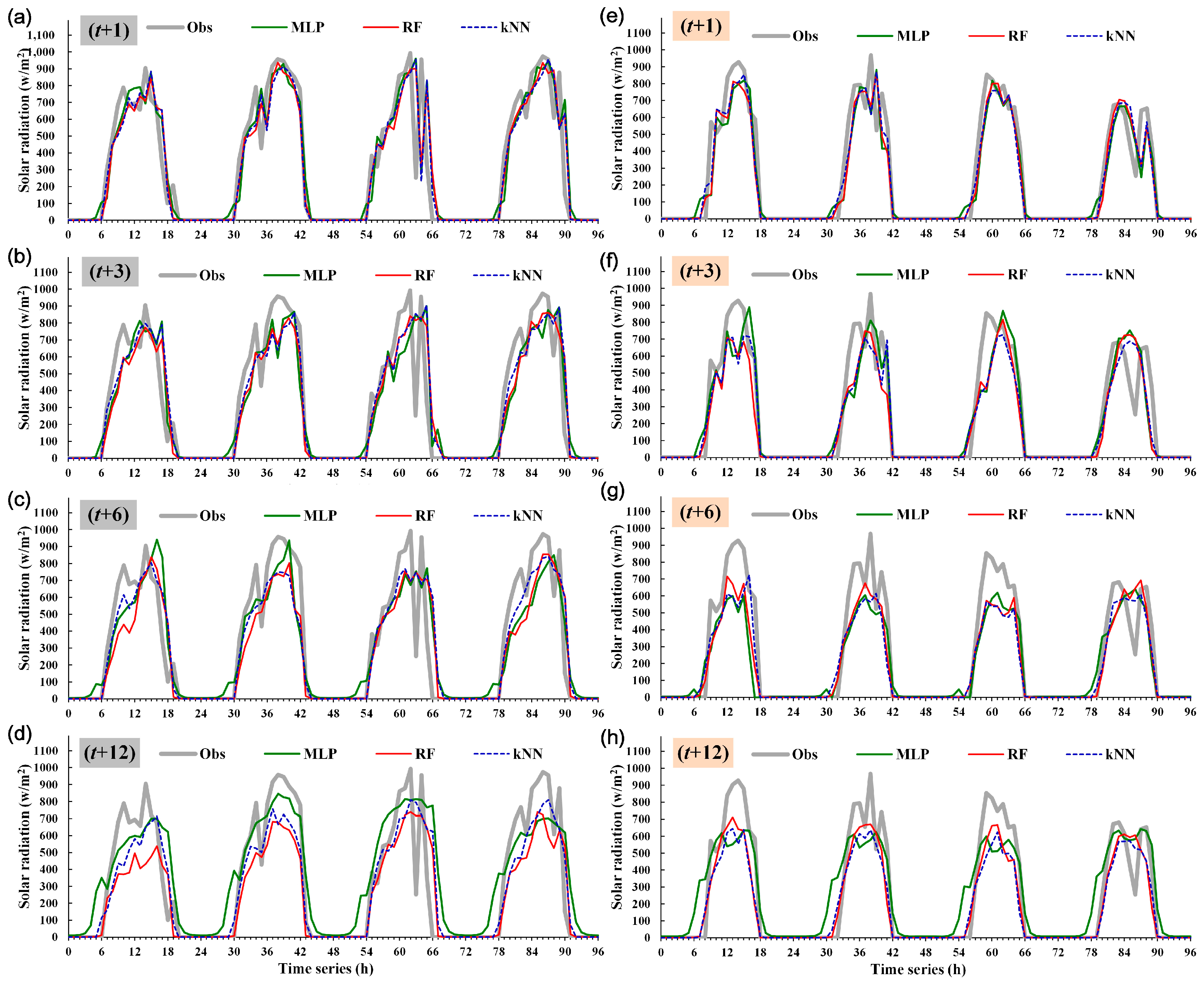
4.4.2. Predicted vs. Observed Changes in Solar Irradiance
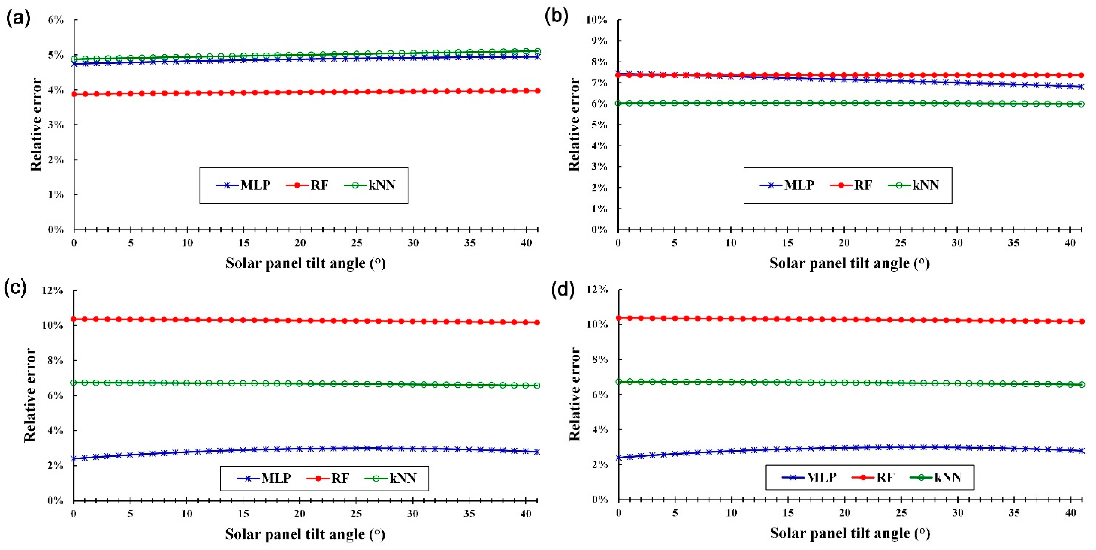
4.4.3. Prediction Errors across Seasons
5. Deriving Equations for Solar Irradiance Received by a Tilted Solar Panel
5.1. Estimating Theoretical Clear-Sky Solar Irradiance
5.1.1. Theoretical Values of GC, IC, and DC
5.1.2. Solar Incident Angle (Θ) and Global Irradiance with Tilted Solar Panels (Gtilt)
5.2. Estimating Observed and Predicted Solar Irradiance with Tilted Solar Panels
5.2.1. Estimating the Observed and Predicted Direct Irradiance and Diffuse Horizontal Irradiance
5.2.2. Estimating the Observed and Predicted Global Irradiance with the Solar Panels Set at a Tilted Position
6. Estimating Solar Irradiance with the Solar Panels Set at a Tilted Position
6.1. Estimating the Observed and Predicted Values of Global Horizontal Irradiance and Diffuse Horizontal Irradiance
6.2. Estimating the Observed and Predicted Global Irradiance with Solar Panels set at Different Tilt Angles
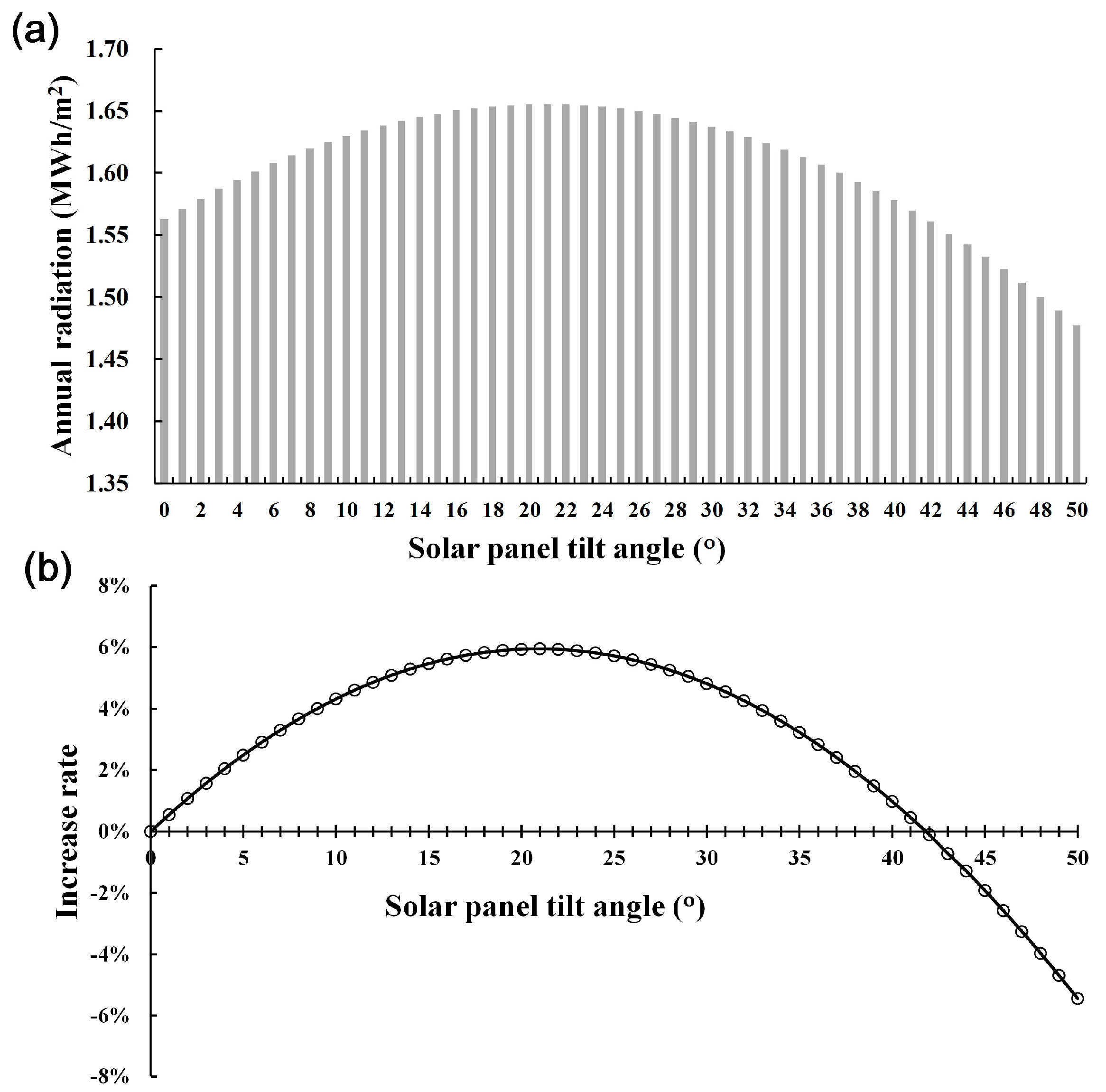
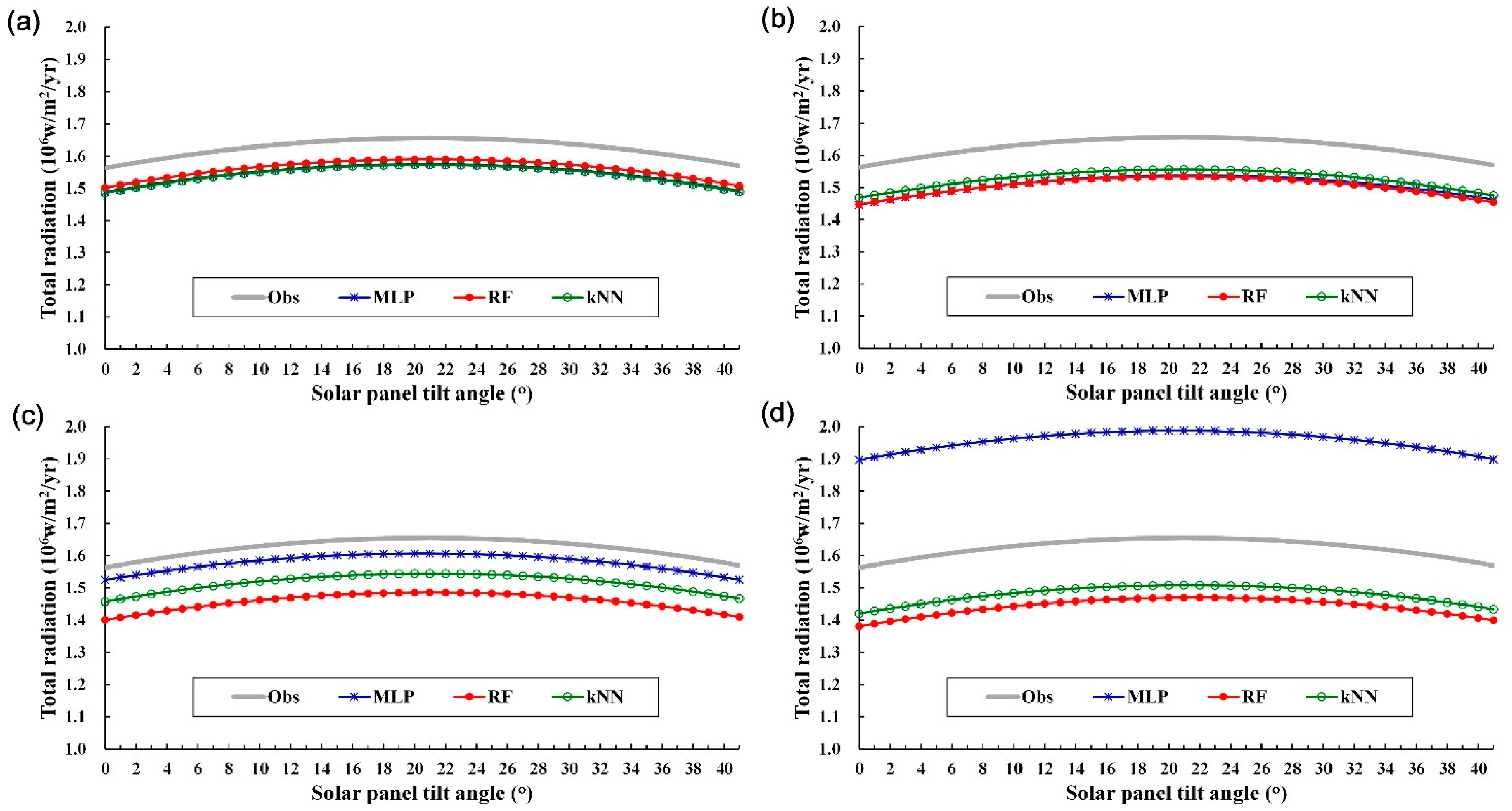
6.3. Total Annual Global Irradiance in Relation to Different Solar-Panel Tilt Angles
6.3.1. Total Annual Global Irradiance and Its Increase Rate
6.3.2. Total Annual Global Irradiance at Different Solar-panel Tilt Angles
7. Conclusions
Acknowledgments
Conflicts of Interest
References
- López, G.; Rubio, M.A.; Martı́nez, M.; Batlles, F.J. Estimation of hourly global photosynthetically active radiation using artificial neural network models. Agric. For. Meteorol. 2001, 107, 279–291. [Google Scholar] [CrossRef]
- Gomez, V.; Casanovas, A. Fuzzy modeling of solar irradiance on inclined surfaces. Sol. Energy 2003, 75, 307–315. [Google Scholar] [CrossRef]
- Reda, I.; Andreas, A. Solar position algorithm for solar radiation applications. Sol. Energy 2004, 76, 577–589. [Google Scholar] [CrossRef]
- Shen, C.; He, Y.L.; Liu, Y.W.; Tao, W.Q. Modelling and simulation of solar radiation data processing with Simulink. Simul. Model. Pract. Theory 2008, 16, 721–735. [Google Scholar] [CrossRef]
- Yeom, J.M.; Han, K.S. Improved estimation of surface solar insolation using a neural network and MTSAT-1R data. Comput. Geosci. 2010, 36, 590–597. [Google Scholar] [CrossRef]
- Chen, S.X.; Gooi, H.B.; Wang, M.Q. Solar radiation forecast based on fuzzy logic and neural networks. Renew. Energy 2013, 60, 195–201. [Google Scholar] [CrossRef]
- Inman, R.H.; Pedro, H.T.C.; Coimbra, C.F.M. Solar forecasting methods for renewable energy integration. Prog. Energy Combust. Sci. 2013, 39, 535–576. [Google Scholar] [CrossRef]
- Bode, C.A.; Limm, M.P.; Power, M.E.; Finlay, J.C. Subcanopy solar radiation model: Predicting solar radiation across a heavily vegetated landscape using LiDAR and GIS solar radiation models. Remote Sens. Environ. 2014, 154, 387–397. [Google Scholar] [CrossRef]
- Li, Z.; Rahman, S.M.; Vega, R.; Dong, B. A hierarchical approach using machine learning methods in solar photovoltaic energy production forecasting. Energies 2016, 9, 55. [Google Scholar] [CrossRef]
- Persson, C.; Bacher, P.; Shiga, T.; Madsen, H. Multi-site solar power forecasting using gradient boosted regression trees. Sol. Energy 2017, 150, 423–436. [Google Scholar] [CrossRef]
- Yousif, J.H.; Kazem, H.A.; Boland, J. Predictive models for photovoltaic electricity production in hot weather conditions. Energies 2017, 10, 971. [Google Scholar] [CrossRef]
- Platnick, S.; Valero, F.P.J. A validation of a satellite cloud retrieval during ASTEX. J. Atmos. Sci. 1995, 52, 2985–3001. [Google Scholar] [CrossRef]
- Stephens, G. Cloud feedbacks in the climate system: A critical review. J. Clim. 2005, 18, 237–273. [Google Scholar] [CrossRef]
- Kühnlein, M.; Appelhans, T.; Thies, B.; Kokhanovsky, A.A.; Nauss, T. An evaluation of a semi-analytical cloud property retrieval using MSG SEVIRI, MODIS and CloudSat. Atmos. Res. 2013, 122, 111–135. [Google Scholar] [CrossRef]
- Brandau, C.L.; Russchenberg, H.W.J.; Knap, W.H. Evaluation of ground-based remotely sensed liquid water cloud properties using shortwave radiation measurements. Atmos. Res. 2010, 96, 366–377. [Google Scholar] [CrossRef]
- Journée, M.; Muller, R.; Bertrand, C. Solar resource assessment in the Benelux by merging Meteosat-derived climate data and ground measurements. Sol. Energy 2012, 86, 3561–3574. [Google Scholar] [CrossRef]
- Nauss, T.; Kokhanovsky, A.A. Retrieval of warm cloud optical properties using simple approximations. Remote Sens. Environ. 2011, 115, 1317–1325. [Google Scholar] [CrossRef]
- Wong, M.S.; Zhu, R.; Liu, Z.; Lu, L.; Chan, W.K. Estimation of Hong Kong’s solar energy potential using GIS and remote sensing technologies. Renew. Energy 2016, 99, 325–335. [Google Scholar] [CrossRef]
- Shafiullah, G.M. Hybrid renewable energy integration (HREI) system for subtropical climate in Central Queensland, Australia. Renew. Energy 2016, 96 Pt A, 1034–1053. [Google Scholar] [CrossRef]
- Lin, C.; Wei, C.C.; Tsai, C.C. Prediction of influential operational compost parameters for monitoring composting process. Environ. Eng. Sci. 2016, 33, 494–506. [Google Scholar] [CrossRef]
- Breiman, L. Random forests. Mach. Learn. 2001, 45, 5–32. [Google Scholar] [CrossRef]
- Kühnlein, M.; Appelhans, T.; Thies, B.; Nauß, T. Precipitation estimates from MSG SEVIRI daytime, nighttime, and twilight data with random forests. J. Appl. Meteorol. Climatol. 2014, 53, 2457–2480. [Google Scholar] [CrossRef]
- Duda, R.O.; Hart, P.E.; Stork, D.G. Pattern Classification, 2nd ed.; John Wiley & Sons Ltd.: Hoboken, NJ, USA, 2000. [Google Scholar]
- Toussaint, G.T. Geometric proximity graphs for improving nearest neighbor methods in instance-based learning and data mining. Int. J. Comput. Geom. Appl. 2005, 15, 101–150. [Google Scholar] [CrossRef]
- Wei, C.C. Comparing lazy and eager learning models for water level forecasting in river-reservoir basins of inundation regions. Environ. Model. Softw. 2015, 63, 137–155. [Google Scholar] [CrossRef]
- Savtchenko, A.; Ouzounov, D.; Ahmad, S.; Acker, J.; Leptoukh, G.; Koziana, J.; Nickless, D. Terra and Aqua MODIS products available from NASA GES DAAC. Adv. Space Res. 2004, 34, 710–714. [Google Scholar] [CrossRef]
- Chen, F.C. A Meteorology Assessment for Photovoltaic Generation. Master’s Thesis, Southern Taiwan University of Science and Technology, Tainan, Taiwan, 2006. (In Chinese). [Google Scholar]
- Exell, R.H.B. A mathematical model for solar radiation in South-East Asia (Thailand). Sol. Energy 1981, 26, 161–168. [Google Scholar] [CrossRef]
- Markvart, T. Solar Electricity; John Wiley & Sons Ltd.: New York, NY, USA, 1994. [Google Scholar]
- Wei, C.C.; Hsu, N.S. Multireservoir flood-control optimization with neural-based linear channel level routing under tidal effects. Water Resour. Manag. 2008, 22, 1625–1647. [Google Scholar] [CrossRef]
- Ho, T.K. Random Decision Forest. In Proceedings of the 3rd International Conference on Document Analysis and Recognition, Montreal, QC, Canada, 14–18 August 1995. [Google Scholar]
- Ho, T.K. The random subspace method for constructing decision forests. IEEE Trans. Pattern Anal. Mach. Intell. 1998, 20, 832–844. [Google Scholar]
- Chen, S.Z. Evaluating the Effectiveness of Random Forest Model. Master’s Thesis, National Chiao Tung University, Hsinchu City, Taiwan, 2014. (In Chinese). [Google Scholar]
- Trenn, S. Multilayer perceptrons: Approximation order and necessary number of hidden units. IEEE Trans. Neural Netw. 2008, 19, 836–844. [Google Scholar] [CrossRef] [PubMed]


| Data Set | Attribute | Unit | Min–Max | Mean | Standard Deviation |
|---|---|---|---|---|---|
| Ground weather | Atmospheric pressure | hPa | 973.8–1031.5 | 1011.2 | 5.72 |
| Wind speed | m/s | 0–18.4 | 2.83 | 1.70 | |
| Precipitation | mm | 0–95 | 0.23 | 1.91 | |
| Temperature | °C | 5.6–35.9 | 24.3 | 5.38 | |
| Relative humidity | % | 23–100 | 74.0 | 10.17 | |
| Radiation | w/m2 | 0–1125.00 | 162.04 | 249.38 | |
| Satellite Remote-sensing | Aerosol optical depth | - | 0.18–10.74 | 2.80 | 1.56 |
| Water vapor | cm | 0.15–77.21 | 37.47 | 13.72 | |
| Cirrus reflectance | - | 0.25–67.42 | 2.92 | 4.99 | |
| Cloud fraction | - | 0.93–100 | 68.50 | 28.76 | |
| Sun Position | Declination angle | Deg. | −23.45–23.45 | −0.01 | 16.58 |
| Hour angle | Deg. | −165.00–80.00 | 7.50 | 103.83 | |
| Zenith angle | Deg. | 0.01–179.99 | 90.00 | 43.83 | |
| Elevation angle | Deg. | −89.99–89.99 | 0.00 | 43.83 | |
| Azimuth angle | Deg. | −90.00–90.00 | 0.00 | 65.09 |
| Model Case | MLP | RF | kNN | |
|---|---|---|---|---|
| Learning Rate | Momentum | Size of Each Bag | Number of Neighbors | |
| Dataset {A} | 0.5 | 0.2 | 40 | 30 |
| Dataset {A, B} | 0.1 | 0.1 | 25 | 25 |
| Dataset {A, C} | 0.1 | 0.2 | 45 | 30 |
| Dataset {A, B, C} | 0.1 | 0.3 | 30 | 25 |
| Performance | Case {A} | Case {A,B} | Case {A,C} | Case {A,B,C} |
|---|---|---|---|---|
| MAE | 62.52 | 63.23 | 39.33 | 39.42 |
| RMSE | 104.45 | 104.67 | 76.78 | 76.75 |
| r | 0.924 | 0.923 | 0.960 | 0.961 |
| Season | Performance | t + 1 | t + 6 | ||||||
|---|---|---|---|---|---|---|---|---|---|
| MLP | RF | kNN | LR | MLP | RF | kNN | LR | ||
| Spring | MAE (w/m2) | 39.4 | 37.4 | 41.1 | 57.9 | 76.0 | 68.5 | 70.6 | 123.1 |
| rMAE | 0.209 | 0.198 | 0.218 | 0.307 | 0.403 | 0.363 | 0.374 | 0.652 | |
| RMSE (w/m2) | 74.6 | 73.8 | 80.0 | 89.0 | 125.6 | 129.7 | 135.2 | 184.5 | |
| rRMSE | 0.395 | 0.391 | 0.424 | 0.472 | 0.665 | 0.687 | 0.716 | 0.978 | |
| r | 0.964 | 0.965 | 0.959 | 0.950 | 0.896 | 0.888 | 0.876 | 0.767 | |
| Summer | MAE (w/m2) | 50.7 | 47.6 | 48.8 | 67.8 | 84.9 | 78.7 | 75.2 | 134.7 |
| rMAE | 0.232 | 0.217 | 0.223 | 0.310 | 0.388 | 0.360 | 0.344 | 0.616 | |
| RMSE (w/m2) | 96.5 | 93.1 | 95.9 | 110.6 | 134.0 | 140.1 | 134.4 | 201.6 | |
| rRMSE | 0.441 | 0.426 | 0.438 | 0.506 | 0.613 | 0.640 | 0.614 | 0.922 | |
| r | 0.950 | 0.954 | 0.951 | 0.933 | 0.906 | 0.901 | 0.906 | 0.805 | |
| Autumn | MAE (w/m2) | 36.2 | 34.1 | 36.8 | 56.0 | 72.4 | 63.7 | 63.8 | 107.6 |
| rMAE | 0.218 | 0.205 | 0.222 | 0.338 | 0.436 | 0.384 | 0.384 | 0.648 | |
| RMSE (w/m2) | 72.1 | 70.8 | 73.4 | 89.3 | 122.2 | 123.7 | 121.3 | 170.1 | |
| rRMSE | 0.434 | 0.426 | 0.442 | 0.538 | 0.736 | 0.745 | 0.731 | 1.025 | |
| r | 0.962 | 0.964 | 0.962 | 0.941 | 0.892 | 0.892 | 0.892 | 0.781 | |
| Winter | MAE (w/m2) | 29.4 | 28.5 | 30.7 | 52.4 | 64.6 | 53.8 | 57.1 | 104.9 |
| rMAE | 0.214 | 0.207 | 0.223 | 0.382 | 0.470 | 0.392 | 0.416 | 0.764 | |
| RMSE (w/m2) | 59.4 | 57.8 | 61.5 | 79.2 | 108.4 | 104.1 | 109.1 | 157.9 | |
| rRMSE | 0.432 | 0.421 | 0.448 | 0.577 | 0.790 | 0.758 | 0.795 | 1.150 | |
| r | 0.968 | 0.969 | 0.966 | 0.940 | 0.884 | 0.893 | 0.880 | 0.725 | |
© 2017 by the author. Licensee MDPI, Basel, Switzerland. This article is an open access article distributed under the terms and conditions of the Creative Commons Attribution (CC BY) license (http://creativecommons.org/licenses/by/4.0/).
Share and Cite
Wei, C.-C. Predictions of Surface Solar Radiation on Tilted Solar Panels using Machine Learning Models: A Case Study of Tainan City, Taiwan. Energies 2017, 10, 1660. https://doi.org/10.3390/en10101660
Wei C-C. Predictions of Surface Solar Radiation on Tilted Solar Panels using Machine Learning Models: A Case Study of Tainan City, Taiwan. Energies. 2017; 10(10):1660. https://doi.org/10.3390/en10101660
Chicago/Turabian StyleWei, Chih-Chiang. 2017. "Predictions of Surface Solar Radiation on Tilted Solar Panels using Machine Learning Models: A Case Study of Tainan City, Taiwan" Energies 10, no. 10: 1660. https://doi.org/10.3390/en10101660