1. Introduction
Nowadays, many efforts have been devoted to revealing the hidden patterns in fault-related signals. Different possible signal sources, such as vibration signal and acoustic signal, are investigated to provide more accurate and efficient methods [
1,
2,
3]. Although vibration signal is adopted in most fault diagnosis cases, acoustic signal is more desirable in some implementations due to its unique merits [
2]. The first advantage for acoustic signal is the low hardware cost because of its independence of direction. Only one acoustic sensor is required to achieve the same functionality as that of vibration signal. Second, when compared with vibration signal, acoustic signal is relatively immune to the underlying structural resonances. Third, it is easier for acoustic sensor to capture incipient fault information than the vibration sensor as it is more sensitive [
4]. These advantages, in two aspects, fulfill the functional requirements of fault diagnosis. On the one hand, incipient faults would likely generate weak vibration energy, which could hardly cause any significant physical degradation within the solid structure, which makes it impossible for the vibration sensor to capture any useful pattern. On the other hand, acoustic sensor can cover a much more extensive range of frequencies which enables it to be embedded with much more extended types of fault signals [
5,
6]. However, the disadvantages accompanying the merits are the low signal to noise ratio (SNR) and low computational efficiency. To solve this problem, proposing a suitable signal processing approach for acoustic signal is essential.
To handle different implementation situations, many methods have been developed like fast Fourier transform (FFT) [
7], wavelet transform [
8], and empirical mode decomposition (EMD) [
9,
10]. FFT could generate the statistical average characteristics under the circumstance of steady operations, but it cannot deal with time and frequency domain problems. The wavelet transform, as a time-frequency analysis approach, is widely used in fault feature extraction [
11], but it could only use certain frequency bands to deal with the acquired signal [
12].
EMD is a method proposed recently for analyzing nonlinear and non-stationary signals. The main idea is to use the envelope lines and the mean value of a signal to decompose it into several intrinsic mode functions (IMFs) [
13], and by analyzing each of the obtained IMFs, the patterns hiding in the original signal could be accurately and effectively extracted. Although the investigations into EMD have been reported in the literature in the field of fault diagnosis [
14], the major disadvantages are the mode mixing issues and redundant IMFs, which degrades the performance of EMD in application. To solve the problems of mode mixing and redundant IMFs, the traditional EMD has been modified, namely ensemble empirical mode decomposition (EEMD) [
15], to fix the mode mixing problem [
16], and correlation coefficient technology is applied to eliminate the redundant IMFs. The detailed explanation will be introduced in
Section 3.2.
Although the proposed EEMD helps to alleviate the problem of mode mixing, it still has to face the problem of the large dataset because fundamentally it decomposes one signal into ten or more IMFs. In general, the large size dataset could compromise the performance of the classifiers. To improve the overall performance, useful information should be further extracted during signal processing to make the decomposed IMFs more meaningful and more representative.
As the generated IMFs could perfectly form a matrix, singular value decomposition (SVD) becomes one of the suitable solutions because it could reduce the size of a matrix and reveal the hidden information in it [
17]. As the singular value of a matrix is relatively stable and it could represent its natural characteristic, it is desirable to be used to detect periodic faults. Moreover, it is not necessary to manually choose the reconstruction parameters in SVD because the initial feature vector matrix can be generated by combining the IMFs directly [
18]. When considering the periodic impulse could reveal related faults by singular values of the matrixes while applying SVD, the SVD technique based on EEMD is proposed. To further solve the high computational cost problem, sample entropy (SampEn) as a feature selection method can be employed to reduce the input size and dimension for the fault classifiers [
19], as it could also select the fault features from irregular faults of each IMF generated by EMD method [
20]. As the faults of rotating machinery can usually be classified into two types as periodic and irregular faults, this study proposed a proper feature selection method via the combination of SVD and SampEn to generate a feature matrix that could identify both irregular and periodic faults adequately.
Conventional pattern recognition methods always generate binary results, which could not meet the demand of modern implementations. As a result, probabilistic neural network (PNN) and relevance vector machine (RVM) [
21,
22] are proposed to serve as probabilistic classifiers. The prevalence of PNN is hindered by its complexity and the input-related training time. For RVM, a Bayesian based support vector machine, as it needs to deal with Hessian matrix, which computes attains
O(
N2), it can not handle big data problems. Recently, a sparse Bayesian based extreme learning machine (SBELM) emerged as a more advanced classifier [
23]. The Sparse Bayesian framework is adopted to modify the probabilistic classifier extreme learning machine (ELM) to reduce the training time and entitle it with the ability to effectively handle big data problems. To make the proposed approach more practical, a pairwise coupling strategy, named one versus one strategy (1vs1), is further incorporated, thus making it possible to deal with multi-classification problems [
24]. The new classifier is named pairwise-coupled sparse Bayesian extreme learning machine (PC-SBELM). The main advantage of the pairwise coupling strategy is to include the correlation between different faults that make the probabilistic estimation more accurate. The details of how the proposed 1vs1 strategy works will be discussed in
Section 2.2. Although a similar framework is proposed by the authors in [
25], the new framework here adopts a more effective technique, correlation coefficient, to select the suitable number of IMF to reduce the redundant information and improve the SNR. Moreover, the number of periodic and irregular faults tested in the experiments is extended from four to six. Besides, to verify the effectiveness of the proposed classifier, pairwise-coupled relevance vector machine (PC-RVM) and pairwise-coupled probabilistic neural network (PC-PNN) are also adopted as comparisons.
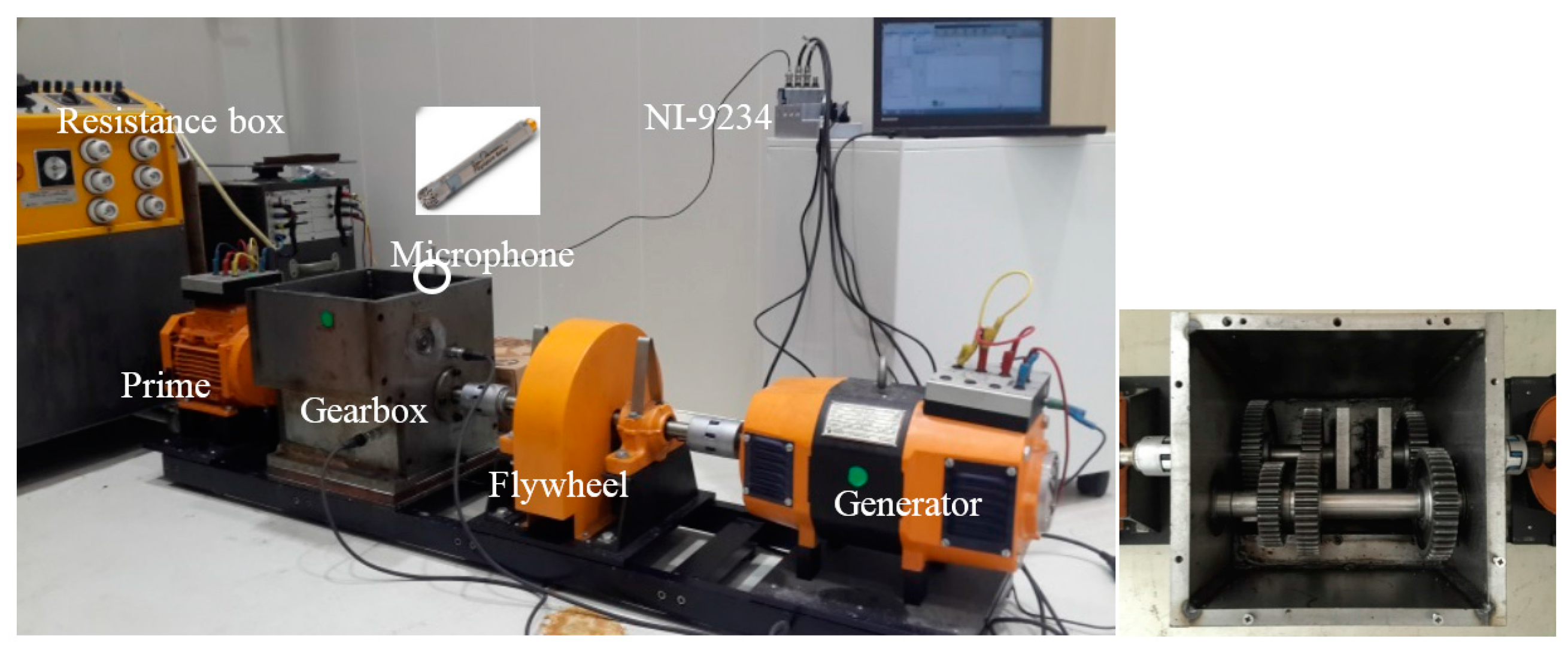
The organization of this paper is as follows. The second section introduces the proposed framework and the methods adopted. Then, a test rig is set up and the corresponding signal pre-processing is discussed in
Section 3. In the fourth section, experimental results are generated and compared with the aforesaid existing approaches. The last section summarizes the proposed system and conclusions are given.
2. Proposed Frameworks
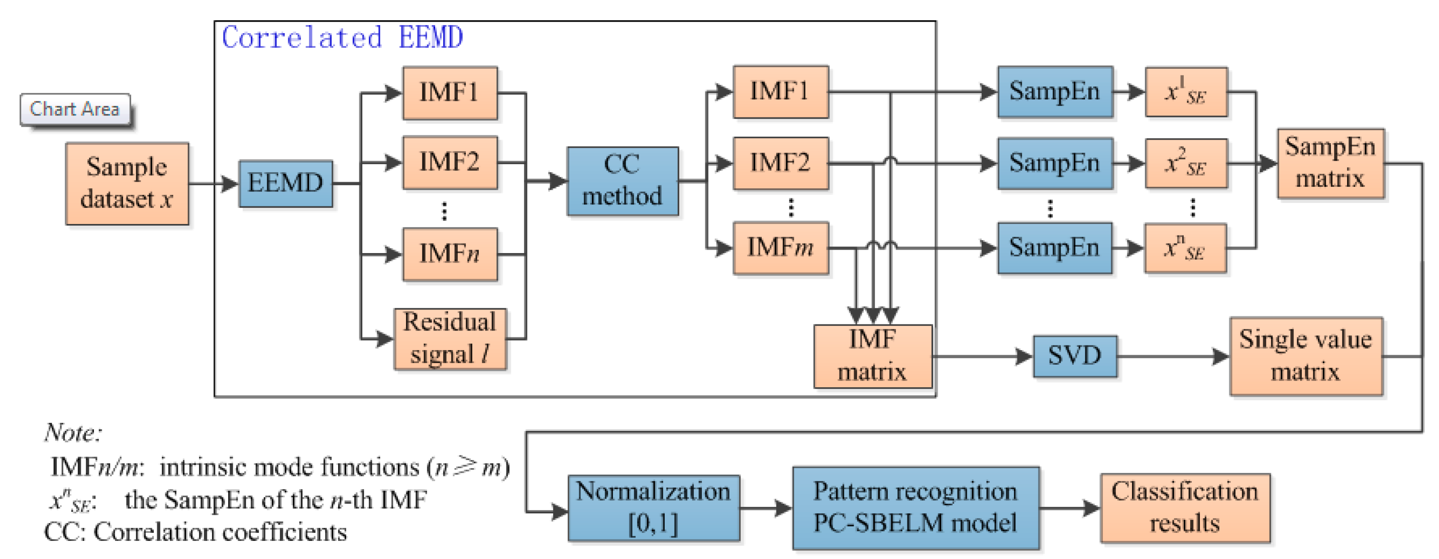
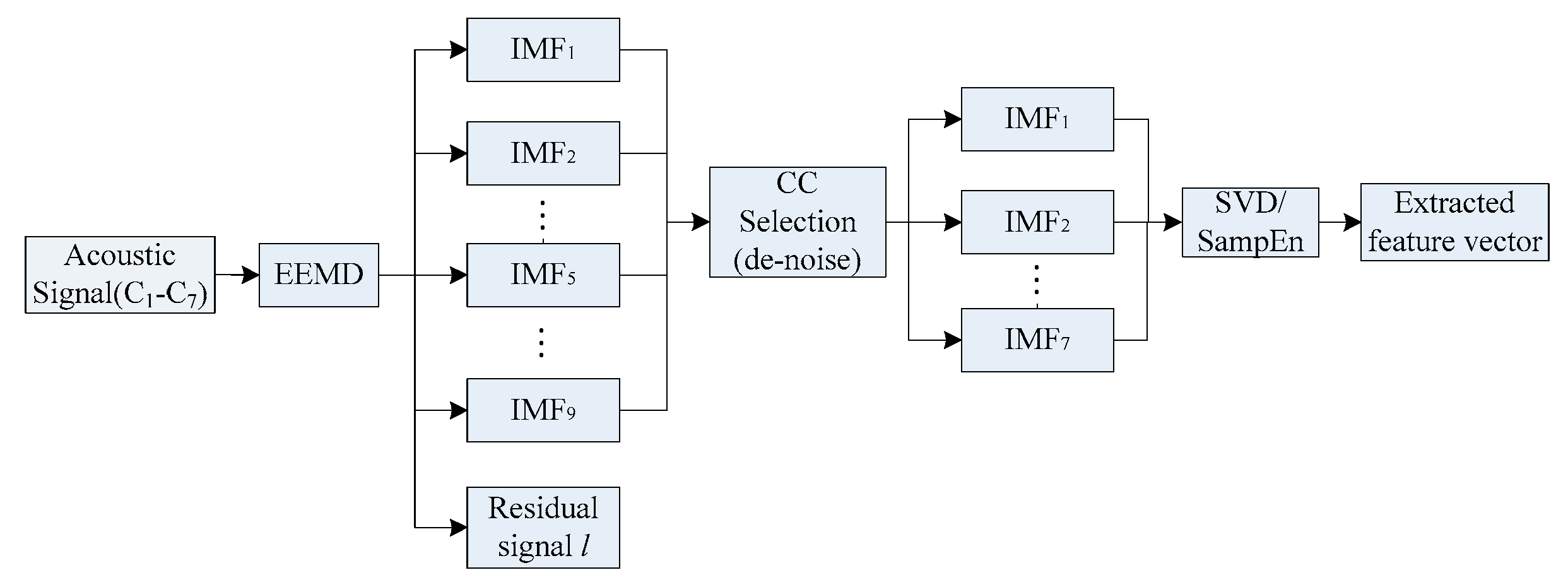
Figure 1 shows the proposed periodic and irregular fault diagnosis system for rotating machinery. The proposed fault diagnosis system consists of two components, namely, (1) data processing and (2) pattern recognition, which will be thoroughly discussed in the following sub-sections.
In the phase of data processing, EEMD decomposes the acquired acoustic signal into a series of IMFs. To de-noise by reducing the redundant IMFs, correlation coefficient method is applied to select the useful IMFs. After the signal being de-noised, SVD and SampEn would generate a selected feature matrix that contains both irregular and periodic fault features. Finally, the proposed pattern recognition method, PC-SBELM, will be verified using the extracted features in training, validating and testing.
2.1. Data Processing
2.1.1. Ensemble Empirical Mode Decomposition
As conventional EMD suffers from mode mixing, EEMD is adopted in this study. It employs white noises of certain amplitudes to help separate different IMFs more effectively and calculates the ensemble mean of each decomposition to eliminate the white noise. The general rule for the added white noise is that small amplitude white noise should be added to high-frequency components and large amplitude white noise for low-frequency components. In [
26], the recommended standard deviation range is from 0.1 to 0.4. The algorithm can be summarized as:
Set the ensemble number as E, the white noise (amplitude) and e = 1.
For
eth trail, a white noise with corresponding amplitude will be added to the investigated signal.
where
ne is the
eth white noise, and
xe is the resultant signal.
Then xe will be further decomposed by conventional EMD into I IMFs as ci,e(t), where I is the number of IMF and ci,e is the ith IMF of the eth trial.
Let e = e + 1 and repeat steps 2 and 3 with different white noise until n = E.
Find the ensemble mean to eliminate the white noise:
Treat the means as the final results.
After the decomposition, the dimension of the original signal increased because of the generated IMFs, but the data points in each IMF is the same as the original signal. Depending on the sampling rate, the number of points of a signal can be very large, implying that a very large input vector needs to be constructed for the fault classifiers. Moreover, it is generally believed that high dimensional and large input vector can undesirably compromise the performance of the classifier. Therefore, it is necessary to extract useful features from the pre-processed signal to reduce the data dimension and scale.
2.1.2. Correlation Coefficient Based EEMD
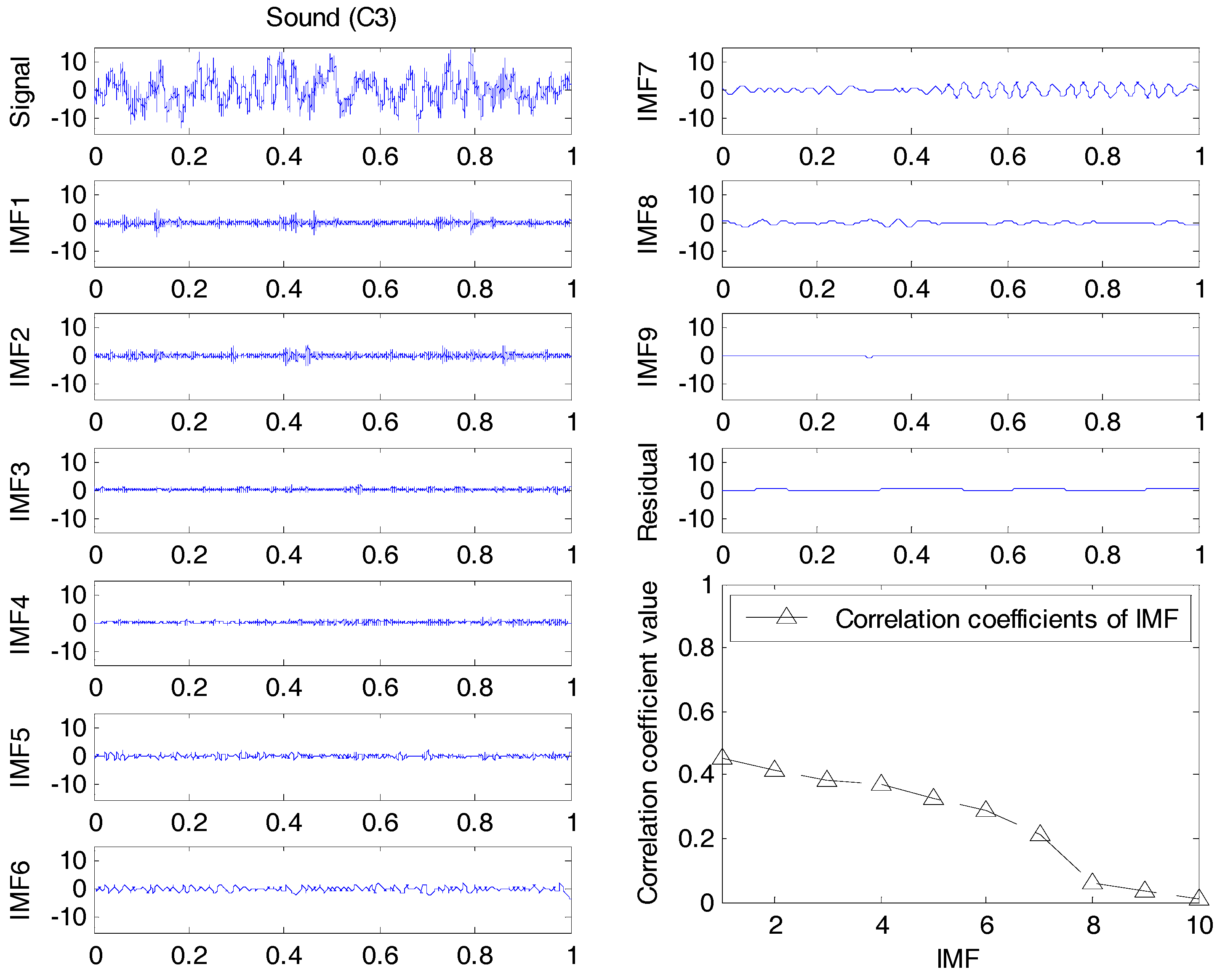
In order to reduce the number of IMFs and improve the overall computational efficiency, the correlation coefficient of an IMF
Ii(
t) to the original signal
x(
t) is calculated as:
where the overline denotes the mean value of certain variables and
M is the number of IMFs. The larger the coefficient is, the more significant fault information an IMF could contain. To improve the SNR, those IMFs with a small
value are treated as noise and are ignored. The correlation coefficient analysis transforms the raw signals into a set of fault signatures for the downstream feature extraction module, by means of the SVD and SampEn, respectively, as depicted in
Section 3.2.
2.1.3. Sample Entropy Approach
SampEn could generate a family of statistical variables that measure the complexity of a signal and is designed to solve nonlinear problems [
20]. To solve the bias problem of self-matching, SampEn takes data samples in time domain from a continuous process [
27]. It can be calculated as follows:
where
N denotes the total number of sample points and
m is the number of points that match each other, and
is the matching probability.
The advantages of SampEn are as follows [
28]:
- (1)
Only a short dataset is required to give a relatively robust estimation.
- (2)
It is immune to strong and short disturbance.
- (3)
Noise effect could be avoided if noise filter parameter r could be properly chosen.
In this study, the optimal parameters m and r of SampEn are selected from 1 to 8 and 0.1 to 0.8, respectively. The experimental result shows that the parameters, m should be set as 2 and r should be defined as 0.2. After pre-processing and feature extraction by SampEn, the SampEn of each chosen IMF will be generated and form a feature vector xSE = [SampEn1, SampEn2, …, SampEnn].
2.1.4. Singular Value Decomposition Approach
SVD could be used to analyze multivariate data and is especially effective when dealing with low energy noisy data.
If X is a
real matrix, then there exists:
where U and V are orthogonal matrices,
,
,
,
;
S is a diagonal matrix,
,
;
;
. The values of
are the singular values of matrix X and the vectors
and
are respectively the
i-th left and right singular vectors.
To form the initial feature vector matrices, EEMD is applied to the original signal and a matrix of IMFs is obtained. IMFs are sorted by frequencies from high to low and are orthogonal, which can be used as the initial matrix. As the IMFs could represent the natural oscillatory mode embedded in the signal, it can reveal the nature characteristics of the potential fault. Before applying SVD to the matrices formed by IMFs,
N IMFs should be obtained by EEMD, which is denoted by
, and
. When SVD is conducted with the pre-processed initial matrix, the singular value
can be represented as:
where
,
denotes the total number of possible faults. Then, the generated
could be sent to the classifier for further pattern recognition.
2.2. Pattern Recognition Based on Pairwise-Coupling Sparse Bayesian Extreme Learning Machine
To solve the problem embedded in conventional extreme learning machine, sparse Bayesian mechanism is proposed to calculate the output weights
w instead of only calculating the hidden layer output
H, in which
an
, where
i = 1, …,
N,
is the weight factor between the input and hidden nodes, g(.) is used to depict the hidden layer and
b serves as the hidden node’s threshold. In a classification event where there are only two classes, a Bernoulli event
can be used to represent each of the training samples and the likelihood can be as follows:
where
is sigmoid function
,
,
and
.
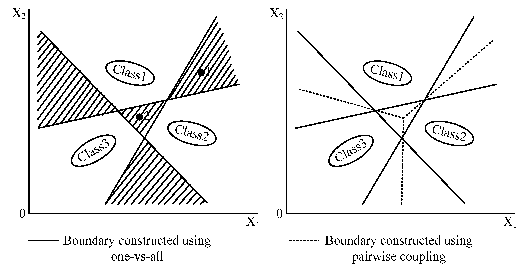
Traditionally, most of the existing classifiers are based on binary classification, which cannot adequately solve practical problems as real implementations always include multi-classification problems. Modifications should be made to the binary classifiers to entitle them with the probabilistic ability. The one-versus-all strategy is one of the solutions, which constructs a group of classifiers
lclass = [
C1,
C2,…,
Cd] in a
d-label classification problem. However, the classification accuracy is relatively poor because it employs only one threshold to separate the target group from the others which leaves large indecisive region, shown in
Figure 2. As a result, the 1vs1 strategy is adopted here, whose detailed definition is explained in reference [
25].
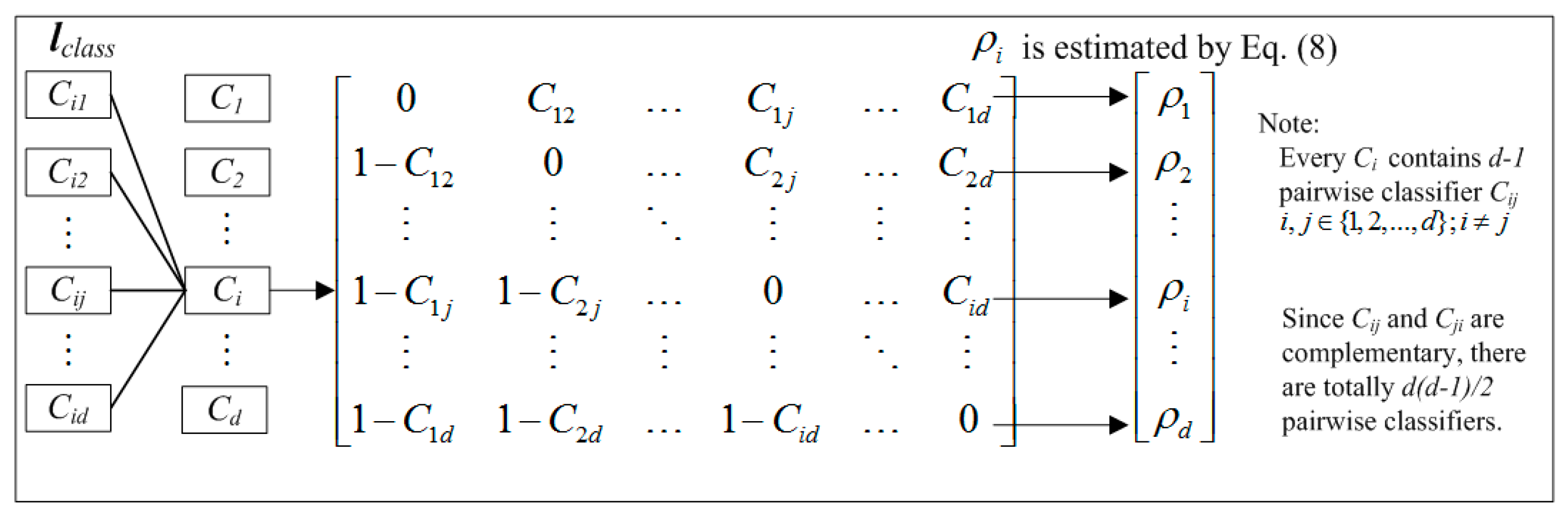
In a fault diagnosis process where there are
d possible faults,
lclass contains a set of pairwise coupling strategy
Cij as shown in
Figure 3. Then, the extracted feature vector
x will be processed and a probability vector
could be generated, Here,
denotes the probability and
x belongs to the
jth label for
j = 1 to
d. Therefore,
is an independent probability and
. The following pairwise coupling strategy for multi-classification is proposed. The independent probability
is calculated as
where
nij is the number of feature vectors.
Hence, the probability can be more accurately estimated from as the indecisive region between different thresholds in one versus all strategy is eliminated. For simplicity, the notation SBELM since then represented the proposed pairwise-coupled SBELM.


