Abstract
We present a computationally light real-time algorithm which automatically detects blinks, saccades, and fixations from electro-oculography (EOG) data and calculates their temporal parameters. The method is probabilistic which allows to consider the uncertainties in the detected events. The method is real-time in the sense that it processes the data sample-by-sample, without a need to process the whole data as a batch. Prior to the actual measurements, a short, unsupervised training period is required. The parameters of the Gaussian likelihoods are learnt using an expectation maximization algorithm. The results show the promise of the method in detecting blinks, saccades, and fixations, with detection rates close to 100 %. The presented method is published as an open source tool.
Introduction
Real-time monitoring of human physiology can provide relevant health and performance related metrics for various applications ranging from observing the physical status of a worker to monitoring the cognitive states of a user. As one such signal, eye movements serve as a rich source of contextual user-related information and electro-oculography (EOG) provides a light-weight, robust, and relatively non-intrusive means for measuring them. EOG signal is generated from the changes in the orientation of the corneo-retinal potential which can be measured with electrode-pairs on opposite sides of the eye. From this signal, fixations, saccades, and blinks can be detected.
While the spatial accuracy of EOG is appreciably lower than what is achievable with, e.g., videooculography (VOG), the typical EOG registration is run at considerably higher frame rates, allowing for various parameters of the eye to be computed accurately (Heide et al., 1999). Especially, the durations of saccades and different stages of a blink can be estimated with high precision. EOG has thus been utilized in many applications, such as monitoring sleepiness, tiredness, and fatigue (Ingre et al., 2006; Morris & Miller, 1996; Papadelis et al., 2007), detecting changes in cognitive workload (Ryu & Myung, 2005; Veltman & Gaillard, 1996), recognizing the context from gaze pattern behavior (Bulling et al., 2011), and even sleep stage classification (Virkkala et al., 2007).
Various methods for detecting saccades and blinks from eye movement signals exist. Some of the methods utilize VOG for obtaining the signal but the underlying principles could be applied to both EOG and VOG measurements. For instance, Engbert & Kliegl (2003), Engbert & Kliegl (2004), and Engbert & Mergenthaler (2006) make VOG measurements and Jammes et al. (2008) and Pettersson et al. (2013) make EOG measurements to detect saccades and/or blinks by using the derivative of the eye movement signal with various methods for determining the threshold; Behrens et al. (2010) consider the deviation of acceleration values from the EOG signal; Daye & Optican (2014) utilize sophisticated particle filtering for detecting the events in eye movement signal captured with VOG; Vidal et al. (2011) use a supervised kNN method to cluster data in the subspace formed by various features of EOG signals; and Niemenlehto (2009) uses constant false alarm rate detection method to detect events from the EOG signal. In addition, Czabański et al. (2013) and Pander et al. (2014) use fuzzy c-means clustering for detecting events from the clinical electronystagmus signal. However, these methods typically use a harsh threshold for detecting the events, focus either on blinks or saccades, use supervised learning, and/or are batch methods for offline processing.
In this paper, we present a probabilistic, computationally light real-time algorithm for automatically detecting blink, saccade, and fixation events from EOG data (here we assume that only blinks, saccades, and fixations occur). The method also calculates the temporal parameters (starts and durations) of the classified events. The method requires a short training period, during which samples of each class (fixations, blinks, and saccades) are present. However, the training is performed completely unsupervised and the class identities are automatically detected. To the best of our knowledge, the presented method is the first real-time probabilistic algorithm for detecting blinks, saccades, and fixation which uses unsupervised training.
To test the algorithm, we registered data in a simple task where the users were instructed to fixate on a dot on a display and shift their gaze when the dot jumped to another position on a varying screen distance. Occasionally between the saccades, the subjects were instructed to blink with a visual cue. The results show that the method is accurate in detecting the EOG events. In addition, the algorithm is fairly simple, making it robust and easy to implement. The method is published as open-source for anyone to use and amend.
Method
The EOG data contains horizontal and vertical signals which capture the eye movements in these directions. In our framework, each signal sample is assumed to be part of a saccade, blink, or fixation, and detecting, e.g., a saccade means that a sample (or sufficiently many successive samples) is being classified as a saccade. The detection method is probabilistic, assigning a probability for each sample as being one of these so that the probabilities always sum to unity. The approach resembles fuzzy clustering, used by, e.g., Pander et al. (2014), but a philosophical difference exists between the two as in fuzzy logic a sample belongs partly in many classes whereas in a probabilistic framework each sample can belong to only one class while there is a (subjective) probability about this belonging (Duda et al., 2000). The algorithm contains filtering, feature extraction, training, and actual event detection stages. It is described as pseudocode later in the text (in Algorithm 1).
Filtering
EOG data is inherently noisy (Heide et al., 1999). In order to increase the signal-to-noise ratio, the signals are filtered with a low-pass filter. When the cutoff frequency of the filter is decreased, the signal-to-noise ratio increases and the detection of the features gets easier. However, such heavy low-pass filtering smoothens the eye movement signal causing distortions to the temporal parameters (Jäntti et al., 1984). Hence, in order to compute the temporal values more accurately, the original signal should also be filtered with another filter with a higher cutoff frequency – resulting in two differently filtered signals (or four since there are vertical and horizontal signals).
Feature extraction
In order to use a classifier we must first have something to classify. For this, features are extracted from data. The features should be chosen such that the events to be classified differ as much as possible from each other in the feature space. Here, two features are used. The first one, denoted as Dn, is the norm of the derivative of the filtered horizontal and vertical EOG signals:
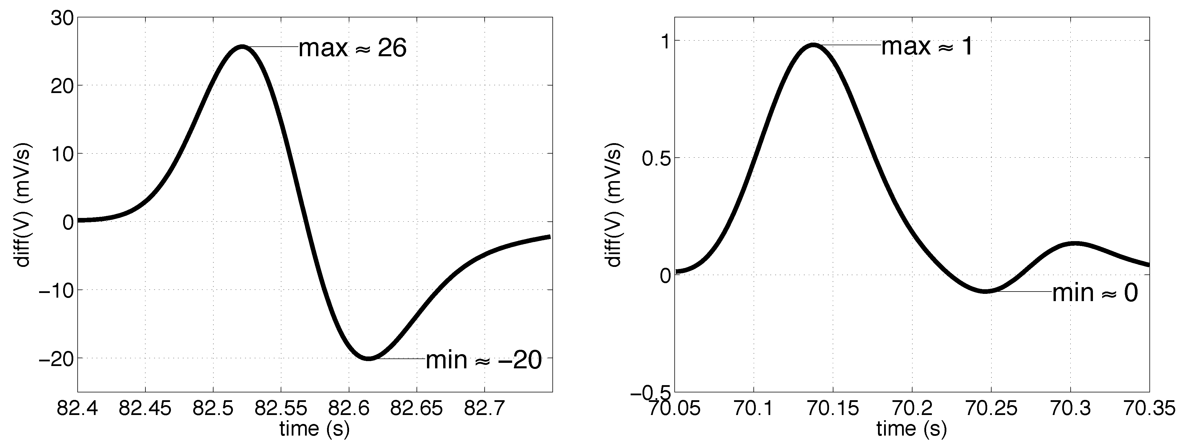
where H and V denote the horizontal and vertical components of the EOG signal. The rationale here is that for fixations, the norm is ideally zero (and in practice at the level of the noise of the signal) as a steady signal produces zero derivative. On the contrary, during saccades and especially blinks the value of the derivative is high. Hence, this feature is useful in separating fixations from blinks and saccades. The second feature, denoted as Dv, is used for separating blinks from saccades and is based only on the derivative of the vertical EOG signal. With the positive electrode for the vertical EOG located above the eye (signal level increases when the eyelid closes), the feature is defined as the difference between successive maxima (max) and minima (min) of subtracted with the absolute value of the sum of these:
If vertical EOG is registered with the electrode sites swapped, one simply needs to interchance the min and max in (2). The reason behind (2) is that a blink produces a distinctively symmetrical pattern in the derivative of the vertical signal and should thus have a higher value for Dv than a saccade (see Figure 1). For computing Dv, local maximum is stored and compared to the subsequent local minimum.

Figure 1.
An example of a first derivate of a filtered vertical signal during a blink (left) and a saccade (right). Note the difference in the amplitudes.
The probabilistic model
Let us denote a fixation, saccade, and blink with , , and , respectively. We are interested in the probability of an event given the observed data: , . As described above, the data is being “compressed” into two features (1) and (2), so that . Let us take the probability of an event being a fixation to be independent of so following the Bayes’ theorem we get
where in the normalization factor denotes a “non-fixation” event, i.e., an event which is a saccade or a blink. When forming the probability of a saccade, the “fixation / non-fixation” state is marginalized out so that
where the probability of observing a saccade given that we observe a fixation is trivially zero (p(s|f,D) = 0), the probability of observing a saccade given that we observe a non-fixation and the two features are dependent only on Dv (), and where the probability of observing a non-fixation given the data is simply
as they are complementary events. For blinks we get an equation similar to (4):
Hence, for each data sample we first compute the probability of it stemming from a fixation by extracting Dn and using (3) and then compute the probability of it stemming from a saccade or a blink by extracting Dv and using (5), (4), and (6).
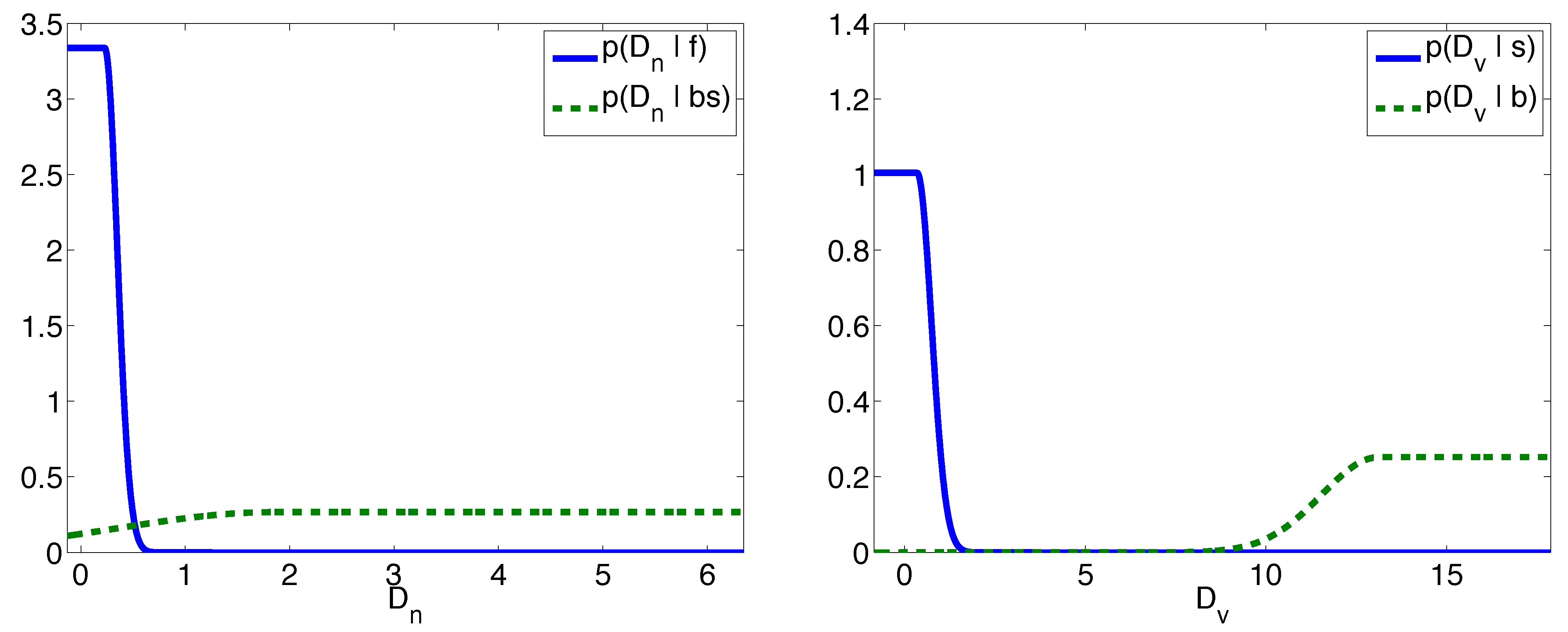
In order to implement the above formulas we must insert some probability distributions for the likelihoods p(Dn|f), , p(Dv|s), and p(Dv|b). A widely used and typically robust distribution is a Gaussian (The functional form of the Gaussian distribution is ) which is our choice although the actual distributions may not be exactly Gaussian; this issue is dealt with in Discussion. We set the distributions to be asymmetric Gaussians so that, for instance, if Dv exceeds the mean value for blinks (µb), which should always be higher than the mean value for saccades, the likelihood is the maximum value of the distribution:
Figure 2 shows the forms of the four likelihoods in Dn and Dv coordinates.
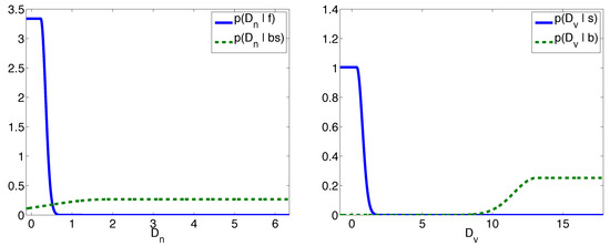
Figure 2.
Illustrative figures of the likelihoods in Dn and Dv coordinates. p(Dn|bs) denotes the likelihood p(Dn|). The parameters of these distributions were estimated from a training data that was used in the experiments.
Training
The learning scheme is unsupervised which means that the class identities of the training samples are unknown. The problem is thus to fit the likelihoods into the training data most optimally, that is, to find optimal values for the eight parameters of the Gaussian distributions – mean and variance for each of the four likelihoods – and the prior probabilities p(e).
For estimating these parameters we utilize the conventional method, the expectation maximization (EM) algorithm for Gaussian mixture model (GMM). The EM algorithm can be considered a probabilistic version of the classic Lloyd’s algorithm used to find k-means clustering. In brief, EM-GMM is an iterative method for unsupervised clustering of data in which the points are assumed to be members of Gaussian distributions (kernels) with unknown parameters (Bishop, 1995; Duda et al., 2000). The prior probabilities p(e) are the average posterior probabilities of each kernel, i.e., the membership weights computed by EM-GMM. When extracting the Dn features from the training data, only the values at local maxima are used. Moreover, the Dv values are extracted only for those peaks for which ; this ensures that the most probable event in this case is a saccade or a blink. The smaller of the two kernel mean values in the Dn space is taken to correspond to the fixation likelihood and in the Dv space to the saccade likelihood. An example of the estimated Gaussian parameters and the resulting likelihoods is given in Figure 2.
Detection
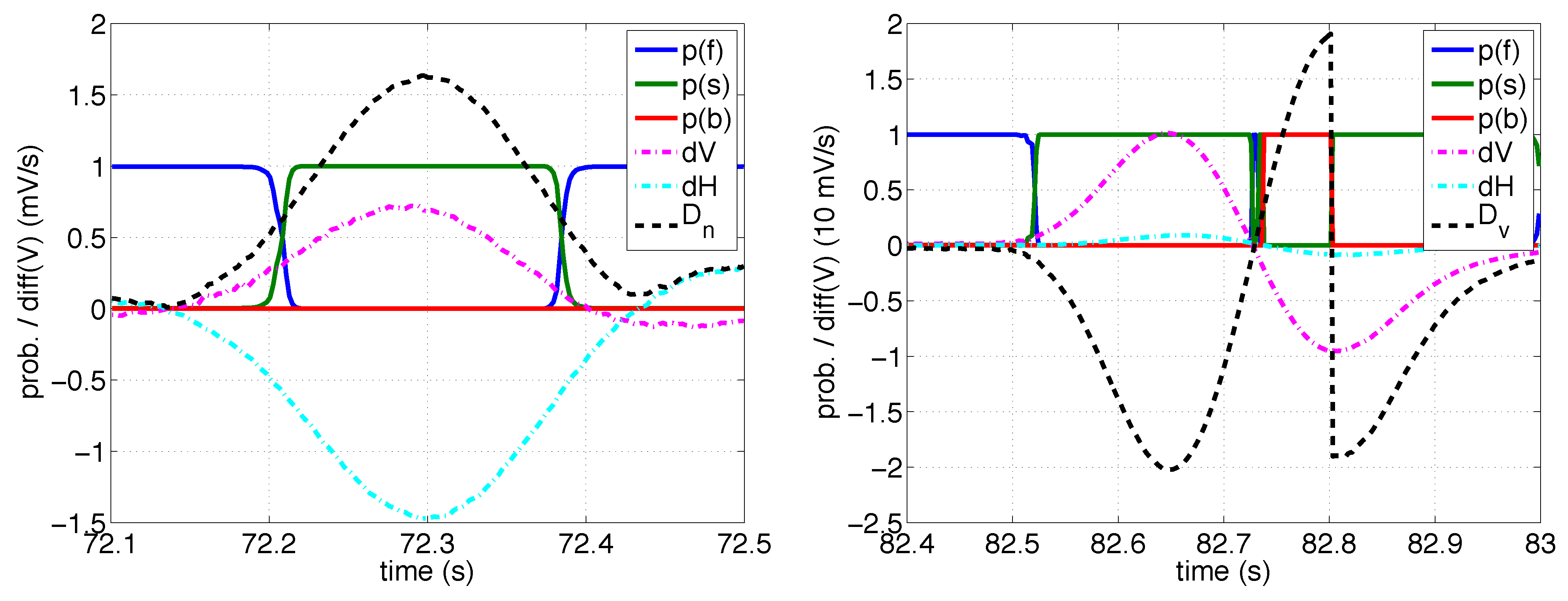
Having trained the model, that is, estimated the likelihood parameters and prior probabilities, each new sample of EOG signal can be classified. The method considers an event to occur as long as it has the highest probability. The start of a blink typically produces saccade samples since the Dv value increases from zero along the eyelid closing period and reaches the maximum value not until the eyelid is again opening at the fastest rate. Also, the samples after the minimum value of receive high probabilities for being saccade samples as the Dv value is low but Dn is high. Hence, a blink actually forms a saccade-blink-saccade sequence where the events overlap. From this it results that the blink can be detected (with high probability) only after its midpoint. There might also be a few fixation samples during the tiny moment when the eyelid is closed as Dn is low as well as few saccade samples after it before the Dv values get high enough for the samples to be classified as blink. To prevent the saccades ”framing” the blink sequences to be misclassified, they are abandoned if the next blink starts before they end or if the previous blink ends after they start. In addition, we set a minimum gap (e.g., 100 ms) between the ending of the previous saccade and the beginning of the next saccade and for the fixation probability mass between those. This also prevents double detection of dual saccades which may occur when a second saccade corrects the first (typically large) saccade which has missed a target slightly. Hence, there will be a slight delay as the saccade can be reported only when the minimum gap has elapsed since the ending of the saccade. Furthermore, we set a lower limit for the event durations and for the probability mass of the subsequent event samples because the noise in the signal may sometimes falsely produce spurious high probabilities for saccades or blinks. The computation of the event durations is described in the next Subsection. In Figure 3, a clip with a saccade and a blink and the corresponding probabilities are illustrated.
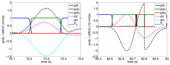
Figure 3.
Examples of signals produced by a saccade (left panel) and a blink (right panel). p(f), p(s), and p(b) refer to the posterior probabilities of a fixation, a saccade, and a blink; dV and dH refer to the first derivatives of the vertical and horizontal signals; Dn refers to the feature (1); Dv refers to the feature (2). Note the different scaling in the vertical axis in the right figure where the derivatives of the signals as well as the Dv values are divided by ten to have a better fit. The reader is referred to a color version for a decent viewing experience.
Computing the temporal values for the features
Once a saccade or blink is detected and estimated as completed, its temporal values can be estimated. For accurate estimates, we use signals that are filtered with the higher cutoff frequency. Previous values of Dn from this signal are constantly stored in a buffer whose length is defined as the maximum possible saccade length. For estimating the starting index, the buffer is explored from its maximum value towards its beginning and the sample point where the values start to increase is marked as the beginning of a saccade. Likewise, the ending of a saccade is found at the first zero crossing of the first derivative of the buffer that occurs after the buffer’s maximum value (see Figure 4 for an illustration). For estimating the exact temporal dimensions of a blink, two buffers are formed, the first from the vertical EOG signal (V) and the other from its first derivative. The length of the buffers are defined as the maximum blink length. The derivative values are explored from their maximum value (assuming that the vertical values increase when the eye looks down, that is, with the positive EOGv electrode above the eye) to the beginning and the point where the values go under one tenth of the maximum value is considered as the starting point of a blink. The midpoint of a blink is estimated as the point where the buffer of V values is at its highest and the duration of a blink is thus defined as two times the difference between midpoint and starting point. The temporal values and the computed features are illustrated in Figure 4.
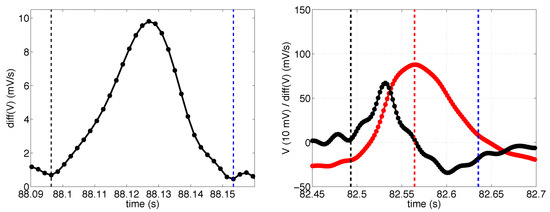
Figure 4.
Left: an example of the Dn feature (1) during a saccade. Right: an example of the vertical signal V (red line) and its derivative (black line) during a blink. Estimated points of beginning and ending of the events are marked with dashed lines (for the blink also the midpoint).
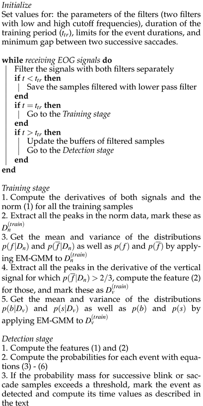
Algorithmic form
A practical realization of the method is presented as pseudocode in Algorithm 1. Matlab implementation of the algorithm is published online (see Additional information at the end of the text). Each detected event can be assigned a detection probability which can be, e.g., the highest or the average probability during the event.
| Algorithm 1 A practical realization of our blink and saccade detector method. |
 |
Experiments
While aiming to use our solution in non-controlled, natural viewing conditions, for evaluation purposes we need controlled experiments with known, triggered events.
Experimental setup
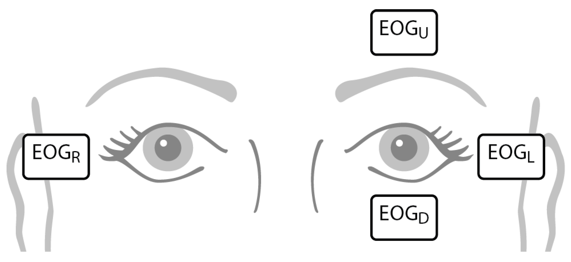
Data was recorded from five test subjects (1 male, 3037 years-old). All of the subjects had normal vision and did not report any health problems. The subjects were informed about the objectives and conditions of the study which complied with the Helsinki Declaration and was approved by the ethics committee of the Hospital District of Helsinki and Uusimaa, Finland. The attachment of the AgAg-Cl electrodes (Ambu, Ballenrup, Denmark) is illustrated in Figure 5. The electrode for the ground signal was attached on the left mastoid. For recording the signals we used a NeurOne amplifier (Mega Electronics Ltd., Kuopio, Finland) with a sampling rate of 500 Hz, alternating current (AC) measurement, and a lowpass filter whose cutoff frequency was set at 125 Hz (this device’s internal filter is not to be confused with the two filters used in the filtering stage of the algorithm). During registration, the signal was high-pass filtered with the NeurOne device’s default high pass filter (-3 dB at 0.16 Hz).
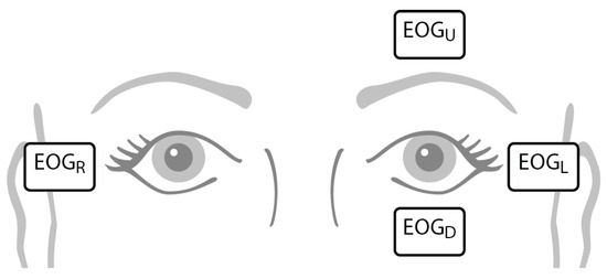
Figure 5.
The configuration of the electrodes used in the experiments.
As training data for the method, an image was shown to the subjects for one minute prior to the actual experiment. The image – which is shown in Figure 6 – contains five black dots whose size was one degree of the viewing angle. The subjects were instructed to fixate the dots for random durations and in random order and to blink whenever they felt like it (however, multiple times during the one minute). As the method is unsupervised, the times of the occurrence of the events was not needed. An example of the estimated Gaussian parameters and the resulting likelihoods from the training data of measurement M1 is given in Figure 2. The distance from the test persons’ eyes to the display was fixed to 80 cm in every part of each experiment.
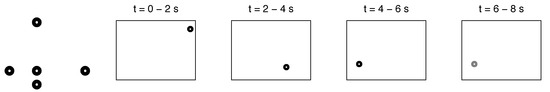
Figure 6.
Left: The training pattern used in the experiments. The images right from the training pattern illustrate the progress of the 8-second long test stimulus sequence of experiment 1. Note that each dot location in each sequence was different. Each last two seconds of the sequence is dedicated to a blink. None of the images is in scale.
For testing the performance, we used two different schemas, with fixed and randomized saccade intervals. The experiment with fixed saccade intervals was used to evaluate the performance as function of saccade angles whereas the purpose of the experiment with random saccade intervals was to mimic more natural viewing. In both experiments, the subjects were instructed to fixate a black dot, whose size was again one degree, which occasionally shifted to random locations. After every third saccade, the dot changed its color to gray, instructing the subject to blink. After the blink stimulus the dot stayed at the same location for two more seconds so the stimuli formed a repetitive saccadesaccade-saccade-blink sequence (however, with different dot locations in each sequence). The scale of the training pattern was different between the experiments; the largest distance between two adjacent dots, that between the rightmost and topmost dot, corresponded to a viewing angle of 7.1 degrees in experiment 1 and 17.5 degrees in experiment 2.
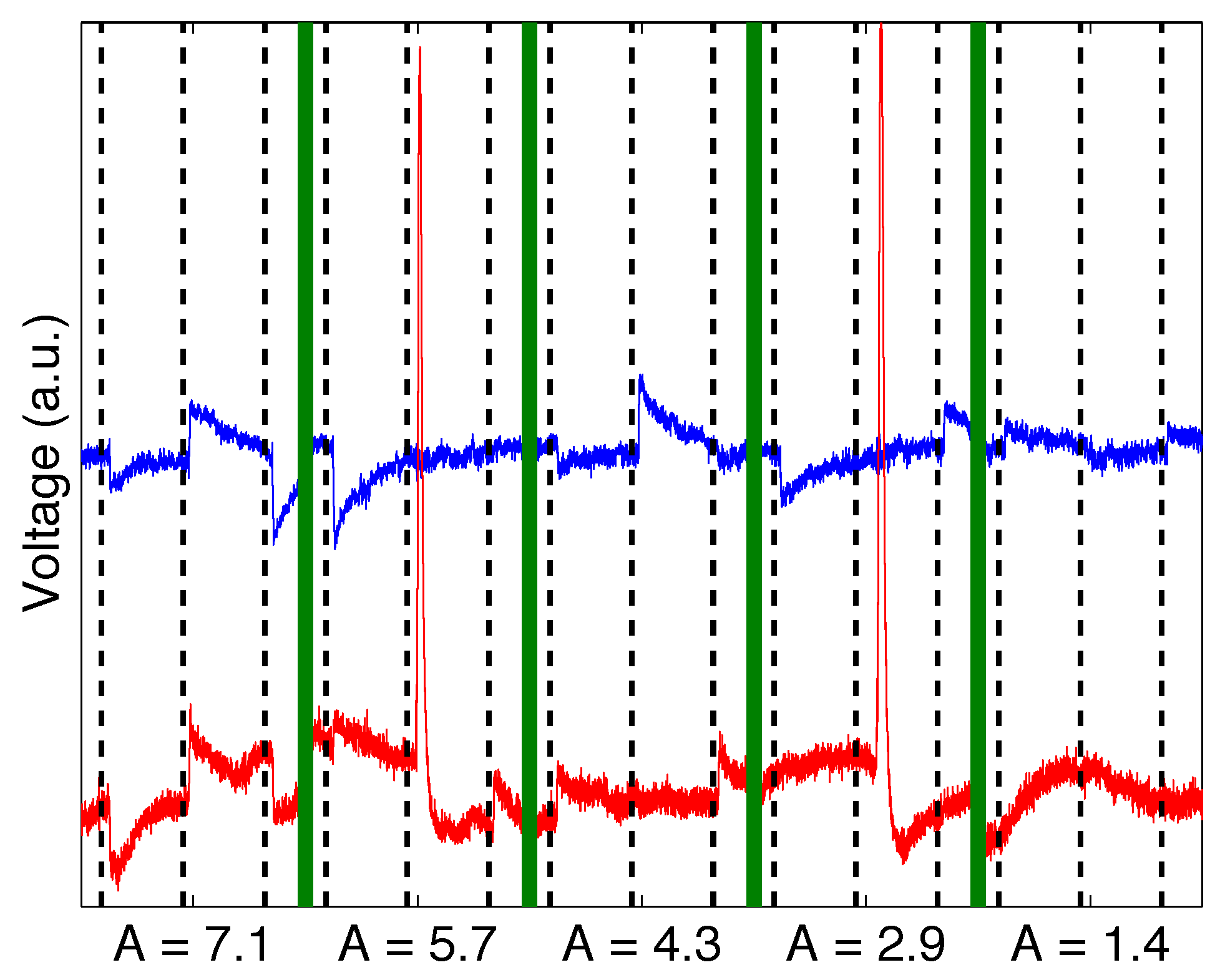
In experiment 1, the dot shifted to new location every two seconds, making the saccade-saccade-saccadeblink sequence last eight seconds (see Figure 6). The on-screen distance of the transitions of the dot was 10 cm for the first minute and then decreased for 2 cm after each subsequent minute until it was 2 cm. Assuming the gaze vector to be perpendicular to the screen plane the corresponding stimulus angles were 7.1, 5.7, 4.3, 2.9, and 1.4 degrees. The testing stage thus lasted five minutes during which 111 saccade stimuli and 37 blink stimuli were presented. For two of the five test subjects, experiment 1 was conducted twice on separate days, making the total number of measurements seven. Thus, the total number of saccade and blink stimuli were 777 and 259. In the results, these measurements are referred as M1,...,M7. Example clips of each five stimulus angles are shown in Figure 7. Note how the saccades of two smallest angles, especially 1.4 degree, are difficult to separate from the noise level of the signals, at least visually.

Figure 7.
A cascade of five example clips of raw EOG signals from different parts of experiment 1. The horizontal signal is shown in blue (on top) and the vertical in red (on bottom). The thick green vertical lines depict the border between the clips and the black dash lines indicate the occurrences of the stimuli. The labels in the x axis refer to the corresponding saccade angle (in degrees) of the clip. There are two blinks in the cascade, during the clips A=5.7 and A=2.9.
Experiment 2 was similar to experiment 1 except for the duration of the period that the dot stayed unchanged which was randomized with uniform distribution between 0.5 and 3.5 seconds and for the saccade angles which were also randomized between 2.2 and 35.7 degrees. This setting should better correspond to natural viewing. The seed for the random number generator was fixed to achieve comparable stimulus sequence. The second experiment was conducted with four test subjects (a subset of the five subjects that were used in experiment 1); these measurements will be referred as M8,...,M11.
Since the actual blink events may not always follow the stimuli, due to the subject missing a blink or making an extra blink, the midpoint of each blink was manually scored from the EOG data by one of the writers of this article (who was not involved in making the analysis) according to the AASM Manuals for the Scoring of Sleep and Associated Events (Iber et al., 2009). We assume that this manually scored reference midpoint of each blink is between the beginning and ending timestamps that were detected by the method. For saccades, we rely on the timestamped stimuli and assume that saccades start within 0.5 s (1.0 s in experiment 2) after the dot has switched location. The reference fixation period, defined as a period during which there should be no blinks nor saccades, is taken to be the time between the ending of a previous event window and beginning of the next one; the saccade window was taken to begin from the saccade stimulus onset and end after 0.5 s (1.0 s in experiment 2) whereas the blink window was taken to begin 0.5 s before the manually scored midpoint and end 0.5 s after the midpoint.
The method contains only a few parameters. In these experiments, the signals were filtered (after being lowpass filtered inside the measurement device with 125 Hz cutoff frequency) with two separate 150th order Butterworth low-pass filters with cutoff frequencies at 1 Hz and 40 Hz. The filter with the lower cutoff frequency was used for computing the features of the signals whereas the other filter was used for computing the temporal values. The minimum and maximum blink durations were 30 ms and 500 ms and the minimum and maximum saccade durations were 10 ms and 150 ms. These figures reflect typical durations for spontaneous blinks and saccades (Holmqvist et al., 2011). The minimum gap between two successive saccades was set to 100 ms, unless otherwise noted. For clarity, the values of these parameters are tabulated in Table 1. For simplicity, the estimated detection probabilities were not utilized in evaluating the performance (that is, the classifier was binary here, reporting either detection or no-detection).

Table 1.
The parameter values used in the experiments.
For measurement M4 of experiment 1 (see Table 2 and Table 3), we discarded the last 40 seconds of data due to the eyes of the subject drying, causing her to close her eyes. No other data was discarded.
Table 2.
The detection rates for blinks in experiment 1 for each measurement and their mean and median values.
Table 3.
The detection rates for saccades in experiment 1 as function of the saccade stimulus angle, for each measurement, and their mean and median values.
Performance measures
For evaluating numerical detection figures we used the conventional true positive rates (TPR), also known as sensitivity or recall, and positive predictive values (PPV), also known as precision, defined as
where TP indicates the number of true positives, i.e., the correctly identified events, Ntrue is the total number of true events, and Nmethod is the total number of events detected by the method. Hence, a method that, e.g., detects blinks whenever there was a blink but also detects false blinks (i.e., false positives) has a high TPR but low PPV whilst a method that detects only a few blinks has high PPV but low TPR. For an ideally performing method both rates would be 100 %. The TPR and PPV values can be combined as their harmonic mean, i.e., the F-score, defined as
For fixations, Nmethod was computed as the sum of false and true positives, where a false positive occured when there was no blink nor saccade when there should have been a blink or a saccade.
Results
Experiment 1
The detection rates for blinks in experiment 1 are given in Table 2 demonstrating the high performance in detecting blinks. The mean duration of the detected blinks was 183reported in literature ± 53 ms which is in line with the values (Caffier et al., 2003; Holmqvist e al., 2011; Stern et al., 1984).
The detection rates for saccades and fixations are tabulated in Table 3 and Table 4 for each saccade stimulus angle. The rates for saccades are high for all but the smallest angles and the decrease of PPV of fixations is due to increase in Nmethod, caused by misdetected saccades with small angles. Saccades with the smallest angles are more difficult to detect as the signal generated by these is hard to differentiate from the ambient noise level of the signal (as can be seen from Figure 7).
Table 4.
The detection rates for fixations in experiment 1 as function of the saccade stimulus angle, for each measurement, and their mean and median values.
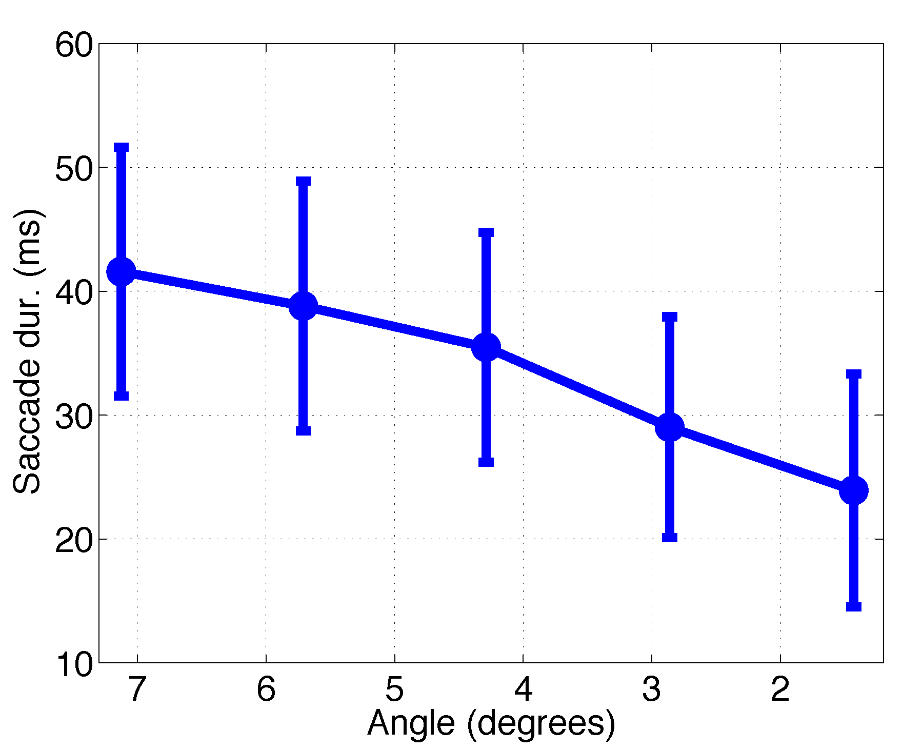
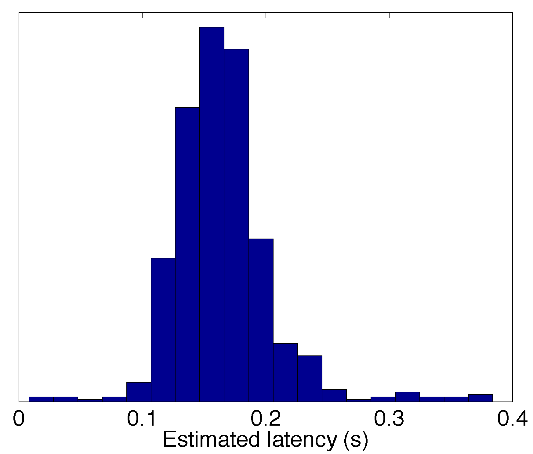
To demonstrate the decrease in the performance of the method to detect saccades as function of the stimulus angle visually, the F-score is plotted in Figure 8. Saccades above four degrees are detected reliably. With saccades of three degrees the method performs adequately, whereas saccades below two degrees cannot be detected. The estimated durations of the saccades as function of the stimulus angle are illustrated in Figure 9. Again, the durations coincide with those found in literature (A. Bahill et al., 1981; T. Bahill & Stark, 1977; Becker & Jürgens, 1990), especially with the ”duration = 2.2 × amplitude + 21” relation, suggested by Carpenter (1988). A histogram of the estimated latencies, that is, the lags of the saccade starting times estimated by our algorithm compared to the stimulus times, is depicted in Figure 10 which shows that the subjects indeed made the saccades within the 0.5 s time window after the stimulus was shown, with the mode of the latencies at 150ms.
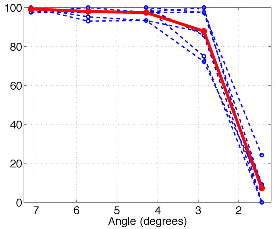
Figure 8.
The F-scores of the saccades in experiment 1 as function of the stimulus angle. The blue dashed lines show the scores for each measurements whose mean is depicted with the solid red line.

Figure 9.
The saccade durations (mean ± std) in experiment 1 as function of the stimulus angle.

Figure 10.
A histogram of the estimated latencies of all the observed saccades in experiment 1 (N = 649).
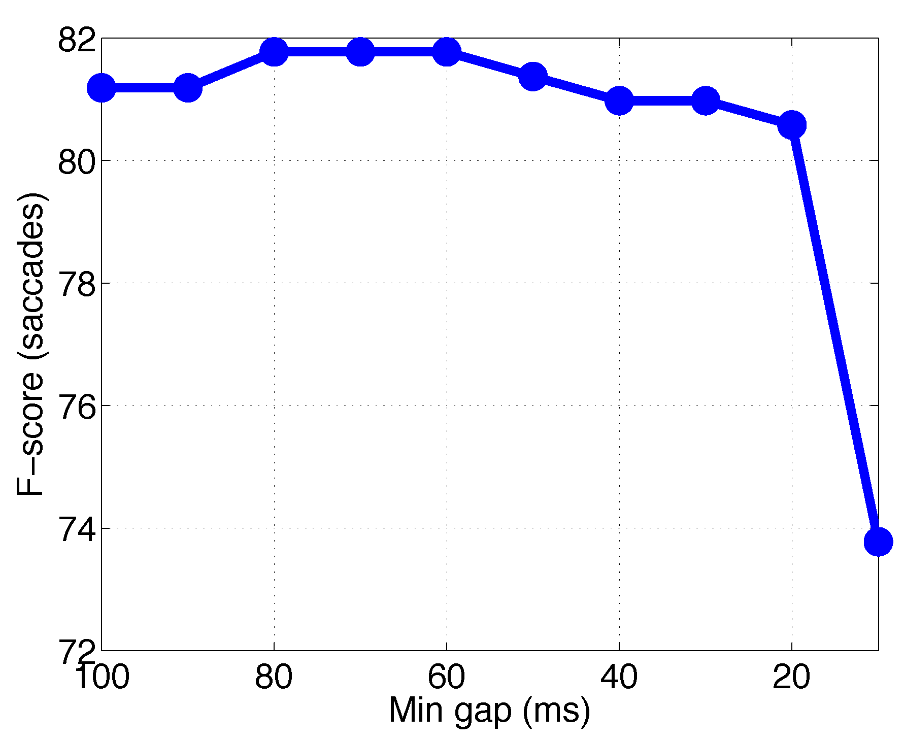
We originally set the minimum gap between two successive saccades in the algorithm at 100ms. However, as this setting might miss nearby actual saccades in natural viewing conditions, we investigated the effect of decreasing the minimum gap. We re-computed the detection rates for measurement M2 (since it performed worst) with stepwise reduction of the minimum gap from 100 ms to 10 ms. The results are presented in Figure 11 which shows that the minimum gap has no significant effect on the performance of the method when the gap is set above 30 ms.
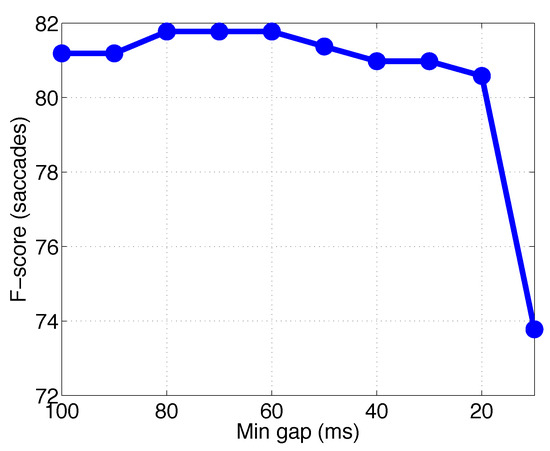
Figure 11.
The F-scores for saccades of measurement M2 (in experiment 1) as function of the minimum gap between two successive saccades.
Another interesting parameter to vary is the length of the training period. For this experiment we chose measurement M6 since it contained many blinks during the training period. Figure 12 shows how the Fscores for blinks and saccades (over all the saccade angles) vary as the length is shortened from 60 seconds to 5 seconds with 5 seconds step. According to the figure, the detection performance is constant as long as the duration of the training period exceeds approximately 10 seconds. The first five seconds of the data contains only a single blink into which a distribution (with positive variance) is impossible to fit.
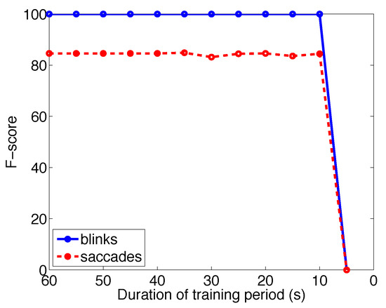
Figure 12.
The F-scores for saccades and blinks of measurement M6 (in experiment 1) as function of the length of the training period.
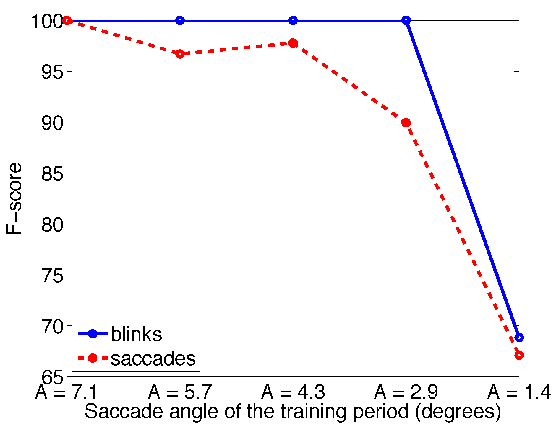
Finally, we studied the influence of training the system with a different saccade angle than used for testing. For this, we chose measurement M7 and discarded its initial training period (with which the F-score was 100 %). Instead, we used each of its five one-minute clips in turn as training period and used the algorithm to classify the events in the rest of the one-minute clips. This way, each of the training data sets corresponded to different saccadic angles. To make the comparison fair, the test data contained only three largest saccade angles. The result is illustrated in Figure 13 which shows that when using the smallest angle saccade stimulus data as training data the detection is understandably poor. For angles above this, the performance for blinks is perfect whereas for saccades the detection rates reach 100 % when the training data contains the largest saccade angle.
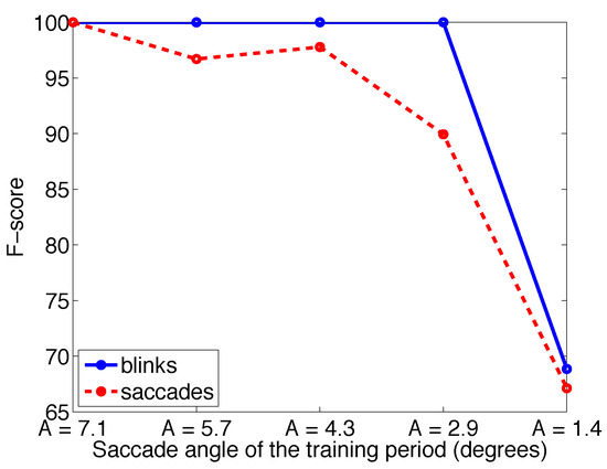
Figure 13.
The F-scores for saccades and blinks of measurement M7 (in experiment 1) as function of the saccade angle of the training period.
Experiment 2
In conducting experiment 2, all the model parameters were the same as in experiment 1. However, we had to change the acceptance window between the onsets of stimulus and an assumed saccade because the latencies here were naturally slower than in experiment 1 as the reaction times to variable non-predictable stimulus shifts increased. Hence, we increased the window for automatically associating a saccade with a temporal trigger defining stimulus onset (that is, associating stimulus-response pairs) to one second (it was 0.5 seconds in experiment 1).
The results of experiment 2 are tabulated in Table 5. Blinks seem to be detected with approximately the same accuracy as in experiment 1. The TPR values being lower than 100 % can be probably attributed to small saccade angles involved in the experiment whereas the PPV values being lower than 100 % is probably due to the sporadic behavior with occasionally very fast (⇠0.5 s) stimulus location changes causing subjects to make additional corrective saccades.
Table 5.
The detection rates for blinks, saccades and fixations in experiment 2 for each measurement, and their mean and median values.
Comparison with other methods
Comparing with existing algorithms is somewhat challenging because of the lack of standardized performance metrics, public datasets, and published algorithm codes. To alleviate future comparison, we have published our algorithm code online (see Additional information at the end of the text).
Behrens et al. (2010) report on an improved algorithm for automatic saccade detection in EOG data using adaptive thresholding automatically calculated during the measurement. However, they fail to report any performance figures, only providing demonstrative plots of the algorithm at work over two separate use cases (driving a car and microsleep detection). Jammes et al. (2008) reported on a blink detection algorithm intended for drowsiness detection employing empirically selected threshold values based on calibration EOG recordings. The algorithm’s performance was compared to manually processed EOG data over 30 hours and the TPR values among test subjects were between 95.9 and 99.8 % and the PPV values between 98.0 and 100.0 %. Daye & Optican (2014) introduce a method for saccade detection using a particle filter as a Bayesian estimator. Their method removes the baseline velocity component of the eye movement signal and they claim that this allows for reliable detection using a fixed threshold. While the method is able to perform the analysis online, they admit that it has a high computational burden. They do not report detection rates but instead provide a noise sensitivity analysis for temporal performance values over a generated eye movement signal, exemplary signal plots in various applications, and report that the algorithm ”detected all the saccades in the trial despite the wide range of amplitudes”. Vidal et al. (2011) report on their work toward an online detection algorithm for eye movements based on EOG signal features. They conclude that the performance of their k-nearest-neighbour classifier is above 80% for both precision and recall. Bulling et al. (2011) reported F-scores for their offline method for detecting blinks and saccades (angle not given), both of which were 94 %. The value, however, was a maximum over a parameter sweep and may hence be overfitted to the training data; for novel test data, the value is likely to be smaller. The saccade detector of Niemenlehto (2009) report F-scores for simulated data up to 95.5 %, depending on the parameter value and the noise level. Pettersson et al. (2013) detect saccades and blinks offline. For saccades of 5 and 7.5 degrees they report the mean TPR value to be 95.5 % and for blinks they report the TPR value to be 97 % while having PPV at 94 %.
Our method performs at least equally well with the referenced methods above. For blink detection, our average TPR, PPV, and F-score values were 99.6, 98.9, and 99.2 % for experiment 1 and 99.2, 95.3, and 97.2 % for experiment 2. For saccades, the results depend on the saccade stimulus angle; for angles 7.1, 5.7, and 4.3 of experiment 1, the average F-scores were 99.3, 98.0, and 97.4. For detailed results, see Table 2 and Table 3. In experiment 2, the average TPR, PPV, and F-score values for saccades were 93.0, 87.5, and 90.2 %.
Table 6 shows a qualitative comparison between the current method and earlier work referenced above. Despite having performance similar to that of the reference methods, our method has several advantages which many of the reference methods lack. 1) As opposed to batch methods, the real-time feature of the method allows for real-time monitoring of, e.g., human physiology which can provide relevant health and performance related metrics. 2) The unsupervised learning period that we use should only contain examples of each event type without manually labeled data. This allows for running studies in natural environments with no pre-set instructions or calibration sequences – almost any short patch of natural viewing data should provide the necessary blinks, saccades, and fixations. 3) Our method assigns a detection probability for each event which can be, e.g., the highest or the average probability during the event. Unlike a binary classifier, such probabilistic approach enables the consideration of uncertainties in classification when making decisions based on the detected events. For instance – when classifying data between three conditions: blinks, saccades, and fixations – two blinks, one detected with a 34 % and one with 100 % probability might both be crudely classified as blinks with a binary classifier if the blink with 34% probability is the most likely event out of the three possibilities. 4) Many of the referenced methods focus on either blinks or saccades; we detect both of these, as well as fixations, with the same algorithm. To the best of our knowledge, the presented method is the first published method that 1) is realtime, 2) uses unsupervised training, 3) is probabilistic, and 4) detects blinks, saccades, and fixations. In addition, our method is computationally light. Finally, one more advantage of our probabilistic model is the small number of parameters (only the mandatory filter parameters, thresholds for event durations, the minimum gap between saccades, and the duration of the training period) of which the last two are likely to have largest effect on the performance but as the results demonstrate, the F-scores were not sensitive to these parameters. This implies that the method should be robust and the detection rates are likely to be equally good in other conditions, too.
Table 6.
A qualitative comparison between various methods. The features ’b’, ’s’, and ’f’ refer to blinks, saccades, and fixations. In the column ’other features’, (*) refers to activity recognition, (**) to smooth pursuit, and (***) to smooth pursuit, vergence, and vestibulo-ocular reflex. The ’-’ mark in the column describing the computational load indicates that the load is unknown. R-T refers to real-time (if ’no’, the method is a batch method).
Discussion
The likelihood distributions were taken to be (asymmetrical) Gaussians but there is no guarantee that natural blinks and saccades follow a Gaussian distribution in our chosen feature space. However, the Gaussian distribution is typically a robust model and the results of this paper justify the choice. We tried log-normal distribution for the likelihoods in the Dv space but with inferior results. Nevertheless, future work might include testing with other distributions to gain even better performance.
The results indicate that the angles of the saccades to be detected do not need to be same as those used for training the system. In addition, although our training period lasted one minute, clearly shorter periods resulted in equally good results as long as the training data contained at least two examples of each class. As for possible future development of the system, the EMGMM algorithm could be implemented as a recursive version resulting in a truly online model which would update itself after each observation. In this scenario there would be no separate training period but the estimation of the parameters of the model would improve over time.
We originally set the minimum distance between two successive events as 100ms. We experimented with setting the threshold lower and as Figure 11 shows, this had no adverse effects on recognition performance. In natural viewing conditions, a high threshold may lead to the method misclassifying actual events such as express, anticipatory, or corrective saccades (Becker & Fuchs, 1969) with short latencies.
The introduced model assumes only one event to occur at a time so that the sum of the probabilities of the three classes is always unity (and ideally one of the probabilities is unity). However, in reality blinks and saccades may overlap. These situations might be handled by assuming that simultaneously observing approximately 50 % probability for both saccade and blink indicates such hybrid event; testing this schema is left for future work.
The task design of experiment 1 had two issues. i) There was a constant two-second interval between stimulus shifts without any jitter. The subjects can quickly learn to anticipate the following shift, which in turn might lead to anticipatory saccades with noticeably shorter reaction times. Therefore we conducted experiment 2 with randomized intervals. ii) Another possible issue was the use of constant stimulus shift angles in each one-minute window which could result in a time-on-task effect to affect the subjects’ performance. However, as the total test time was only five minutes and the rate of detected blinks was constant throughout, this does not appear to affect the performance. Hence, the effect of worse classification performance for saccades later in the series can be attributed in whole to the smaller saccade angles and therefore smaller signal amplitudes.
In this paper, we have presented a probabilistic realtime algorithm for detecting blinks, saccades, and fixations from EOG signals. The algorithm uses unsupervised training. According to the results, the method is well capable of detecting blinks, fixations, and saccades of any direction with angles above three degrees and to estimate the temporal values of these with high accuracy.
Additional Information
A Matlab implementation of the algorithm is available online in https://github.com/bwrc/eogert, with which the signal is processed quicker than recorded (with a sampling rate of 500 Hz) and the estimation of the likelihood parameters with EM-GMM takes less than ten seconds (on a Linux Ubuntu with a 2.60 GHz processor). Additionally, the method will be implemented in Python as open source software and distributed under the MIT License as a module for the MIDAS (Modular Integrated Distributed Analysis System) framework, allowing integration of on-line analysis of streaming psychophysiological signals into applications. The MIDAS framework is developed at our Research Centre and is available at http://www.github.com/bwrc/midas.
Acknowledgments
The study was supported by the Academy of Finland Grant 264653. The authors thank Doctor Käi Puolamaki for valuable comments on the manuscript.
References
- Bahill, A., A. Brockenbrough, and B. Troost. 1981. Variability and development of a normative data base for saccadic eye movements. Investigative Ophthalmology & Visual Science, 116–125. [Google Scholar]
- Bahill, T., and L. Stark. 1977. Oblique saccadic eye movements. Arch Ophthalmol 95. [Google Scholar]
- Becker, W., and A. F. Fuchs. 1969. Further properties of the human saccadic system: eye movements and correction saccades with and without visual fixation points. Vision research 9, 10: 1247–58. [Google Scholar]
- Becker, W., and R. Jürgens. 1990. Human oblique saccades: quantitative analysis of the relation between horizontal and vertical components. Vision Research 30, 6: 893–920. [Google Scholar] [PubMed]
- Behrens, F., M. MacKeben, and Schröder-Preikschat. 2010. An improved algorithm for automatic detection of saccades in eye movement data and for calculating saccade parameters. Behavior Research Methods 42, 3: 701–708. [Google Scholar] [PubMed]
- Bishop, C. M. 1995. Neural networks for pattern recognition. Clarendon press Oxford. [Google Scholar]
- Bulling, A., J. A. Ward, H. Gellersen, and G. Troster. 2011. Eye movement analysis for activity recognition using electrooculography. Pattern Analysis and Machine Intelligence, IEEE Transactions on 33, 4: 741–753. [Google Scholar]
- Caffier, P., U. Erdmann, and P. Ullsperger. 2003. Experimental evaluation of eye-blink parameters as a drowsiness measure. European Journal of Applied Physiology 89, 3-4: 319–325. [Google Scholar]
- Carpenter, R. H. 1988. Movements of the eyes, 2nd rev. ed. Pion Limited. [Google Scholar]
- Czabański, R., T. Pander, K. Horoba, and T. Przybyła. 2013. Fuzzy clustering based methods for nystagmus movements detection in electronystagmography signal. Journal of medical informatics technologies 22. [Google Scholar]
- Daye, P. M., and L. M. Optican. 2014. Saccade detection using a particle filter. Journal of neuroscience methods 235: 157–168. [Google Scholar]
- Duda, R. O., P. E. Hart, and D. G. Stork. 2000. Pattern classification. Wiley-Interscience. [Google Scholar]
- Engbert, R., and R. Kliegl. 2003. Microsaccades uncover the orientation of covert attention. Vision Research 43, 9: 1035–1045. [Google Scholar]
- Engbert, R., and R. Kliegl. 2004. Microsaccades keep the eyes’ balance during fixation. Psychological science 15, 6: 431–436. [Google Scholar] [CrossRef]
- Engbert, R., and K. Mergenthaler. 2006. Microsaccades are triggered by low retinal image slip. Proceedings of the National Academy of Sciences of the United States of America 103, 18: 7192–7197. [Google Scholar] [PubMed]
- Heide, W., E. Koenig, P. Trillenberg, D. Kömpf, and D. Zee. 1999. Electrooculography: technical standards and applications. Electroencephalogr Clin Neurophysiol Suppl 52: 223–240. [Google Scholar]
- Holmqvist, K., M. Nyström, R. Andersson, R. Dewhurst, H. Jarodzka, and J. Van de Weijer. 2011. Eye tracking: A comprehensive guide to methods and measures. Oxford University Press. [Google Scholar]
- Iber, C., S. Ancoli Israel, A. L. Chesson, and S. F. Quan. 2009. The AASM manual for the scoring of sleep and associated events. American Academy of Sleep Medicine. [Google Scholar]
- Ingre, M., T. Akerstedt, B. Peters, A. Anund, and G. Kecklund. 2006. Subjective sleepiness, simulated driving performance and blink duration: examining individual differences. Journal of Sleep Research 15, 1: 47–53. [Google Scholar] [CrossRef]
- Jammes, B., H. Sharabty, and D. Esteve. 2008. Automatic EOG analysis: A first step toward automatic drowsiness scoring during wake-sleep transitions. Somnologie Schlafforschung und Schlafmedizin 12, 3: 227–232. [Google Scholar] [CrossRef]
- Jäntti, V., I. Pyykkö, M. Juhola, J. Ignatius, G.-A. Hansson, and N.-G. Henriksson. 1984. Effect of filtering in the computer analysis of saccades. Acta Otolaryngol 96, s406: 231–234. [Google Scholar] [CrossRef] [PubMed]
- Morris, T. L., and J. C. Miller. 1996. Electrooculographic and performance indices of fatigue during simulated flight. Biological Psychology 42, 3: 343–360. [Google Scholar] [CrossRef]
- Niemenlehto, P.-H. 2009. Constant false alarm rate detection of saccadic eye movements in electro-oculography. Computer methods and programs in biomedicine 96, 2: 158–71. [Google Scholar] [CrossRef]
- Pander, T., R. Czabański, T. Przybyła, and D. Pojda-Wilczek. 2014. An automatic saccadic eye movement detection in an optokinetic nystagmus signal. Biomedical Engineering/Biomedizinische Technik. [Google Scholar]
- Papadelis, C., Z. Chen, C. Kourtidou-Papadeli, P. D. Bamidis, I. Chouvarda, E. Bekiaris, and N. Maglaveras. 2007. Monitoring sleepiness with on-board electrophysiological recordings for preventing sleep-deprived traffic accidents. Clinical Neurophysiology 118, 9: 1906–1922. [Google Scholar]
- Pettersson, K., S. Jagadeesan, K. Lukander, A. Henelius, E. Haeggström, and K. Müller. 2013. Algorithm for automatic analysis of electro-oculographic data. Biomedical engineering online 12, 1: 110. [Google Scholar] [PubMed]
- Ryu, K., and R. Myung. 2005. Evaluation of mental workload with a combined measure based on physiological indices during a dual task of tracking and mental arithmetic. International Journal of Industrial Ergonomics 35, 11: 991–1009. [Google Scholar]
- Stern, J., L. Walrath, and R. Goldstein. 1984. The endogenous eyeblink. Psychophysiology 21, 1: 22–33. [Google Scholar] [PubMed]
- Veltman, J., and A. Gaillard. 1996. Physiological indices of workload in a simulated flight task. Biological psychology 42, 3: 323–342. [Google Scholar]
- Vidal, M., A. Bulling, and H. Gellersen. 2011. Analysing EOG signal features for the discrimination of eye movements with wearable devices. In Proceedings of the 1st international workshop on pervasive eye tracking & mobile eye-based interaction-petmei ’11. ACM Press: p. 15. [Google Scholar]
- Virkkala, J., J. Hasan, A. Värri, S.-L. Himanen, and K. Müller. 2007. Automatic sleep stage classification using twochannel electro-oculography. Journal of neuroscience methods 166, 1: 109–15. [Google Scholar]


Copyright © 2015. This article is licensed under a Creative Commons Attribution 4.0 International License.