Abstract
We analyze the feasibility of a cheap eye-tracker where the hardware consists of a single webcam and a Raspberry Pi device. Our aim is to discover the limits of such a system and to see whether it provides an acceptable performance. We base our work on the open source Opengazer (Zielinski, 2013) and we propose several improvements to create a robust, real-time system which can work on a computer with 30Hz sampling rate. After assessing the accuracy of our eye-tracker in elaborated experiments involving 12 subjects under 4 different system setups, we install it on a Raspberry Pi to create a portable stand-alone eye-tracker which achieves 1.42° horizontal accuracy with 3 Hz refresh rate for a building cost of €70.
Introduction
Recent advancements in eye-tracking hardware research have resulted in an increased number of available models that have improved performance and that provide easier setup procedures. However, the main problem with these devices continues to be the scalability since their price and the required expertise for operation make them infeasible at the large scale.
These latest commercial models provide great accuracies (between 0.1 and 1°) at high frequencies (over 100Hz); however, in situations where such accuracies are not necessary and such frequencies are irrelevant, their high prices make them unsuitable. For example, in the case of online advertisement, eye-tracking is used to analyze which parts of webpages draw more attention and how the page layout directs user gaze. In such a use case, even 10Hz data with an accuracy between 1–2° would be enough to generate the expected heatmap output.
In this work, we aim to build a cheap, open source alternative that works on a hardware setup common in consumer environments: a camera and an electronic device display. We believe that a system that provides comparable performance at an acceptable frequency will enable many applications on devices ranging from computers to tablets and smartphones.
Related Work
Appearance Based Methods
Eye-tracking methods which do not need IR equipment make use of regular commercial cameras, or sometimes even webcams. Common tasks in these trackers are head and eye localization, calibration and gaze estimation. Appearance based methods are one sub-class of these methods and use the eye appearance (i.e. pixel data or extracted features) to train a mapping for gaze estimation. They differ from the model based techniques that try to fit a 2D or 3D model to the subject’s face or eyes, in order to calculate the gaze point geometrically (Hansen & Ji, 2010).
One popular mapping method used in appearance based gaze estimation is Artificial Neural Networks (ANN). Some early examples showed that this technique can yield good results (between 1.5° and 1.7°) even with low resolution images (Xu, Machin, & Sheppard, 1998; Baluja & Pomerleau, 1993). A more recent work provides an implementation on an iPad following a similar approach (Holland & Komogortsev, 2012). Lu, Sugano, Okabe, and Sato (2011) solve the same task using adaptive linear regression (ALR), which requires less training samples while still providing accurate estimations (between 0.6° and 1.0°). Hansen, Hansen, Nielsen, Johansen, and Stegmann (2002) borrow ideas from model based gaze estimation and use Active Appearance Model (AAM) technique to estimate the head pose and facial cue positions. However, they go on to calculate the gaze point using the Gaussian Process (GP) interpolation. Sugano, Matsushita, and Sato (2013) worked with GP interpolators and used saliency maps to calibrate and estimate in a probabilistic fashion. The common problem of the above mentioned methods is that the subject is not allowed to move their head.
Several works targeted the problem of head movements in appearance based gaze estimation methods. Sugano, Matsushita, Sato, and Koike (2008) cluster the training samples using the head pose and eye appearance, and estimate the gaze point by calculating the weighted average of gaze estimations from all clusters. Valenti, Sebe, and Gevers (2012) use the head pose to apply a geometrical transformation to the eye region in the image, and correct the estimation, improving the accuracy by 16% to 23%. Lu, Okabe, Sugano, and Sato (2011) use two separate training phases for the estimation and correction problems. The distortion of eye region images due to head rotation is learnt from short clips and then used to correct the estimations, yielding an average accuracy of 2.38°.
Commercial Devices and Open Source Projects
There exist several hardware and software solutions that try to bring eye-tracking to the masses. Eye Tribe (The Eye Tribe, 2014) is a $99 table mounted eye-tracker device, with an accuracy of 0.5° and a sampling rate between 30–60Hz. NUIA eyeCharm (NUIA eyeCharm, 2014) is a crowdfunded Kinect extension hardware project, which adds gaze estimation functionality to a Kinect device for an additional cost of $60. Neural Network Eye Tracker (Komogortsev, 2014) is a softwareonly option which runs on iPad devices. It has an average accuracy of 4.42° and a sampling rate of 0.70Hz. ITU Gaze Tracker (ITU Gaze Tracker, 2014) is a free software which can be used with custom hardware consisting of infrared (IR) lights and camera. The hardware can be built as head mounted (glasses) or table mounted, which yield 500Hz and 170Hz refresh rates, consecutively. The accuracy of this system is measured between 0.3–0.7° of visual angle in the table mounted setup. Opengazer (Zielinski, 2013) is another open source project which turns any webcam into an eyetracker. We measured its refresh rate to be 30Hz (limited by the webcam frame rate) on a regular computer and its accuracy as 2.20°.
Our Contributions
We build our eye-tracker on top of the open source eye-tracker Opengazer, and our contributions are aimed at making the system more robust, increasing its performance and making it easier to use.
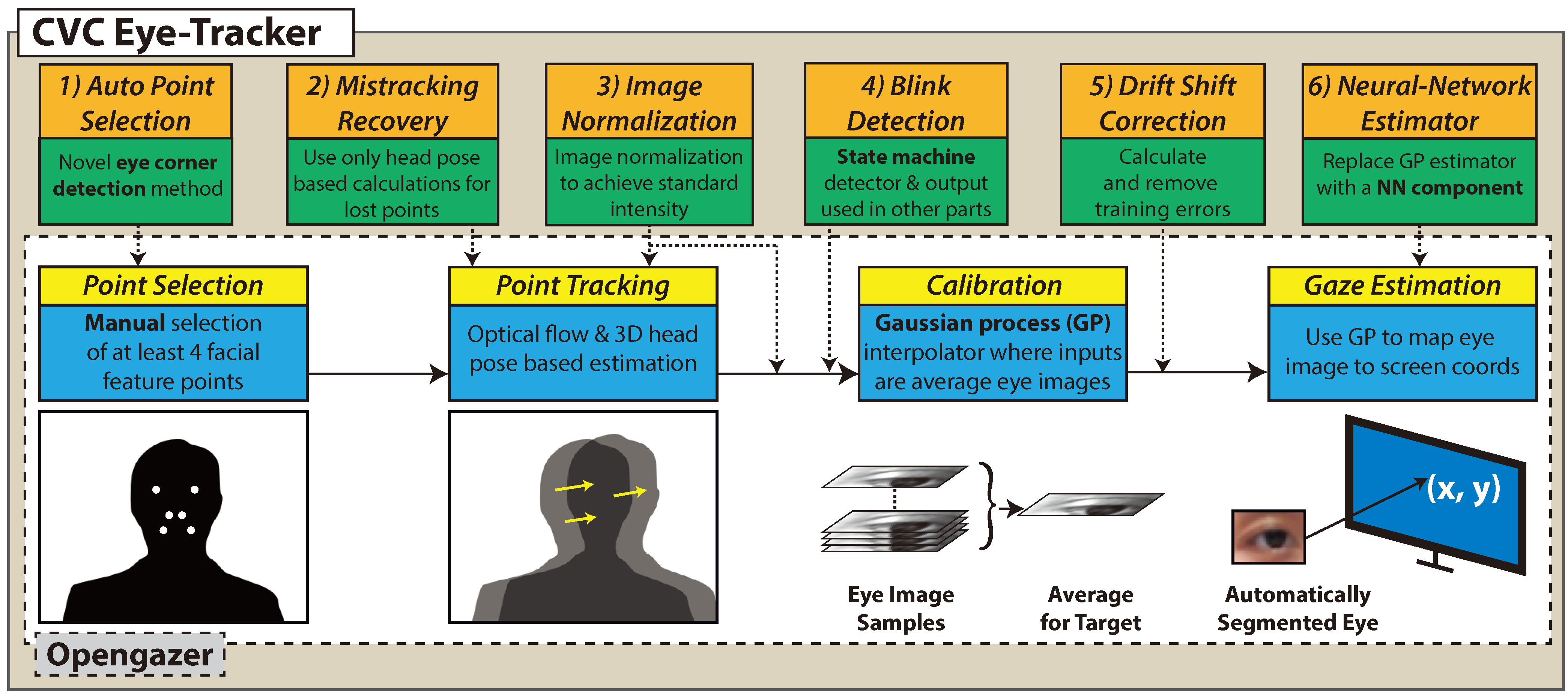
One of the differences of our work from the appearance based methods mentioned above, is that it is a fully automatic system. The auto facial point selection mechanism initializes the system, and the rest of the application does not require much user input. Moreover, the work on the point tracking and image normalization handles the problems such as illumination change. The training error correction improves the estimations especially for targets near the screen corners. These contributions can be seen in Figure 1.
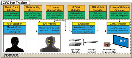
Figure 1.
The pipeline of the eye-tracker and our contributions on top of the base code.
The Eye Tribe and NUIA eyeCharm devices provide cheap alternatives, however they require extra hardware and are not suitable for mobile environments. One of our aims is to solve the eye-tracking problem with software only, or without resorting to special hardware (i.e. software installed on a common device connected to a camera). The Raspberry Pi tracker is a prototype for this kind of eye-trackers. Lastly, the other open source solutions are either infrared based or provide lower accuracies compared to our system.
Method
The components of the software can be seen in Figure 1. The original system requires at least 4 facial feature points chosen manually on subject’s face and it employs a combination of optical flow (OF) and 3D head pose based estimation for tracking them. The image region containing one of the eyes is extracted and used in calibration and testing. In calibration, the subject is asked to look at several target locations on the display while image samples are taken and for each target, an average eye image is calculated to be used as input to train a Gaussian process (GP) estimator. This estimator component maps the input images to display coordinates during testing.
Our first contribution is a programmatic point selection mechanism to automate this task. Then we propose several improvements in the tracking component, and we implement image intensity normalization algorithms during and after tracking. We finish the work on the blink detector to use these detections in other components. In calibration, we propose a procedure to assess and eliminate the training error. For the gaze estimation component, we try to employ a neural network method (Holland & Komogortsev, 2012). In the following subsections, we give the details of these contributions and talk about their effects on system performance in the discussion section.
Point Selection
Our contribution in the automation of the point selection mechanism aims at removing the errors due to operation mistakes. Moreover, it provides a standardized technique which increases the system’s robustness. It employs a combination of Haar cascade detectors (Castrillón-Santana, 2013; Hameed, 2014), geometrical heuristics and a novel eye-corner detection technique. First, a cascade is used to detect the region containing both eyes and then the novel method detects the outer eye-corner points (Figure 2(a)). Here, the proposed method extracts all corner points inside the ROI using Harris detector, and calculates the average corner coordinates in the left and right half of the region. These two points are considered as approximate eye centers and the outer corner points are chosen on the line that passes through them. As we only search a point around the eye corner that is stable enough, we do not make more complex calculations and we simply choose the eye corner points at a predefined distance (1/3 of the distance between two centers) away from the center point approximates.
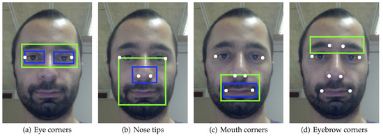
Figure 2.
Sequence of facial feature point selection 3.
After the eye corners are selected, we search the nose in a square region below them. When the Haar cascade returns a valid detection—as in the inner rectangle in Figure 2(b)—, the two nasal points are selected at fixed locations inside this area. The algorithm continues in a similar way for the mouth and eyebrow feature points.
Point Tracking
The point tracking component of the original system uses a combination of optical flow (OF) and 3D head pose based estimation. Optical flow calculations are done between the current camera image and the previous image. This methodology results in the accumulation of small tracking errors and causes the feature points to deviate vastly from their original positions after blinking, for instance. In order to make our eye-tracker more robust to these problems, we modified the tracking component so that OF is only calculated against the initial image saved while choosing the feature points. Moreover, if we still lose track of any point, we directly use the estimate calculated using the 3D head pose and correctly tracked points’ locations.
Image Normalization
During eye-tracker usage, the ambient light may change depending on the sun or other external light sources. Particularly, the computer display itself also acts as a source of frontal illumination, which contributes to a modification of the shades and shadows on the face as images of different intensities are shown in the screen. As the gaze estimation component of our eye-tracker uses intensity images for training and testing, the change in the light level is reflected in the increased error rates of the system.
Normalization Techniques. In order to tackle the varying lighting conditions, we incorporate two image normalization techniques to standardize the intensities over time (Gonzalez & Woods, 2008):
1. Standard pixel intensity mean and variance: In this technique, we first calculate the mean (µorig) and the standard deviation (σorig) of the original image (Iorig) pixels. In the next step, the scale factor (S) is calculated as:
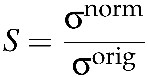 (1)
where σnorm is the desired standard deviation of intensity for the normalized image (Inorm). Finally, the normalized image pixels are calculated with the formula:
(1)
where σnorm is the desired standard deviation of intensity for the normalized image (Inorm). Finally, the normalized image pixels are calculated with the formula:
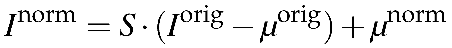 (2)
Here, the equation first scales the image pixels to have the desired standard deviation, then shifts the mean intensity to the desired value.
(2)
Here, the equation first scales the image pixels to have the desired standard deviation, then shifts the mean intensity to the desired value.
(1)
(2)
2. Standard minimum and maximum intensity: The second method aims at normalizing the images so that the minimum and maximum intensity values are the same among all the images.
We start by calculating the minimum (minorig) and maximum (maxorig) pixel intensities in the original image. Then, the scale factor is calculated as:
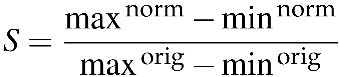 (3)
which is basically the ratio of pixel intensity interval between the desired normalized image and original image. Lastly, the normalized image pixels are calculated as:
(3)
which is basically the ratio of pixel intensity interval between the desired normalized image and original image. Lastly, the normalized image pixels are calculated as:
 (4)
where the image pixels are mapped from range [minorig, maxorig] to [minnorm, maxnorm].
(4)
where the image pixels are mapped from range [minorig, maxorig] to [minnorm, maxnorm].
(3)
(4)
Variations in Usage. Having these two normalization techniques at hand, we continue by incorporating them in the eye-tracker. Normalization takes into account the distribution of gray levels for a given region. In our particular context, this can be applied in a pyramidal approach to: 1) the region containing the eye, 2) the region containing the face, or 3) the whole image. Since the statistics of each region are different, normalization is expected to provide different results depending on the region of application. In addition, normalizing in different regions has an impact in a number of system modules as explained next:
- Eye-region normalization: Only the extracted eye regions are used for the normalization. By applying normalization to the eye-regions we guarantee that the gaze estimation component always receives images with similar intensity distributions.
- Face-region normalization: Normalization parameters are derived and applied to the face region. We make use of the facial feature points’ positions for a fast region segmentation. The bounding box coordinates for these points are calculated and the box is expanded by 80% horizontally and 100% vertically so that the whole face is contained. By normalizing within the face bounding box we aim at improving point tracking by removing the effects of intensity variations.
- Whole-image normalization: By using the whole image, we adapt the normalization to the average light conditions. However, variations in the background can affect the final result. Potentially, changes in the frontal illumination provided by the display can affect stability of the facial feature points detection.
- Combined normalization: Lastly, we apply the eye-region normalization on top of the face-region or whole-image normalizations. By combining both methodologies, we expect to address both the tracking problems and the problems caused by not normalized eye-region images.
Blink Detection
The blink detector is an unfinished component of Opengazer and we continue with analyzing it and making the necessary modifications to get it running. We believe that blinks have an effect on performance and by skipping them during training, we can remove the errors they introduce.
The blink detector is designed as a state machine with initial, blinking and double blinking states. The system switches between these, depending on the differences in eye images that are extracted as described in the previous section. These differences are calculated as the L2 norm between the eye images in consecutive frames. When the difference threshold for switching states is exceeded during several frames, the state is switched to the next state and a blink is detected.
We built on this structure and completed the rules for the state switching mechanism. Moreover, we added a state reset rule that resets the system to the initial state whenever the threshold criteria is not met at a certain frame.
Calibration
The original system uses all the images acquired during the calibration step. We propose a modification in the calibration part which uses our blink detector so that the images acquired during blinks are no longer included in the calibration procedure. This is crucial because these frames can alter the average eye images calculated during calibration and therefore are reflected as noise in the calibration procedure. However; as these frames are no longer available for calibration, we have to increase the time each target point is displayed on the screen in order to provide the system with enough samples during calibration.
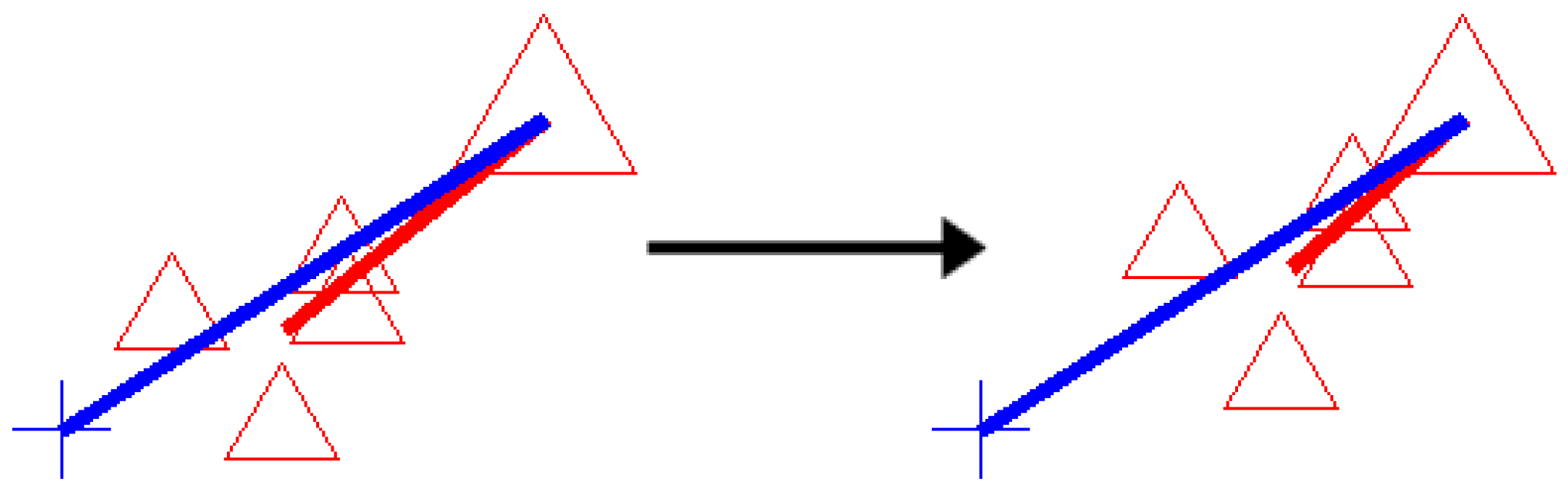
Another improvement that we propose is the correction of calibration errors as illustrated in Figure 3.

Figure 3.
The drift correction moves the estimates (small signs) towards the actual target (larger signs). The training error direction (blue line) and testing error direction (red line) show the correlation.
Here, red triangles on the left side correspond to a target point displayed on the screen and the corresponding gaze estimations of our system, one for each camera frame. The larger symbol denotes the actual target, whereas the smaller ones are the estimates. The shorter line connects the average estimation and the target location. Therefore, the length and direction of this line gives us the magnitude and direction of average testing error. Apart from these symbols, the longer line that starts from the target denotes the direction of the calibration error. However, it should be noted that in order to easily observe the direction, the magnitude of the calibration error is increased by a factor of 5. In this figure, we can see the correlation between the calibration error and average testing error, therefore we propose a correction method. The final effect of this technique can be seen on the right side, where the estimates are moved closer to the actual target point.
To calculate the calibration errors, we store the grayscale images which are used to calculate the average eye images during calibration. Therefore, we save several images corresponding to different frames for each target point. After calibration is finished, the gaze estimations for these images are calculated to obtain the average gaze estimation for each target. The difference between these and the actual target locations gives the calibration error.
After the calibration errors are calculated, we continue with correcting these errors during testing. We employ two multivariate interpolators (Wang, Moin, & Iaccarino, 2010; MIR, 2014) which receive the average gaze estimations for each target point as inputs and are trained to output the actual target x and y coordinates they belong to. The parameters that we chose for the interpolators are: approximation space dimension ndim = 2, Taylor order parameter N = 6, polynomial exactness parameter P = 1 and safety factor sa f ety = 50. After the interpolator is trained, we use it during testing to remove the effects of calibration errors. We pass the currently calculated gaze estimate to the trained interpolators and use the x and y outputs as the corrected gaze point estimation.
Gaze Estimation
Originally, gaze estimates are calculated using the image of only one eye. We propose to use both of the extracted eye images to calculate two estimates. Then, we combine these estimations by averaging.
We also consider the case where the GP interpolator is completely substituted in order to see if other approaches can perform better in this particular setup. Neural network (NN) methods constitute a popular alternative for this purpose. There exist recent implementations of this technique (Holland & Komogortsev, 2012). In the aforementioned work, an eyetracker using NNs to map the eye image to gaze point coordinates is implemented and is made available (Komogortsev, 2014).
We incorporated the NN method in our system by making use of the Fast Artificial Neural Network (FANN) library (Nissen, 2003) and created a similar network structure, and a similar input-output system as the original work. Our neural network had 2 levels where the first level contained 128 nodes (1 for each pixel of 16 × 8 eye image) and the second level contained 2 nodes (one each for x and y coordinates). We scaled the pixel intensities to the interval [0, 1] because of the chosen sigmoid activation function.
Experimental Setup
In this section, we give the details of the experimental setup we created to test the performance of our application. Variations in the setup are introduced to create separate experiments which allow us to see how the system performs in different conditions. Figure 4 shows how the components of the experimental setup are placed in the environment.
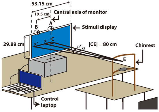
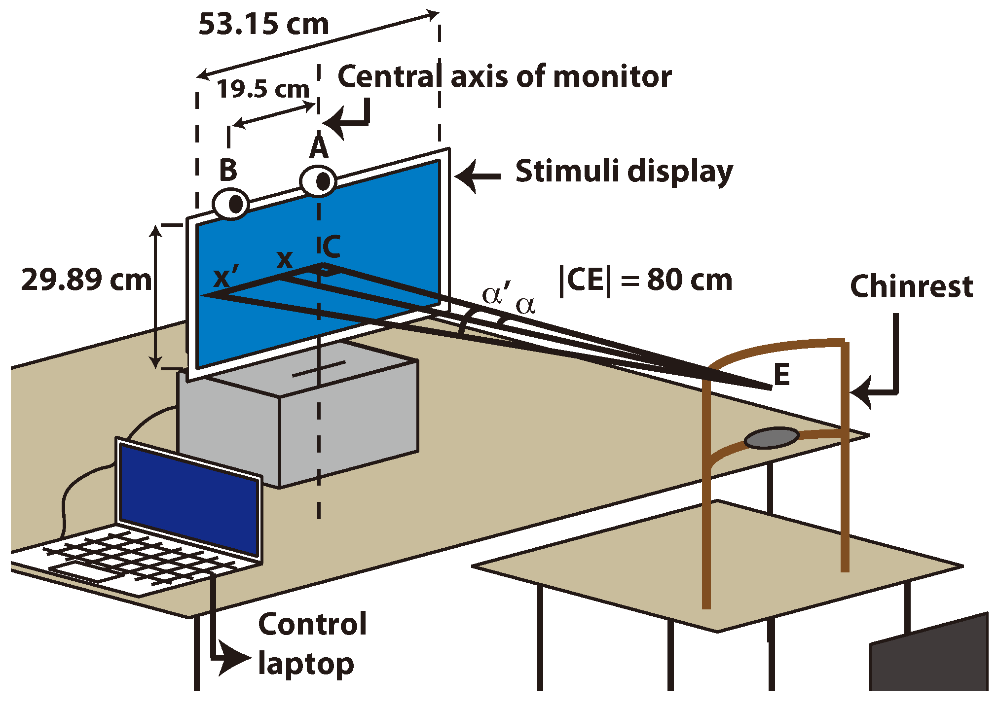
Figure 4.
Placement of the components in the experimental setup and the geometry involved in error calculation.
The stimuli display faces the subject and it is raised by a support which enables the subject to face the center of the display directly. The camera is placed at the top of this display at the center (A), and it has an alternative location which is 19.5 cm towards the left from the central location (B). An optional chinrest is placed at the specific distance of 80 cm away from the display, acting as a stabilizing factor for one of the experiments.
By introducing variations in this placement, we achieve several setups for several experiments which test different aspects of the system. These setups are:
- Standard setup: Only the optional chinrest is removed from the setup shown in Figure 4. Subject’s face is 80 cm away from the display. The whole screen is used to display the 15 target points one by one.
- Extreme camera placement setup: This setup is similar to the previous one. The only difference is that the camera is placed at its alternative location which is 19.5 cm shifted towards the left. The purpose of this setup is to test how the position of the camera affects the results.
- Chinrest setup: A setup similar to the first one. The only difference is that the chinrest is employed. This experiment is aimed at testing the effects of head pose stability in the performance.
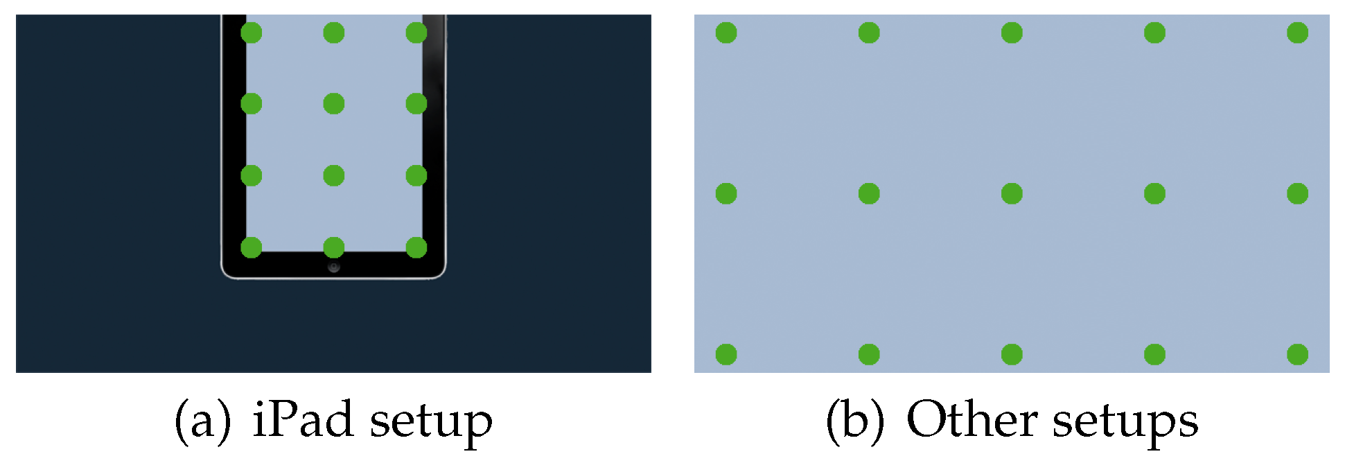
- iPad setup: This setup is used to test the performance of our system simulating the layout of an iPad on the stimuli display. This background image contains an iPad image where the iPad screen corresponds to the active area in the experiment and is shown in a different color (see Figure 5(a)). The distance of the subject is decreased to 40 cm, in order to simulate the use-case of an actual iPad. The camera stays in the central position; and it is tilted down as seen necessary in order to center the subject’s face in the camera image.
 Figure 5. Target positions on the display for different setups.
We also analyze the effect of different camera resolutions in these setups. This is done in an offline manner by resizing the original 1280 × 720 image to 640 × 480.
The error in degrees is calculated with the formula:
where, x is the target, x′ is the estimate, C is the display center and E is the face center point. The variables DxC, DEC and so on denote the distances between the specified points. They are converted from pixel values to cm using the dimensions and resolution of the display.
Error = |arctan(DxC/DEC) − arctan(Dx′C/DEC)|
For the evaluation of normalization techniques, the videos recorded for the standard setup are processed again with one of the normalization techniques incorporated into the eye-tracker at a time.
Results
In this section, we present the results which show the effects of the proposed changes on the performance. To achieve this, we reflect our changes on the original Opengazer code one by one and compare the results for all four experiments. We compare 6 different versions of the system which denote its certain phases:
- [ORIG] Original Opengazer application + automatic point selection
- [2-EYE] Previous case + average estimate of 2 eyes
- [TRACK] Previous case + tracking changes
- [BLINK] Previous case + excluding blinks during calibration
- [CORR] Previous case + training error correction
- [NN] Previous case + neural network estimator
In all versions, the facial feature points are selected automatically by the method described in previous sections and gaze is not estimated during blinks. For each experiment, average horizontal and vertical errors for all subjects and all frames are given in degrees and the standard deviation is supplied in parentheses.
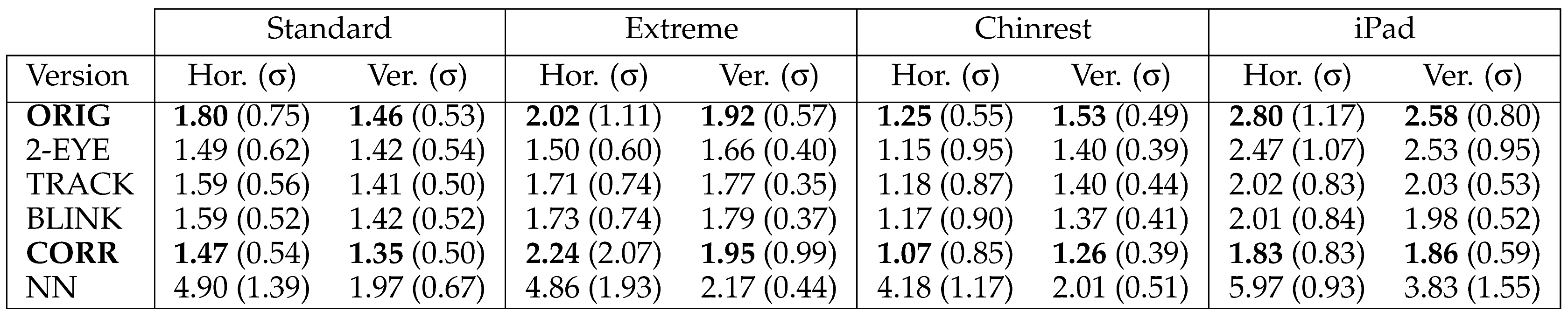
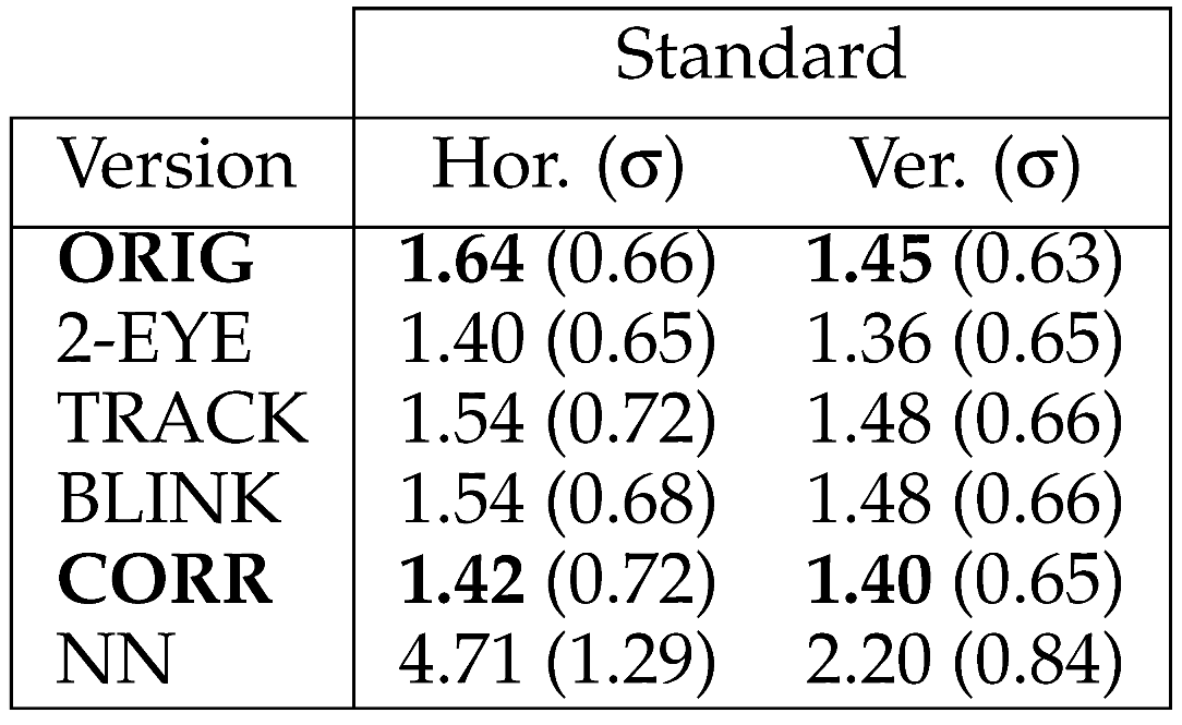
Table 1 shows the progressive results of our eyetracker’s performance for different versions of the system. Each result column denotes the horizontal or vertical errors for a different experimental setup. Moving from top to bottom in each column, the effects of our changes can be seen for a single error measure of an experimental setup. Along each row, the comparison of errors for different setups can be observed. Table 2 shows the performance values of the system in the standard setup with the lower resolution camera. These results can be compared to the high resolution camera’s results as seen in Table 1 to see how the camera resolution affects the errors in the standard setup. The original application’s results (ORIG) and our final version’s results (CORR) are shown in boldface to enable fast comparison.

Table 1.
Errors in degrees with 1280 × 720 camera resolution for all setups.
Table 2.
Standard setup errors in degrees with 640 × 480 resolution.
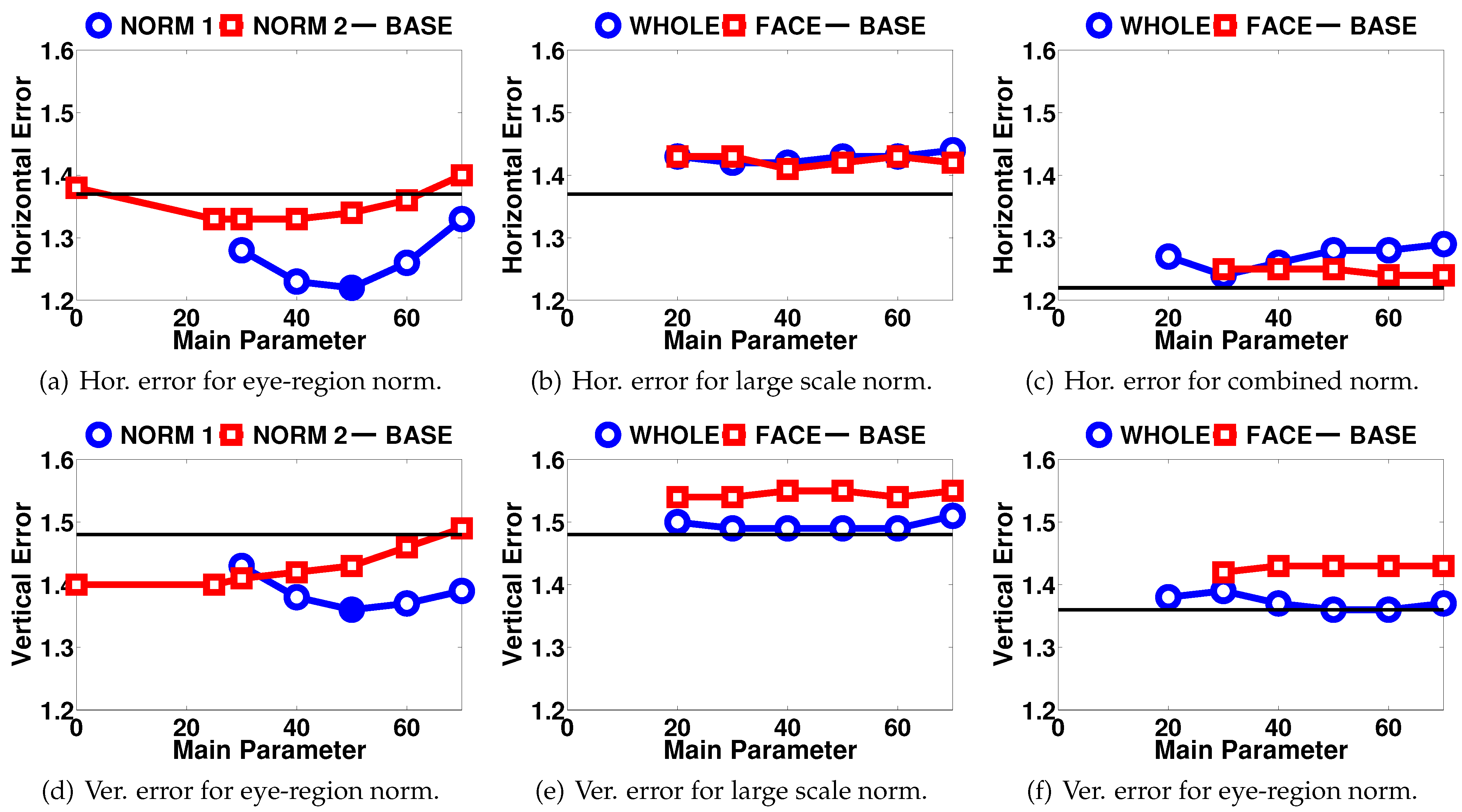
As for the normalization contributions, the results are grouped in Figure 6. Figure 6(a) and 6(d) show the results for the two techniques applied on the eye images. The black baseline shows the best results of the system without any normalization (1.37° horizontal, 1.48° vertical errors). For the standard pixel intensity mean and variance normalization (NORM 1), the standard intensity mean parameter is fixed to 127 and several values are evaluated as the standard deviation parameter (main parameter). This choice was made because when the standard deviation parameter is selected, the mean parameter does not affect the gaze estimations unless it results in the trimming of pixel intensities (mapping to intensities outside the range [0, 255]). In the case of standard minimum and maximum intensity normalization (NORM 2), the minimum intensity parameter is considered the main parameter and the maximum intensity is set to: maxnorm = 255 − minnorm.
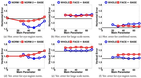
Figure 6.
Errors in degrees for eye image normalization techniques. (a) and (d) show errors for eye-region normalization. In (b) and (e), the errors for only face-region and whole-image normalization methods are shown. These methods apply the first normalization technique in the corresponding image areas. Lastly, (c) and (f) show the results where the eye-region normalization is applied on top of either the whole-image or the face-region normalization. The black straight lines show the baseline accuracy for comparison. In (a), (b), (d) and (e), this corresponds to the error rate without any normalization. In (c) and (f), it denotes the best results so far, which belong to the eye-region normalization using technique 1 (filled data points in (a) and (d)).
In Figure 6(b) and 6(e), the second set of normalization results are shown. Here, the better performing NORM 1 technique is applied to the whole camera image (WHOLE) or the face-region (FACE) and the results are given.
Lastly, Figure 6(c) and 6(f) show the results when the eye-region normalization is combined with wholeimage or face-region normalizations. As the eye-region normalization is independent of the others, the parameters for this step are fixed to the best performing values (µnorm = 127, σnorm = 50) and the black baseline shows the best results achieved with only eye normalization (1.22° horizontal, 1.36° vertical errors).
Discussion
Considering the 1.47° horizontal and 1.35° vertical errors of the final system in the standard experimental setup, we conclude that we have improved the original system by 18% horizontally and 8% vertically. As seen in Table 2, the performance difference in the same experiment done with VGA cameras (13% horizontally, 3% vertically) is comparably lower than the first case, which shows us that our contributions in this work exhibit more robust performance with the increased image quality. From another aspect, it means that better cameras will favor the methods we proposed in terms of robustness.
One interesting aspect of these results is that with the increased camera resolution, the original application shows a worse performance. We believe this is caused by the optical flow algorithm used in the tracking component. The increased detail in the images affect the tracking and the position of the tracked point may vary more compared to the lower resolution image. This, combined with the accumulated tracking error of the original application, result in a higher error rate. However, it is seen that the final version of our eye-tracker (CORR) recovers most of this error.
From the extreme camera placement setup results seen in Table 1, we see that shifting the camera from the top center of the display decreased the performance by 52% horizontally and 44% vertically. Here, the performance loss is mainly caused by the point tracking component. From such a camera angle, the farther eye corner point may be positioned on the face boundary, making it hard to detect and track. When we compare the errors before and after the error correction is applied (BLINK and CORR), we see that this change introduced a great amount of error for this case. We can say that the unreliable tracking also hinders the error correction component, because the correction relies on the calibration being as good as possible. In order to tackle these problems, a 3D model based face tracking algorithm may be employed.
In the 3rd experimental setup, we show that the chinrest improves the performance by 27% horizontally compared to the standard setup. This setup proves to be more reliable for experimental purposes.
The results for the iPad setup may be deceiving, because here actually the errors in pixels are lower; however, as the distance of the subject is used in the calculation of errors in degrees, the angular errors are higher.
Each 1° error in other setups corresponds to around twice as many pixels on the screen compared to a 1° error in the iPad setup. Using this rule of thumb, we can see that the iPad case results in lower error rate in pixels compared to even the chinrest setup.
One of the major problems with the original system lies in the tracking component. As tracking is handled by means of optical flow (OF) calculations between subsequent frames, the tracking errors are accumulated and the facial feature points end up far away from their original locations. To tackle this problem, we proposed to change this calculation to compare the last camera frame with the initial frame which was saved during facial feature point selection. Comparing the 2-EYE and TRACK results in Table 1, we see that the tracking changes increased the system’s accuracy in the iPad setup. However, in the first two setups we have just the opposite results. This is probably because when using both of the eyes for gaze estimation, the tracking problems with the second eye have a larger effect on the averaged gaze estimation.
We observe that excluding the blink frames from the calibration process (application version labeled BLINK) does not have a perceivable effect on the performance. We argue that the averaging step in the calibration procedure already takes care of the outlier images. The neural network estimator does not provide an improvement over the Gaussian process estimator and performs similar to its reported accuracy (4.42°). We believe this is due to eye images extracted by our system. Currently the feature point selection and tracking mechanism allows small shifts in point locations and therefore the extracted eye images vary among samples. The GP estimator resolves this issue during the image averaging step; however, the NN estimator may have problems when the images vary a little in the testing phase. In order to resolve this problem, a detection algorithm with a higher accuracy may be used to better estimate the eye locations.
Analyzing the eye image normalization results as seen in Figure 6(a) and 6(d), we see that both approaches improve the results. For the first normalization technique, the parameter value giving the best results is σnorm = 50, which decreases the errors by 11% horizontally and 8% vertically. We can say that the eye image normalization does just what the Gaussian process estimator needs and helps compare eye images from different time periods in a more accurate way. The results for the second normalization method lag behind especially in the horizontal direction.
Figure 6(b) and 6(e) show the results for intensity normalization in the large scale, either applied to the whole camera image or around the face region. Here, we see that large scale normalization applied on top of eye image normalization does not improve the results at all. Our expectations for the face normalization to perform better than whole image normalization are not verified, either. We observe that the face normalization performs especially worse in vertical direction.
Conclusion
Our contribution provides significant improvement in a number of modules for the state of the art of low cost eye-trackers using natural light. Our automatic point selection technique enabled us create an easy to use application, removing errors caused by wrong operation. The experiments showed that the final system is more reliable in a variety of scenarios. The blink detection component is mostly aimed at preparing the eye-tracker to real world scenarios where the incorrect estimations during blinks should be separated from meaningful estimates. The proposed error correction algorithm helped the system better estimate gazes around the borders of the monitor. Lastly, the eye image normalization technique improved the performance of the system and made the system more robust to lighting conditions slightly changing in time. The final code can be downloaded from the project page (Ferhat & Vilariño, 2014a). Apart from these experimental performance assessments, our work resulted in additional valuable outputs:
- A Portable Eye-Tracker: We installed our system on a Raspberry Pi and achieved a cheap (€70) alternative to commercial eye-trackers. This system can be used as a separate input device to calculate and send the gaze point to the main computer. For experimental purposes, the necessary results analysis tools are also included in the device. The device has the same final error rates as in the experimental results (1.42° horizontally and 1.40° vertically for 640 × 480 resolution) and has a 3Hz update rate. By optimizing the code and using a faster camera, we expect to increase the refresh rate of the system. The SD card image for the resulting system can be downloaded from the project page (Ferhat & Vilariño, 2014a).
- An Eye-Tracking Video Dataset: The videos recorded during the experiments are gathered in a dataset of 12 subjects and 4 different experiment cases (Ferhat & Vilariño, 2014b).
- The annotations for the videos denote on which frame the training and testing phases start and the ground truth gaze points at a given frame.
Funding
This work was supported in part by the Spanish Gov. grants MICINN TIN2009-10435 and Consolider 2010 MIPRCV, and the UAB grants.
References
- Baluja, S., and D. Pomerleau. 1993. Non-intrusive gaze tracking using artificial neural networks. In NIPS. Edited by J. D. Cowan, G. Tesauro and J. Alspector. Morgan Kaufmann: pp. 753–760. [Google Scholar]
- Castrillón-Santana, M. 2013. Modesto Castrillón-Santana. Retrieved from http://mozart.dis.ulpgc.es/Gias/modesto.html.
- 2014. The Eye Tribe. Retrieved from http://theeyetribe.com/.
- Ferhat, O., and F. Vilariño. 2014a. CVC Eye-tracker project page. Retrieved from http://mv.cvc.uab.es/projects/eye-tracker.
- Ferhat, O., and F. Vilariño. 2014b. CVC Eye-Tracking DB. Retrieved from http://mv.cvc.uab.es/projects/eye-tracker/cvceyetrackerdb.
- Gonzalez, R. C., and R. E. Woods. 2008. Digital image processing. Upper Saddle River, N.J.: Prentice Hall. Retrieved from http://www.worldcat.org/search?qt=worldcat_org_all&q=013505267X.
- Hameed, S. 2014. Haar cascade for eyes. Retrieved from http://www-personal.umich.edu/%7Eshameem.
- Hansen, D. W., J. P. Hansen, M. Nielsen, A. S. Johansen, and M. B. Stegmann. 2002. Eye typing using Markov and Active Appearance Models. In WACV. IEEE Computer Society: pp. 132–136. [Google Scholar]
- Hansen, D. W., and Q. Ji. 2010. In the eye of the beholder: A survey of models for eyes and gaze. IEEE Trans. Pattern Anal. Mach. Intell. 32, 3: 478–500. [Google Scholar] [PubMed]
- Holland, C., and O. V. Komogortsev. 2012. Eye tracking on unmodified common tablets: challenges and solutions. In ETRA. Edited by C. H. Morimoto, H. O. Istance, S. N. Spencer, J. B. Mulligan and P. Qvarfordt. ACM: pp. 277–280. [Google Scholar]
- 2014. ITU Gaze Tracker. Retrieved from http://www.gazegroup.org/downloads/23-gazetracker.
- Komogortsev, O. V. 2014. Identifying fixations and saccades in eye tracking protocols. Retrieved from http://cs.txstate.edu/%7Eok11/nnet.html.
- Lu, F., T. Okabe, Y. Sugano, and Y. Sato. 2011. A head pose-free approach for appearance-based gaze estimation. In Proceedings of the British Machine Vision Conference. BMVA Press: pp. 126.1–126.11. [Google Scholar] [CrossRef]
- Lu, F., Y. Sugano, T. Okabe, and Y. Sato. 2011. Inferring human gaze from appearance via adaptive linear regression. In Iccv. Edited by D. N. Metaxas, L. Quan, A. Sanfeliu and L. J. V. Gool. IEEE: pp. 153–160. [Google Scholar]
- 2014. MIR. Retrieved from http://sourceforge.net/projects/mvinterp.
- Nissen, S. 2003. Implementation of a Fast Artificial Neural Network Library (FANN). Report, Department of Computer Science University of Copenhagen (DIKU) 31. [Google Scholar]
- 2014. NUIA eyeCharm. Retrieved from https://www.kickstarter.com/projects/4tiitoo/nuia-eyecharm-kinect-to-eye-tracking.
- Sugano, Y., Y. Matsushita, and Y. Sato. 2013. Appearancebased gaze estimation using visual saliency. IEEE Trans. Pattern Anal. Mach. Intell. 35, 2: 329–341. [Google Scholar] [CrossRef] [PubMed]
- Sugano, Y., Y. Matsushita, Y. Sato, and H. Koike. 2008. An incremental learning method for unconstrained gaze estimation. In ECCV (3). pp. 656–667. [Google Scholar]
- Valenti, R., N. Sebe, and T. Gevers. 2012. Combining head pose and eye location information for gaze estimation. IEEE Transactions on Image Processing 21, 2: 802–815. [Google Scholar] [CrossRef] [PubMed]
- Wang, Q., P. Moin, and G. Iaccarino. 2010. A high order multivariate approximation scheme for scattered data sets. Journal of Computational Physics 229, 18: 6343–6361. [Google Scholar] [CrossRef]
- Xu, L.-Q., D. Machin, and P. Sheppard. 1998. A novel approach to real-time non-intrusive gaze finding. In BMVC. Edited by J. N. Carter and M. S. Nixon. British Machine Vision Association. [Google Scholar]
- Zielinski, P. 2013. Opengazer: open-source gaze tracker for ordinary webcams (software). Retrieved from http://www.inference.phy.cam.ac.uk/opengazer/.

Copyright © 2014. This article is licensed under a Creative Commons Attribution 4.0 International License.