Additive mixture model to explain eye fixation distribution
The most common technique to create density maps is to make convolution between the fixations map and a Parzen kernel (here for example a Gaussian kernel adjusted with the fovea size). It is a non-parametric method which is not useful to extract the clustering structure of the data. So we prefer a parametric modeling using an additive mixture model. Moreover, in the case of noisy data or of lack of robust data, we complete this model with a “random mode” to extract a part of the noisy structure in the data. Therefore, in this section we present the use of an additive mixture Gaussian method to model the spatial distribution of eye-fixations, first without the “random mode”, and secondly with the “random noise”.
This approach is commonly used to estimate the spatial gaze density function. This method is “imagedependant” because its interpretation is directly linked to the objects which compose the scene. The Gaussian additive mixture model is implemented with the “Expectation-Maximisation” algorithm (
Dempster, Laird & Rubin, 1977) as a statistical tool for density estimation. The density function
f(x) of a random uni or multivariate variable
x is estimated by an additive mixture of
K Gaussian modes according to the following equation:
with
K the a priori number of Gaussian modes,
pk the weight of each mode (
p1+…pK = 1),
ϕ(x; θk) the Gaussian density of the k
th mode and
θkits parameter (mean and covariance matrix).
The number of modes (K) is a priori unknown and must be chosen. The selection model assesses the fitting quality (higher value for K) and the robustness without overtraining (lower value for K). A classical approach is to use an information criterion which balances the likelihood of the model with its complexity (
Hastie, Tibshirani & Friedman, 2001). Among the different available criteria, the Bayesian Information Criterion (BIC) (
Schwarz, 1978) is preferred in a density estimation context (
Keribin, 2000). A range of possible values of K is chosen depending on the complexity of the visual scene. For each value of K in this interval, the optimal parameters
(pk, θk, k = 1...K) of the mixture are found at the convergence of the Expectation-Maximization algorithm (“EM” algorithm,). From all these sets of parameters, the “best” model is selected: it minimizes the BIC criterion:
with
L the maximum log-likelihood of the estimated model at the “EM” convergence, ν the number of free parameters and
n, the number of observed data.
Figure 1 illustrates this model on eye fixations dataset when people freely gaze at this visual scene during 8 seconds. The range for the candidate values for
K is between one and eight (this value is large enough according to the number of objects in the scene).
In this example the BIC criterion reaches its optimum for
K=6 when
K varies from one to eight. The best model has thus six Gaussian modes (
Figure 1a).
Figure 1b shows the localization of these modes. Each mode is illustrated by its position (mean) and its spreading at one standard deviation (ellipse). These modes describe the spatial areas which are fixated during the scene exploration, i.e. the probability for each area to be gazed at.
Figure 1c illustrates the resulting spatial density function
f(.). Moreover, we can notice that the configuration with seven Gaussian modes can be also a “good” solution: the values for the BIC criterion are very close between these two configurations (
BIC = -289.50 with
K = 6,
BIC = 289.12 with
K = 7). After that the BIC value increases (
BIC = -280.02).
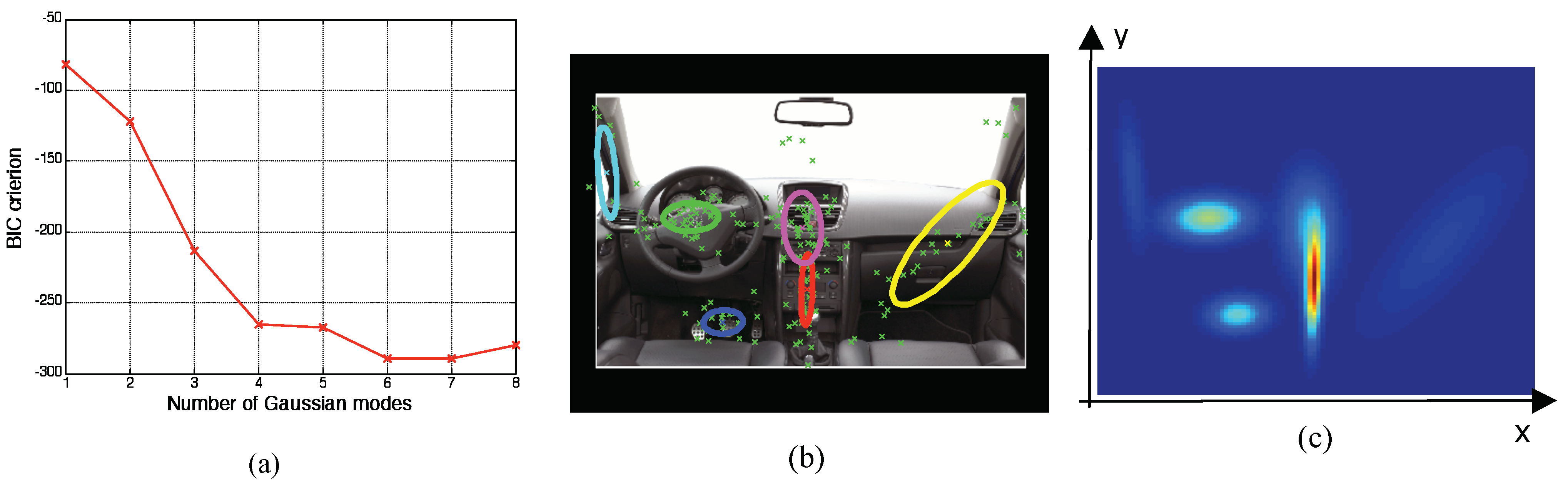
This example illustrates also one common difficulty when using the classical “EM” algorithm faced with noisy data. If the latent data clustering is not very strong, some Gaussian modes can be extracted or not depending on the random initial conditions. That it is the case with the vertical Gaussian mode close to the left side of the image; its extraction depends on the initial conditions. To cope with such situations, we add a supplementary mode in the model: a uniform density. The experimental observations which are not close to latent clusters get contributions to this mode: it is the “noise” mode. The equation of the complete model is then:
with K the a priori number of Gaussian modes, p
k the weight of each Gaussian mode,
pu the weight of the uniform mode (
p1 + …pK + pu=1),
ϕ(x; θk) the Gaussian density of the k
th mode and
U(x) the uniform constant density such as
![Jemr 03 00010 i005]()
. The “EM” algorithm is adapted to this model in order to estimate also the contribution
pu. So the model selection concerns the two previous ones, with or without the uniform mode. For the same data, the results are illustrated at figure 2. The minimum value of the BIC criterion is -295.60. This value is reached for the model with four Gaussian modes and the uniform mode.
The contributions of each mode are presented in
Table 1. We notice the contribution
pu is significant compared to the contributions for the Gaussian modes. This uniform mode explains scattered data. Here there are scattered eye fixations which are not localized on specific areas (around here 17% of the whole fixations), i.e “ambient” eye fixations which are very sensitive to inter-individual variability.
This approach, combining Gaussian mixture and the “EM” algorithm, is common to estimate density functions. Depending on their position and deviation, the modes can be interpreted according to the objects in the scene. Here, the three modes in the left side among the four modes in this scene are related to objects: the steering wheel, the pedals, and the central desk. These objects are very important for the interpretation of the scene. But this approach does not reveal for a given task, if some modes are induced by a similar factor, or if a factor has similar effects on visual scenes which have not similar semantic properties.
Nevertheless, we keep this statistical model as a general framework to set-up the new model in which the modes are not necessarily Gaussian. They must represent the candidate guiding factors across different visual scenes for the same task and not spatial concentrations of eye fixations for a given visual scene.
According to the previous section, the mixture model can be set depending on the density properties of the experimental data. But it can also be done by a priori hypotheses defining the number and the properties of each mode of the mixture. Then the global contribution of the whole fixations to each mode is estimated. This approach is employed by Vincent et al. (
Vincent et al., 2009) where the eye positions density is modeled with a mixture of elementary a priori defined densities, each density representing a specific factor which might guide the visual attention. Thus, each mode of the additive mixture is defined by a density modeling one candidate factor which might drive the cognitive analysis of the visual task. The common properties of these two models are the additive mixture of the modes and the “EM” algorithm to define their configuration parameters.
These factors describe both low level and high level processes. Each mode is used to assess the contribution of the associated factor. First, it is necessary to identify these candidate factors, in relation to the visual task and then, their statistical density model. Each of these densities is represented by a spatial density map, either from a specific image processing, or from a manual segmentation and or also from statistical hypotheses, depending on the nature of the attention factors. The “EM” algorithm provides stable results if the a priori distributions are not strongly correlated. Each distribution which codes a guiding factor must provide complementary effect on the studied process, the visual attention. At the convergence of the “EM” algorithm, the contributions of each density are estimated, maximizing the likelihood of the final model which is then completely defined.
To summarize, a noticeable characteristic of this method is that the additive model contains a priori density maps, which are chosen depending on the stimuli, the tasks, and the assumptions to be investigated, and which must be previously characterized.
Setting up the a priori distributions composing the model
Five factors are suggested to explain the observed fixation distribution, each one being modeled by one spatial distribution and being considered as one mode of the additive mixture.
First of all, if the eyes are guided by a random process, the distribution will follow a uniform law: each area of the space has the same probability of being gazed at. In the mixture, this map acts as a “trash” map, capturing fixations which are not explained by other assumptions.
The second factor is a process of central gazing (
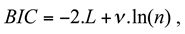
Tatler, 2007): the “on screen” gazing produces a central bias: the eyes preferentially gaze at the center of the screen and tend to return to it regularly, regardless of the content of the image. This is also the initial gaze position and may also be a rest position. A “centrality map” is thus defined, where the central area has a higher probability to be fixed than peripheral ones. The density is determined by a Gaussian function applied to the center of the image. In the original model proposed by Vincent, the mean and the variance covariance matrix will be adjusted during the algorithm as in a usual “EM” algorithm. Here these parameters are fixed because we want to evaluate the contribution of this factor in the central area (see Figure 3).
Indeed, if these parameters are set after learning from the “EM” algorithm, this spatial mode can move or not in another place depending on the visual scene.
The third factor comes from the visual bottom-up saliency. One of the basic principles is that the eyes are attracted towards areas of high contrasts combining different low level visual features on textural luminance and chrominance variances. The bottom-up saliency model proposed by Itti (
Itti & Koch, 2001) is very popular in this domain. In this work, we use a similar algorithm which is developed in our laboratory. It is based on the same general principles as Itti’s, but using a more accurate model at the retina level (
Ho, Guyader & Guérin-Dugué, 2009). This map is considered here as merging low-level visual information to predict the relative attractiveness of spatial areas without “top-down” attention factors (see Figure 4).
The fourth factor is based on an information maximization approach (see Figure 5): it comes from experimental observations (
Renninger, Coughlan & Vergheese, 2005) that the eyes can be spatially positioned in such way to optimize the acquisition of visual information instead of sweep over an area to encode each information. This approach needs to compute from which point of view the details’ perception is maximized, limiting the number of saccadic movements. The edges are then extracted by an edge detector (here the “Sobel” detector).Then a spatial clustering algorithm is used to find the position of the edges barycenters. We use the “Mean Shift” algorithm (
Fukunaga & Hostetler, 1975;
Cheng, 1995). Finally, a Gaussian function, set up with the fovea size, is defined for each cluster and centered on each barycenter. For this factor, the highest probability of gazing at an area is located at the barycenters of the edges and their neighboring areas.
The last factor is a semantic top-down factor: the visual attention is driven by cognitive processes and therefore by the semantic content of the visual scene. Thus, we have to extract the local areas of the scene which contain relevant information regarding the task. To model this factor, we use complementary experiments with the “Bubbles” paradigm using the same visual scenes and the same tasks. Our hypothesis is: the resulting “classification map” obtained by this paradigm gathers the topdown effects in the observed eye fixations density. The constructions of these maps are detailed in the next section (see Figures 6 & 7).
After having estimated the spatial density distribution of each factor and measured the eye-movements, the “EM” algorithm is employed in combination with the additive mixture model to find the best parameters for the model. In our case, these parameters are the relative contribution of each mode (each factor) to the eye fixations density. In the next section, we provide the details of the method to build the semantic map, based on the “Bubbles” paradigm.
Semantic map construction from the “Bubbles” paradigm
Material & Methods
For the top-down factor, we want to extract the relevant parts of the visual scene which should be observed to solve the given task. As far as we know, the “Bubbles” paradigm (
Gosselin & Schyns, 2001) has never been employed to compare semantic information and bottom-up effects on visual attention. We apply it here to select, for a given couple image × task, the visual areas encoding relevant information to solve the judgment task. This paradigm was originally designed to identify facial areas associated with facial expressions recognition (
Humphreys et al., 2006). It consists in watching the scene through a mask, with only a few parts being maintained visible (the “Bubbles”, which are spatially set at random).
Therefore the participants must solve a decision task while gazing the scene through the “Bubbles” mask. This method is relevant when the task resolution requires the capture of local visual information in the scene. The fixation density distribution shows areas which attract the visual attention and the “Bubbles” method identifies the decision areas. Moreover it shows whether the decision is really about local areas or not, and if the judgment task is homogenous or not between participants.
To summarize, this method is efficient when there is a “ground truth” which is related to the correct answers, when the decision is based on local visual areas, and when the decision criteria are stable.
Otherwise, if several “correct answers” exist, if the different visual scenes cannot be discriminated by local areas, or if the decision is subject-dependant, then the algorithm will not be able to extract local areas statistically associated with consensual decisions.
![Jemr 03 00010 i001]()
The “Bubbles” paradigm proposed by Gosselin (
Gosselin & Schyns, 2001) statistically links the subjects’ answers with the areas of the visual scene gazed during a decision task. These local areas are called the “diagnostic areas”.
The stimuli we employ are visually and semantically complex, and the decision activates high-level processes. Moreover, a consensus between participants is necessary in order to extract some stable diagnostic areas: one “right” answer and a “false” one must exist, and this alternative must be homogenous to all the participants.
Therefore, we adapt this paradigm to a paired-wise comparison task, in order to assess the stimuli with a reference (
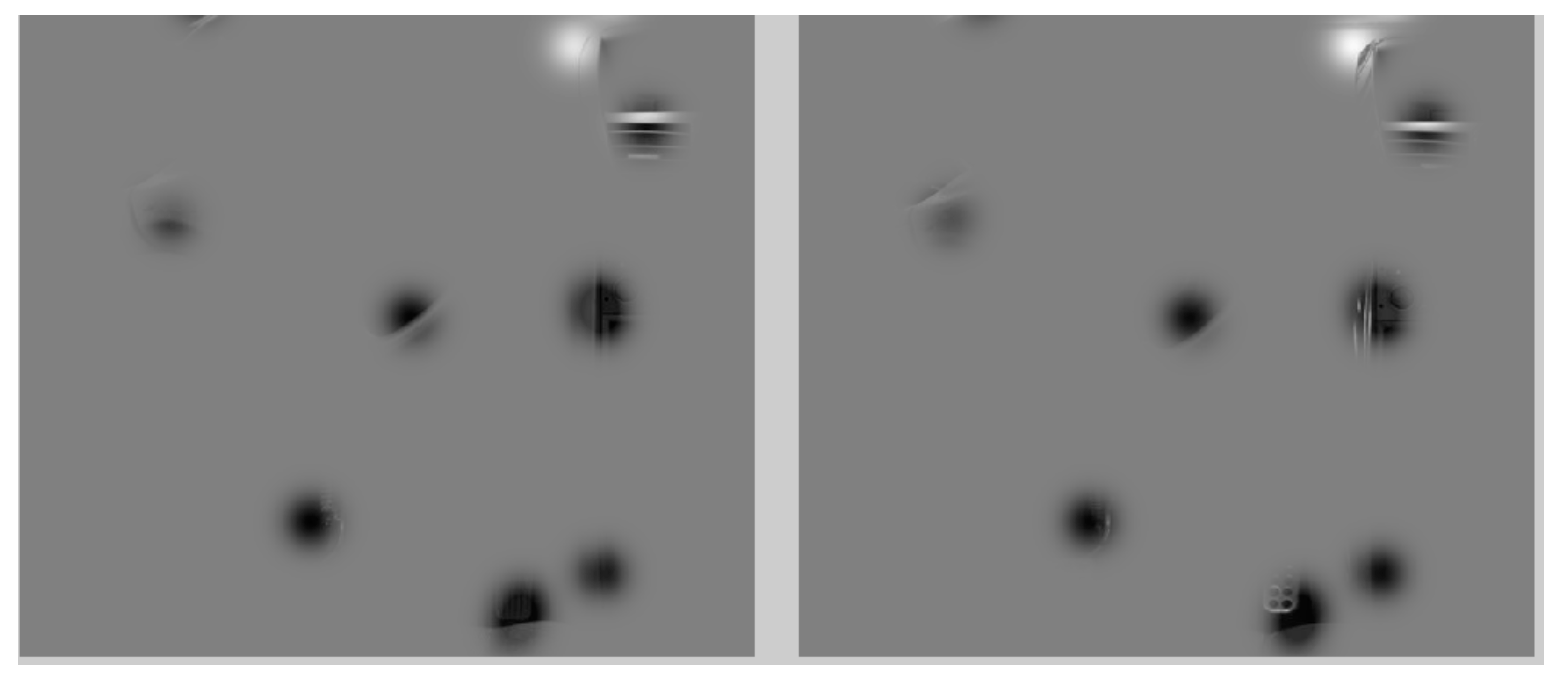
Humphreys et al., 2006). The “Bubbles” are set at random for one image of the pair and the same localizations are set for the second image. See
Figure 7. The decision is taken after the visual inspection of both images of the pair, having a similar masking (left and right sides of the screen): in the pair, one image has the required property, the second, does not. The description of the different properties studied of the car’s cab interiors are described in the next section.
The algorithm adjusts automatically the number of “Bubbles”, to be adapted to the performance of the participants (from 70 up to 80% of correct answers) during the trial and will move towards a setup threshold of correct answers. The surface of each bubble is set such as its radius is one angular degree (fovea). On average (depending on the complexity of the scene), between 10% and 15% of the picture is visible. Finally the algorithm estimates the correlations between the correct answers and the position of the visible areas, and provides a probabilities distribution. This is the probability for a spatial area to be associated to a right answer. In other words, the “Bubbles” paradigm provides a spatial map of right decision making: the classification map.
The experiment was designed with the Stat4Ci (
http://www.mapageweb.umontreal.ca/gosselif/labogo/Stat4Ci.html) Matlab Toolbox provided by F. Gosselin. The classification task is carried out with 10 participants per condition and 320 decisions per subjects. At least 900 tries are performed on each pair and each task. For each try, the pictures are partially masked by the bubbles. Consequently, the participant has to make a decision on partial information. If the answer is false, we can consider that the visible information through the “bubbles” isn’t related to the assessment task. Otherwise, if the answer is right, the visual information is sufficient: the visible parts through the “Bubbles” are significant regarding to the task. By cumulating the answers of all the participants, the correct answers are statistically correlated with the visible areas.
The participants are 64% male and 36% female; average age is 31.4 years old. They are not working in the automotive sector (design, marketing or communication).
Two car cab interiors are chosen to be judged by participants: Peugeot 207 (207) and Citroën C6 (C6), designed in two versions: sports versus standard for 207, white versus black for C6. We therefore obtain four visual stimuli.
Two tasks are chosen: for the 207, the participants assess the “sport” car’s design or the “quality level” of the interior cabs. For C6, instructions are to evaluate the “quality level” or the” luxury quality” of the interior cabs.
Results
It must be noted that the quality of the results depends on the experimental conditions and the number of trials. Figure 6a presents the classification results for the 207 (sport character), and this map actually represents decision areas. Moreover, for the task on the “high level” assessment, the decision areas appear less locally accurate than for the task on “sport” type.
For C6, the decision areas are not spatially localized. Actually, for the “quality level” assessment, the choice is not homogeneous among the subjects: the “Bubbles” algorithm cannot extract converging areas. For the “luxury” assessment task (see Figure 6b), the choice effectively points to the white modality (“correct answer”), but the only decision criterion is the color.


 . The “EM” algorithm is adapted to this model in order to estimate also the contribution pu. So the model selection concerns the two previous ones, with or without the uniform mode. For the same data, the results are illustrated at figure 2. The minimum value of the BIC criterion is -295.60. This value is reached for the model with four Gaussian modes and the uniform mode.
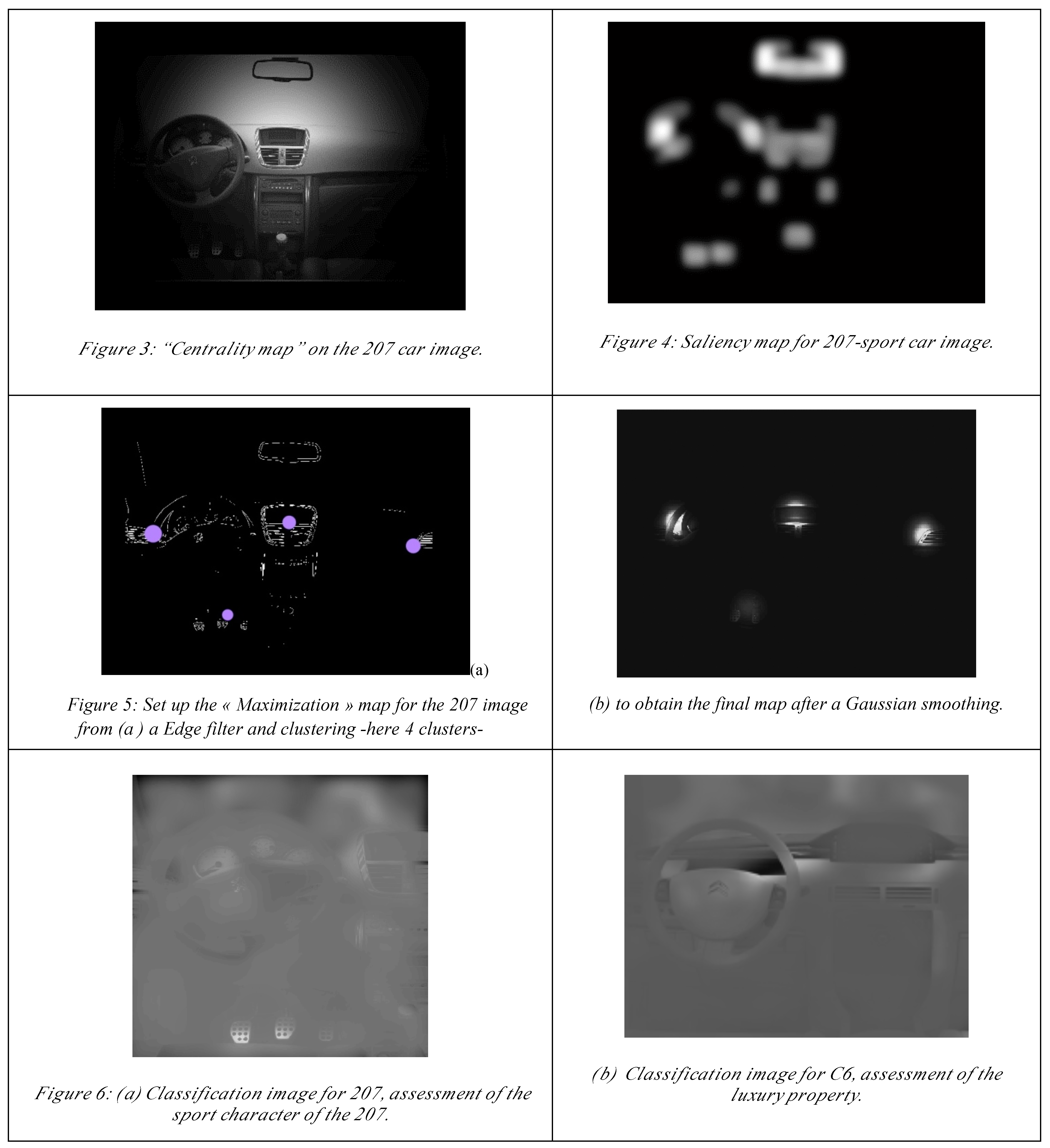

