Fractal Portfolio Optimization in the Evolving Returns Integrated System—ERIS ^†

Abstract

This paper proposes a new model with the goal of improving several aspects of the modern portfolio theory: (i) investor behavior, (ii) depiction of behavior in the fractal stochastic differential equations about price efficiency in chaotic dynamics (Tsallis statistics) and the fractal market hypothesis, (iii) the introduction of the novel Evolving Returns Integrated System (ERIS) in portfolio selection in the fractal behavioral convolution, and (iv) the selection of an accurate classifier (ERIS) among three neuro-genetic hybrids of 66 models: 22 modular, 22 Jordan–Elman and 22 generalized feedforward networks. Our model demonstrates superior classification performance across the Greek (1996–1998) and NYSE (2008–2010) equity market datasets examined in this study.

1. Introduction

A more analytical tool than currently exists is required in modern portfolio theory to resolve its inefficiencies. Portfolio selection in its final phase needs to consider more advanced aspects of risk contained in higher moments and describe their fractal behavior, which requires a more robust portfolio selection process. By proposing a new conceptual framework, this paper aims at capturing such effects and producing more accurate binary classification (into “healthy” vs. “distressed”) of a large cross-section of Greek stocks.

Following previous work (Loukeris & Eleftheriadis, 2017), leptomorphic risk meters, such as volatility, hyperkurtosis, ultrakurtosis, hyperultrakurtosis, etc., are proposed in this paper. At first, the portfolios are evaluated to form the feasible set and the efficient frontier of maximum return under minimal risk on a utility function (Loukeris & Eleftheriadis, 2015; Loukeris et al., 2024, 2025). This paper evaluates the first step, which offers the solution to the second step. The returns reflect leptomorphic aspects of behavior as an expression of gain and pain that fuses the asset fundamentals and the chaotic entropy of the public market. The novel Evolving Returns Integrated System (ERIS) is introduced to select portfolios considering the equilibrium between fractal behavioral convolution and the fundamentals of securities (Loukeris, 2023). The ERIS best classifier is selected, scrutinizing 22 modular networks (MDNs), 22 Jordan–Elman networks (JELs) and 22 generalized feedforward (GFF) hybrid neuro-genetic models in different topologies. We develop the ERIS framework and evaluate its performance across two distinct historical market regimes: the pre-euro period (1996–1998) and the systemic subprime and Eurozone debt crisis (2008–2010). The following are the specific contributions of this research:

(I)

It examines the preferences and the behavior of investors according to higher moments and their implications for profits and risk exposure.

(II)

It emphasizes isoelastic utility in practical applications.

(III)

It develops a framework similar to Markowitz’s portfolio theory but with hidden information of fundamentals to exclude the bias and detect healthy assets in the fractal market hypothesis and chaos dynamics in finance.

(IV)

It examines the efficiency of MDNs, JELs, and GFF hybrid networks as optimal classifiers in trading applications.

(V)

It proposes a new ERIS integrated system for portfolio selection.

For robustness purposes, we formulate three testable hypotheses:

Hypothesis 1. 

The JEL GA hybrid maintains its 97% classification accuracy during the 2008–2010 volatility explosion.

Hypothesis 2. 

Fractal-based models provide a better fit to equity return distributions, especially in the presence of heavy tails and skewness.

Hypothesis 3. 

The optimal model fits crisis data worse, even after accounting for complexity.

The three hypotheses developed above are grounded in the prior literature emphasizing the nonlinear and asymmetric nature of financial markets. Research on adaptive intelligent systems and chaotic market dynamics suggests that hybrid learning models may retain predictive robustness during periods of increased volatility (Atsalakis & Valavanis, 2009; Peters, 1994), thereby motivating Hypothesis 1. In addition, empirical evidence has shown that equity returns frequently exhibit excess kurtosis, skewness, and non-Gaussian behavior (Cont, 2001; Fama, 1965; Mandelbrot & Hudson, 1997), while investor preferences may also depend on higher-order moments (Harvey & Siddique, 2000), which motivates Hypothesis 2. Finally, prior studies on crisis periods and volatility clustering suggest that extreme market conditions may cause model stability and predictive ability to deteriorate despite increasing model complexity (Sornette, 2003; Taleb, 2007), thereby supporting Hypothesis 3.

A significant number of observed anomalies that financial models fail to account for in terms of the data-generating process of asset returns (Harvey et al., 2015) warrants a deeper analysis of human behavior not only with respect to asset pricing with fundamentals but also with respect to the investors’ philosophical perception of pain/gain. In general terms, philosophy and behavioral traits are present everywhere, especially when explaining patterns in the activity of investors. The portfolio selection process puts into question the free-will aspect of individual investors. Loukeris et al. (2024, 2025) answered the fundamental problem of logic in portfolio selection, concluding that logic follows a linear dynamic fitness, readjusting and overriding the new slots of superior profits in less loss coming from short memory. Superior welfare chances are also possible, but with more complexity than obtained by linear processing.

Recent advances in artificial intelligence and portfolio optimization have strongly emphasized the importance of adaptive and data-driven financial modeling approaches. For instance, the literature explores the use of deep learning architectures for portfolio optimization and financial forecasting in volatile market conditions (Lee et al., 2024; Weber et al., 2024). Also, recent research work highlights the emerging role of artificial intelligence in financial decision-making and portfolio management (Sutiene et al., 2024). Some other studies have examined the usefulness of machine learning approaches in portfolio optimization under leptokurtic distributions and market uncertainty (Habbab & Kampouridis, 2024). Lastly, explainable and hybrid intelligent models in finance have attracted a lot of attention, particularly concerning their transparency and decision-making capabilities in complex financial situations (Chen et al., 2023).

This paper is organized as follows: Section 2 discusses the behavior of investors, Section 3 discusses the model, Section 4 provides a description of MDNs and their hybrids, while Section 5 includes the partially recurrent networks—JELs. Section 6 presents more of our methodology, specifically GFFs and their hybrids. This is followed by Section 7, which is about our proposed model configuration (ERIS). Section 8 presents the dataset. Then, Section 9 shows the results of our empirical exercises, and Section 10 offers the concluding remarks.

2. Behavior of Investors in Fractal Markets

Harvey et al. (2015) report at least 316 anomalies in asset-pricing models that increase the inaccuracy of expected return predictions. This irrational behavior of investors operating under emotional biases requires a nonlinear modeling of higher complexity to describe it. The most turbulent times of the global financial crisis presented short investment horizons as in the fractal market hypothesis. Kristoufek (2013) notes that the market fails the efficient market hypothesis (EMH) given that distributions of returns are not normal, identically distributed, and independent (i.e., non-i.i.d.). As investors are more sensitive to their potential losses (Kozaki & Sato, 2008), a new model is proposed. The new paradigm of Tsallis statistics analyzes fractals in the chaotic environment of stock markets, and the fractal market hypothesis is incorporated in the new ERIS model. Investors allocate their utility, expecting a reasonable return in fear of loss, and thus make biased decisions. Investors are usually risk-averse or risk-neutral. Higher moments of returns reflect the investors’ hidden patterns on the implied utility function of the HARA (Hyperbolic Absolute Risk Aversion) form. We use higher moments than the fifth of hyperskewness (Loukeris & Eleftheriadis, 2015, 2017; Loukeris et al., 2024, 2025):

$$U_t\left(r_{p,t}\right)={\sum }_{{\lambda }_{\nu }=1}^{\omega }(-1{)}^{{\lambda }_{\nu }+1}{\displaystyle \frac{a_{{\lambda }_{\nu }}}{n}}{{\sum }_{i=1}^n\left(r_i-\sum {\displaystyle \frac{r_i}{n}}\right)}^n$$

(1)

where λ_ν is the accuracy of investors’ preferences to risk depending on behavior; a_λν is the constant of the investors’ profile, in which a_λν = 1 rational risk-averse individuals and a_λν ≠ 1 non-rational; r_i is the return of asset i at time t; and $r_{p, t}$ is the return of the investment portfolio. The isoelastic utility, a unique HARA function of Constant Relative Risk Aversion, is for risk-averse investors:

$$U=\{\begin{array}{c}{\displaystyle \frac{W^{1-\lambda }-1}{1-\lambda }}, \lambda \in (\mathrm{0,1})\cup (1,+\infty ]\\ \mathit{log}(r), \lambda =1\end{array}$$

(2)

where W is wealth and λ is a measure of risk aversion. Loukeris et al. (2024, 2025) indicated that the Markowitz model can have a broader alternative, relaxing its essential assumption on the normally distributed returns. The initial convex problem of quadratic utility maximization (Markowitz, 1952) is non-effective in the markets:

$$\mathit{min} f\left(r\right)=Var\left(r_p\right)$$

(3)

Maringer and Parpas (2009) incorporated higher-order moments:

$$\mathit{min}f\left(r\right)=\lambda Var\left(r_p\right)-(1-\lambda )E\left(r_p\right)$$

(4)

$$r_p={\sum }_i{w}_i{r}_i$$

(5)

$$w_i\ge 0$$

(6)

$${\sum }_i{w}_i=1$$

(7)

where r_p is the portfolio return, w_i is the weight of asset i, r_i is the return of the ith asset, μ is the mean and σ² is the variance. Regarding the chaotic dynamics, Tsallis (1988) relative entropy describes complex systems with nonlinearity, long-range interactions and long-term memory effects. Stock markets research on the Tsallis generalization of the Kullback–Leibler relative entropy was undertaken by Biró and Rosenfeld (2012), Kaizoji (2006), Kozaki and Sato (2008), Queirós et al. (2007), Rak et al. (2007), Tsallis et al. (2003), and Zhao et al. (2021).

Times of increased volatility (Sornette, 2003) occur relatively frequently in financial markets, probabilistically producing mispriced securities (Peters, 1994; Subrahmanyam, 2008). The emotional bias is better reflected in nonlinear dynamic models of the fractal market hypothesis (Kristoufek, 2013). Events such as the U.S.–China trade war, the Ukraine–Russia conflict, the Hamas–Hezbollah–Israel war, and the Israel–Iran–U.S. stand-off produce excessive volatility that may be exploited for short-term investments. Market prices react as multidimensional space-time fractals during such shocks, and this may result in higher price jumps and increased volatility that generates bubbles and bursts. As investors focus on their potential losses (Subrahmanyam, 2008) in chaotic market dynamics, our approach brings more efficient investment strategies, where higher moments reflect the fractal behavior of investors in the HARA utility (Loukeris & Eleftheriadis, 2017; Loukeris et al., 2024, 2025). Fractals are probabilistically self-similar distributions over their parts and the whole across different scales, appearing as natural phenomena of the markets and of nonlinear and complex behaviors, thus adding accuracy in the valuation of the return and risk in portfolios. To incorporate the fractal characteristics of return and risk, two fractal indicators are created: fractal expectation and fractal variance. These indicators will be used as optimization inputs.

The methods are as follows (Freund et al., 1999; Li & Wu, 2025): in the price trajectory with endpoints x₀ and x_T, let e = d (x, y) be the distance between points x and y, and as x₁ and x₂, the conditions d (x₀, x₁) = ε and d (x₁, x₂) = ε hold. If d (a_n, x_T) ≤ ε holds, the length of the trajectory is L(ε) = εn(ε). If ε is smaller, the curve length will be more accurate. The conventional approach shows that when $\underset{\epsilon \to 0}{\lim }L\left(\epsilon \right)=L\to 0$, where L is the length of the trajectory, as $\underset{\epsilon \to 0}{\mathit{lim}}L\left(\epsilon \right)\to \mathrm{\infty }$, L is invalid. If a > 2, E_c(X) is finite, and ⁆ E(X); otherwise, if a < 2, E_c(X)$\to \mathrm{\infty }$, then the expected value E(X)$\to \mathrm{\infty }$.

$$E_c\left(X\right)={\int }_{-c}^{c}x\rho \left(x\right)dx={\int }_{-c}^c{\rho }_0{x}^{1-\alpha }dx= {\displaystyle \frac{{\rho }_0}{2-a}}(c^{2-a}-x_0^{2-a})$$

(8)

When E(X) is finite and valid, the fractal E_f(X) = 〈$E_X, e_X$〉 return is given by:

$$\left\{\begin{array}{c}{E}_f\left(X_i\right)<E_f\left(X_j\right)\iff (e_{X_i}<e_{X_j})\bigvee [\left(e_x=e_x\right)\bigwedge \left(E_{X_i}<E_{X_j}\right)\\ E_f\left(X_i\right)E_f\left(X_j\right)=\langle E_{X_i}<E_{X_j}, e_{X_i}+e_{X_j}\rangle \\ E_f\left({\displaystyle \sum _{\iota =1}^n}{a}_{\iota }{X}_i\right)={\displaystyle \sum _{\iota =1}^n}{a}_{\iota }{E_f(X}_i)=\langle {{\displaystyle \sum _{\iota =1}^m}{a}_{i_k}{E}_{X_{i_k}},e}_{X_{\eta }}\rangle , e_{i_1}=\cdots =e_{i_m}=\max \{e_i{\}}_{i=1}^n\\ E_f\left(X_i\right)[E_f\left(X_j\right){]}^{-1}=\langle E_{X_i}{{\rm E}}_{X_j}^{-1}, e_{X_i}-e_{X_j}\rangle \\ \left[E_f\left(X_i\right){]}^q=\langle {{\rm E}}_{X_i}^{q}q{e}_{X_i}\rangle , ⩝{i\ne j⋲\{1,\dots ,n}_{i_k}\right\}\end{array}\right\}$$

(9)

The fractal variance, according to Freund et al. (1999) and Li and Wu (2025), is Var(X) = $\underset{c\to \infty }{\lim }{E}_c^2$(X) − [$\underset{c\to \infty }{\lim }{E}_c$(X)${]}^2$ if a ≠ 3:

$$\mathrm{V}\mathrm{a}\mathrm{r}(\mathrm{X})\mathrm{ }=\underset{c\to \infty }{\lim }\left[{\displaystyle \frac{{\rho }_0}{3-\alpha }}\left(c^{3-a}-x_0^{3-a}\right)- {\displaystyle \frac{{\rho }_0^2}{(2-\alpha {)}^2}}\left(c^{4-2a}+x_0^{4-2a}-2c^{2-a}{x}_0^{2-a}\right)\right]$$

(10)

and it incorporates the risk diversification of the portfolio:

$$\left\{\begin{array}{c}{Var}_f\left(X_i\right)<{Var}_f\left(X_j\right)\iff (v_{X_i}<v_{X_j})\bigvee [\left(v_{X_i}<v_{X_j}\right)\bigwedge \left(V_{X_i}<V_{X_j}\right)\\ {Var}_f\left(X_i\right)Var(X_j)=\langle V_{X_i}<V_{X_j}, v_{X_i}+v_{X_j}\rangle \\ {Var}_f\left({\displaystyle \sum _{\iota =1}^n}{a}_{\iota }{X}_i\right)={\displaystyle \sum _{\iota =1}^n}{a}_i^2{{Var}_f(X}_i)=\langle {\displaystyle \sum _{\iota =1}^m}{a_{i_k}^{2}V}_{X_{i_k}},v_{X_{\eta }}\rangle , v_{i_1}=\cdots =v_{i_m}=\max \{v_i{\}}_{i=1}^n\\ {Var}_f\left(X_i\right)[{Var}_f\left(X_j\right){]}^{-1}=\langle V_{X_i}{V}_{X_j}^{-1}, v_{X_i}-v_{X_j}\rangle \\ \left[{Var}_f\left(X_i\right){]}^q=\langle V_{X_i}^{q}q{v}_{X_i}\rangle , ⩝{i\ne j⋲\{1,\dots ,n}_{i_k}\right\}, ⩝q⋲R^{+}\end{array}\right\}$$

(11)

Conceptually, the fractal expectation and fractal variance measures (Equations (8)–(10)) serve as mathematical descriptors of the nonlinear and multiscale behavior observed in financial markets. In contrast to the standard mean-variance framework, these moments are designed to reflect fat tails and long-memory characteristics captured through the fractal market hypothesis and Tsallis statistics. Within the ERIS setting, these fractal features are used as inputs to the hybrid neural architecture, where the MDN component models probabilistic return distributions, the JEL component describes nonlinear relationships between assets, and the GFF component represents complex, dynamic interactions. Hence, the fractal measures provide a statistical characterization of real-world market structures, while the neural components learn their predictive and optimization patterns relevant for portfolio selection.

The portfolio P is composed of n assets $\{Y_i{\}}_{i=1}^n$ with weights $\{{\omega }_i{\}}_{i=1}^n$ and the return $r_{exc,i_t }$ on the assets is $\{r_{exc,i_t }{\}}_{i=1}^n$:

$$\{\begin{array}{c}\min Var\left(r_p\right)=\min \{{\displaystyle {\sum }_{\iota =1}^n}{\omega }_i^2{Var(r_{exc,i}}_t)+{\displaystyle {\sum }_{\iota =1}^n}{\omega }_i{{\omega }_{j}Cov(r_{exc,i}}_t,r_{i_t })\}\\ \mathrm{Constraint} \mathrm{Condition} \left\{\begin{array}{c}{\displaystyle {\sum }_{\iota =1}^n}{\omega }_i=1\\ \begin{array}{c}max{\displaystyle \frac{u}{V}}\\ {\omega }_i>0\end{array}\end{array}\right\}\end{array}$$

(12)

$$\left\{\begin{array}{c}{w}_i={\displaystyle \frac{u{\displaystyle {\sum }_{\iota =1}^n}{\theta }_{ij}+[[{\displaystyle {\sum }_{\iota ,j=1}^n}{\theta }_{ij}]r_j-{\displaystyle {\sum }_{\iota ,j=1}^n}{\theta }_{ij}{r}_j]+{\displaystyle {\sum }_{j=1}^n}{\theta }_{ij}[{\displaystyle {\sum }_{\iota ,j=1}^n}{{\theta }_{\iota j}r}_i{r}_j-({\displaystyle {\sum }_{\iota ,j=1}^n}{\theta }_{\iota j}{r}_j)r_j)]}{({\displaystyle {\sum }_{\iota ,j=1}^n}{{\theta }_{\iota j}r}_i{r}_j)({\displaystyle {\sum }_{\iota ,j=1}^n}{\theta }_{\iota j})-({\displaystyle {\sum }_{\iota ,j=1}^n}{\theta }_{\iota j}{r}_j{)}^2}}\\ \left[\begin{array}{c}{\theta }_{11} {\theta }_{12}\dots {\theta }_{1n}\\ \begin{array}{c}{\theta }_{21} {\theta }_{22}\dots {\theta }_{\begin{array}{c}2n\\ .\\ .\\ ;\end{array}}\\ {\theta }_{n1} {\theta }_{n2}\dots {\theta }_{nn}\end{array}\end{array}\right]={\left[\begin{array}{c}Var\left(r_{1_t}\right) Cov\left(r_{1_t},r_{2_t}\right)\dots Cov\left(r_{1_t},r_{n_t}\right)\\ \begin{array}{c}Cov\left(r_{2_t},r_{1_t}\right) Var\left(r_{2_t}\right)\dots Cov\left(r_{2_t},r_{n_t}\right)\\ Cov\left(r_{n_t},r_{1_t}\right) Cov\left(r_{n_t},r_{2_t}\right)\dots Var\left(r_{n_t}\right)\end{array}\end{array}\right]}^{-1}\end{array}\right\}$$

(13)

The assets follow a fractal distribution, overcoming traditional models where risk and return are fractals but are examined inaccurately as real moments. The portfolios in fractal form balance better return and risk in a more efficient assessment. Fractals provide a closer-to-reality tool to analyze the peak-fat-tails extreme-event characteristics in financial markets. The uncertainty and the fat tails of a higher possibility of extreme losses make investor barriers necessary to protect them from potential extended losses. Market risks require a thorough examination of their asymmetry by peak-fat-tails and robust strategies (de Prado, 2018; Heaton et al., 2017; Mandelbrot & Hudson, 1997; Peters, 1994; Rumelhart et al., 1986).

When compared with existing fractal- and machine-learning-based portfolio optimization approaches, the proposed ERIS framework provides a more general treatment of market complexity and its nonlinear dynamics. Traditional fractal models mainly focus on long-memory behavior and multiscale properties of returns, whereas the goal of machine learning approaches is often superior predictive performance, but without incorporating non-extensive distributional characteristics of returns observed in financial markets. To utilize these individual characteristics, ERIS combines the fractal market hypothesis that includes Tsallis statistics and hybrid neural architectures, including MDNs, JELs, and GFFs, within a unified adaptive framework. Such a combination enables the model to better capture leptokurtic properties of returns, regime shifts, and nonlinear dynamics in asset returns. As a result, the framework jointly addresses both the statistical irregularities in return distributions and the dynamic structural features of financial markets in the portfolio selection process.

3. The Model

Loukeris et al. (2024, 2025) showed that further higher moments are necessary to describe the behavior of investors:

$$\begin{array}{cc}\hfill {\mathit{min}}_{w}f\left(w\right)& =\lambda {\upsilon }_{\gamma }\left[bVa{r}_t\left(r_p\right)+dKur{t}_t\left(r_p\right)+fHypKur{t}_t\left(r_p\right)-hUltraKur{t}_t\left(r_p\right)\right]-\hfill \\ & (1-\lambda ){\upsilon }_{\gamma }\left[a{E}_t\left(r_p\right)+cSke{w}_t\left(r_p\right)+eHypSke{w}_t\left(r_p\right)+gUltraSke{w}_t\left(r_p\right)\right]\hfill \end{array}$$

(14)

$${\upsilon }_{\gamma }=1-{\epsilon }_{\tau }$$

(15)

$$r_p={\sum }_i{w}_i{r}_i^{*}$$

(16)

where υ_γ is a company’s financial health (binary: “0” bankrupt, “1” healthy); ε_τ is the heuristic output as the evaluation result (binary: “0” healthy, “1” distressed); r_i^* is the return of stock i, which is from the efficient frontier and is superior to the others; and w_i’s are their weights. Hence:

$${U_t(r}_p)={\sum }_i{U}_t\left({R_t(i}_i^{*}\right))$$

(17)

The non-convex problem demands robust heuristics, where we contribute with a more efficient hybrid classifier that also considers hidden accounting information among the ordinal data and detects possible creative accounting or corporate manipulation. Hence, malicious processes that are fraudulent and misleading to the investors are restricted.

4. MDNs and Their Hybrids

MDNs are a special class of multilayered perceptrons (MLPs) that process their inputs using several parallel MLPs and then combine the results (Figure 1). This tends to create some structure within the topology, which fosters specialization of a functional form in each module. In each module, the number of hidden layers and the network topology can be defined. In contrast to MLPs, MDNs do not have full interconnectivity between their layers. Therefore, a smaller number of weights is required for the same size of network (same number of neurons). This tends to speed up training times and reduce the size of the training dataset. There are various criteria to segment an MLP into modules, and there is a degree of subjectivity involved in how to best design the modular topology based on data. The modules of an MDN could be overlapping and they do not have to be trained on unique portions of data.

Our MDN setting is as follows: 16 input neurons, 1 output; training data: 706 observations. As for hidden layers, we include 4 neurons in the upper/lower parts with the hyperbolic tangent transfer function (TanhAxon). The learning rule momentum was set at step size 0.1 and a momentum of 0.70. Backpropagation is used as ordinal learning, and the connection weights are changed according to their previous value and correction term. The supervised learning used the maximum of 1000 epochs and the convergence criterion was the mean-squared error (MSE). The minimum threshold was set at 0.01 in batch learning.

The maximum number of epochs defines the number of iterations (on the training set) to be done if the convergence criterion is not met. The training algorithm terminates when the MSE drops below the specified threshold. Alternatively, the MSE can terminate training depending on the stop criteria for cross-validation data instead of that for the training set. Thus, when the MSE of the cross-validation set starts to increase, it indicates that the network is overtraining (i.e., incapable of generalizing the input–output relationship).

5. Partially Recurrent Networks: JELs

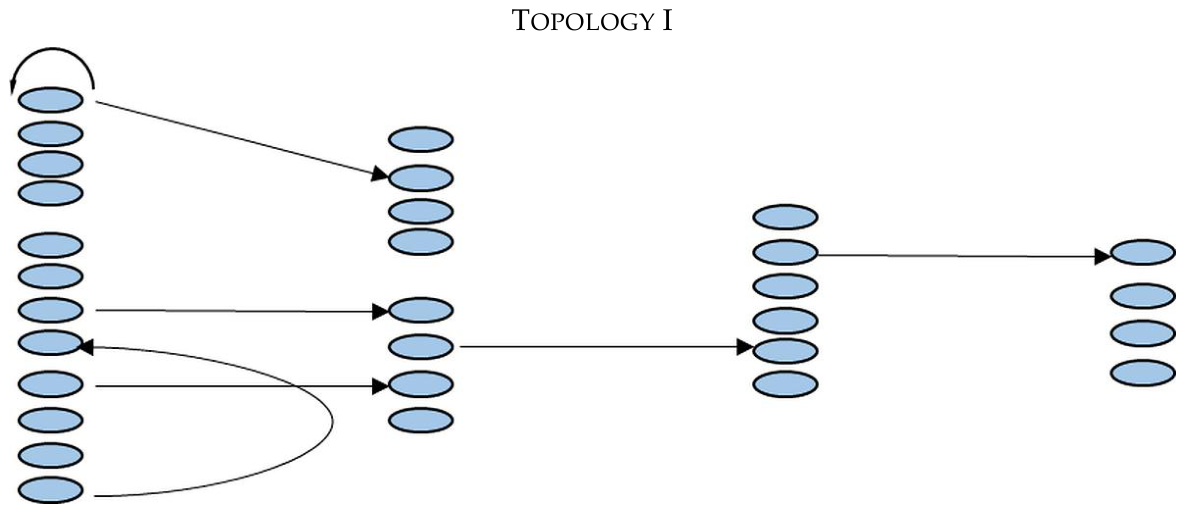
Partially recurrent networks are MLPs where a few recurrent connections are introduced (Figure 2). The recurrent networks include two types of neurons: the neurons that behave as inputs, receiving external signals, and the context neurons or neurons of state, which remember past actions and take output values from one of the layers delayed by one step. Internal states, which function as short-term memory of the partially recurrent neural nets, can predict time series, as they can represent information about the preceding inputs (Stagge & Sendhoff, 1997). The types of partially recurrent networks are: (i) the Jordan network, (ii) the Elman network, and (iii) the multi-step recurrent network. The Jordan-and-Elman-type networks, or JELs, extend MLPs by implementing neurons that remember past activity, also called the context units (Loukeris et al., 2024, 2025). These units offer the ability to extract temporal information from the data and input it to JELs. We tested four JEL topologies based on the number of layers that feed the context units. The context neuron memorizes the past of its inputs in the recency gradient, which uses the forgetting factor in an exponential decay mode. Here, the idea is that the memory of recent data is more informative than the memory of those in a more distant past. The neurons of the context unit manage the forgetting factor as a constant that takes values between 0 and 1. In the case of 0, only the present-time data are considered, indicating that there is no recurrent connection, while for a value of 1, all of the past is factored in. The closer the value is to 1, the longer the memory depth and the slower the forgetting factor. The number of neurons in the context layer is defined by the number of neurons in the layer that feeds the context layer. As is the case with other neural network models, the number of hidden layers must be defined. The configuration of all JELs in the current research is selected to feed the context units with input variables (or predictors).

We selected a forgetting factor of 0.8 s, and the number of neurons in the hidden layer was set to 4 with the hyperbolic tangent transfer function (TanhAxon). The learning rule was the momentum function with a value of 0.7, and the changing step size per hidden layer was 0.1.

The significance of each of the 16 financial inputs in all JELs was calculated through the GAs for the hybrid models only. These models were trained repeatedly until they chose the inputs’ combination that produces the lowest error. The GAs were incorporated in two different hybrid models of different topologies: (1) in all layers, (2) in all layers with cross validation. Batch learning was preferred to update the weights of hybrid neuro-genetic JELs after the presentation of the entire training set. GAs also resolved the problem of optimal parameter values in all hidden layers and the output layer.

6. GFFs and Their Hybrids

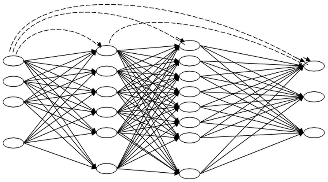
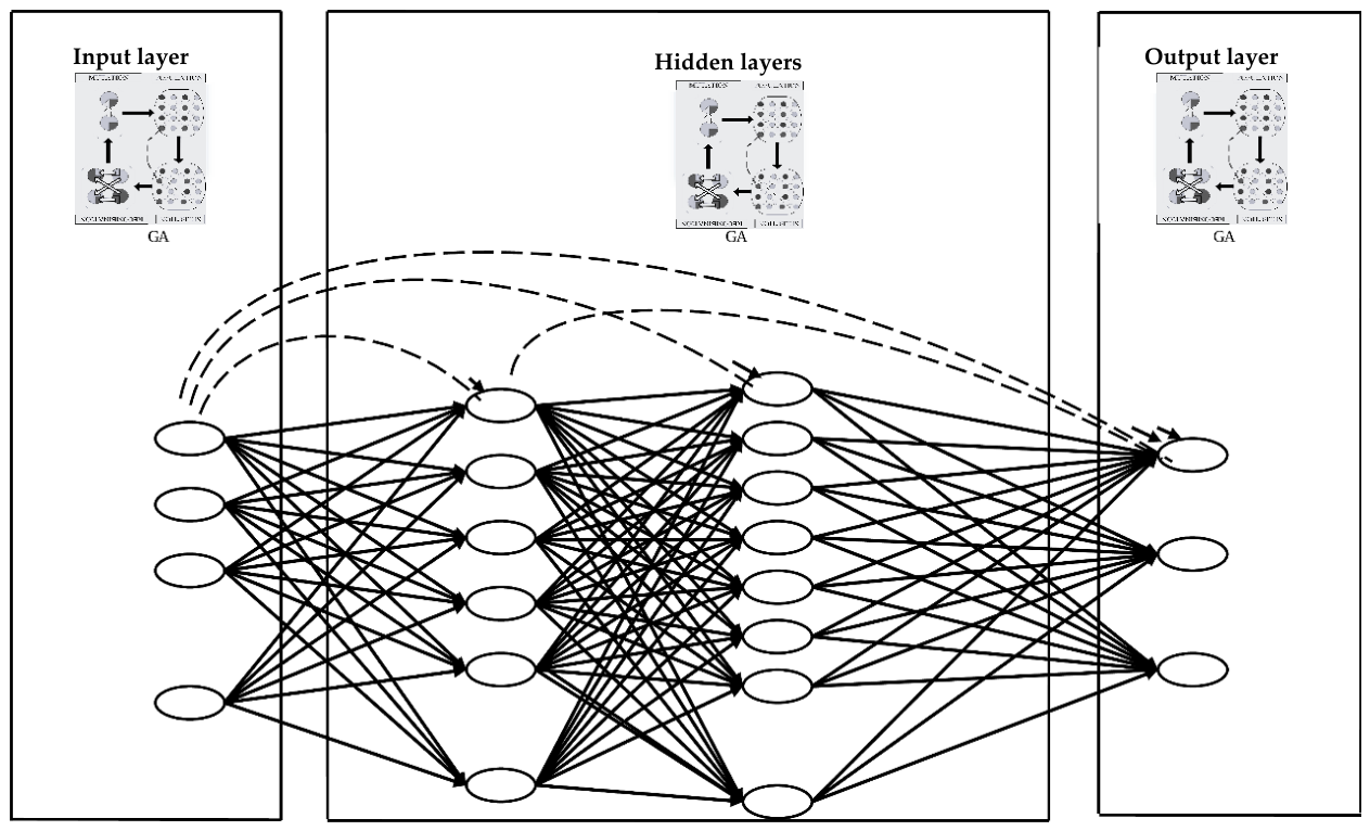
GFFs are MLPs with a generalized ability of their connections to jump over one or more layers (Figure 3). GFFs will create an MLP where each layer feeds the others, with the ability to surpass the succession of layers and form synapses with deeper layers. After the number of layers is set, the MLP requires a significantly higher training time (number of epochs) than a GFF with the same number of neurons.

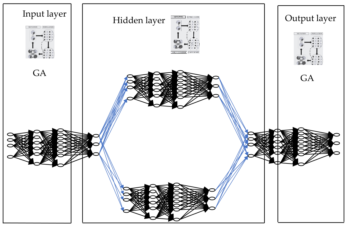
MLPs can solve similar problems to GFFs, although GFFs often provide solutions with higher efficiency. Furthermore, GFFs can be combined with GAs in a hybrid model called a hybrid GFF with GA optimization and cross validation (Figure 4). This method combines the architectural flexibility of GFFs with the optimization power of GAs for hyperparameter tuning, while the robust evaluation is provided by cross validation applied systematically throughout the GFF’s layers.

7. The ERIS

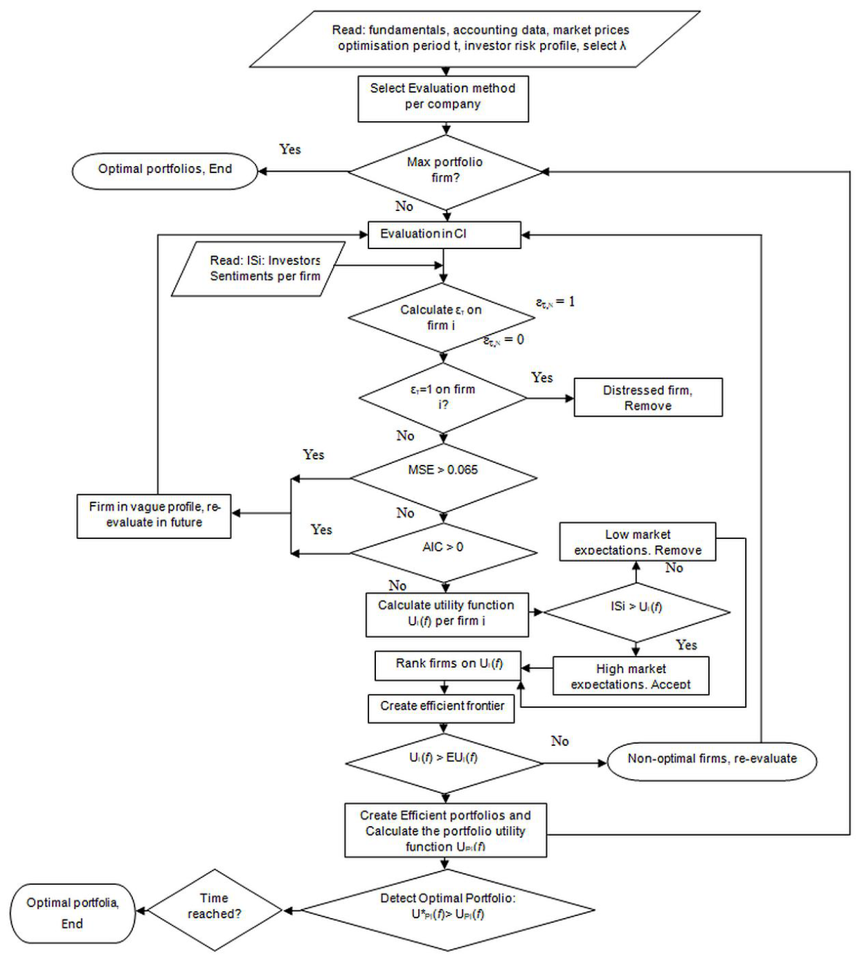
The integrated ERIS model, depicted in Figure 5, first receives the fundamentals, prices and optimization time t. It chooses the initial classifier on the stocks, taking the risk profile of each investor as well as the isoelastic utility λ. Next, ERIS tests if this is the last company of the dataset and if the optimal portfolio condition as the efficient portfolio is satisfied. This is followed by reading the investor sentiments for each stock IS_i, and from this, the algorithm moves towards the classifier that generates two subsets: subset 1 includes healthy stocks (ε_τ =0), while subset 2 includes distressed ones (ε_τ =1). If ε_τ = 1, a stock is removed, while if ε_τ = 0, this indicates that it is healthy, and it is counted as a candidate for the efficient portfolio.

The algorithm then flows to U_t (R_t(i)) representing the utility function that is produced for each stock i. Essentially, U_t (R_t(i)) is compared to IS_i while keeping prospective stocks. The stocks are ranked based on the utility score that is used to produce the efficient frontier. More specifically, stocks with the highest utility score are selected for the efficient portfolio. Then all remaining stocks are fed back and reevaluated with potential new data by using neural nets. In the end, the efficient portfolio is created, its utility function is calculated UP_j(f) and the optimal overall portfolio U*P_j(f) with maximum utility is found.

8. Data

The data were collected annually for 1411 companies from the loan department of a Greek commercial bank (Emporiki Commercial Bank, acquired by Alpha Bank in 2012), with the following financial indicators spanning the 1996–1998 period (three-year averages were used and their descriptive statistics are displayed in

Table 1. Descriptive statistics using daily data.

Statistics	Sample 1 (Greece: 1996–1998)	Sample 2 (NYSE: 2008–2010)
Number of firms	1411	210
Average return	0.15%	0.02%
Average volatility	1.7%	3.1%
Average skewness	0.41	−0.40
Average kurtosis	20.41	10.12

, Courtis, 1978): (1) EBIT/Total Assets, (2) Net Income/Net Worth, (3) Sales/Total Assets, (4) Gross Profit/Total Assets, (5) Net Income/Working Capital, (6) Net Worth/Total Liabilities, (7) Total Liabilities/Total Assets, (8) Long-Term Liabilities/(Long-Term Liabilities + Net Worth), (9) Quick Assets/Current Liabilities, (10) (Quick Assets—Inventories)/Current Liabilities, (11) Floating Assets/Current Liabilities, (12) Current Liabilities/Net Worth, (13) Cash Flow/Total Assets, (14) Total Liabilities/Working Capital, (15) Working Capital/Total Assets, (16) Inventories/Quick Assets, and (17) the Bank’s index with initial classification, estimated by the bank’s experts. The testing set was 50% of the overall data, and the training set was the remaining 50%. All 17 numerical inputs produced an integer outcome as an evaluation ε_τ [“0”: healthy, “1”: distressed], so there was no need to normalize them. In addition, it is worth stressing that the hybrid models utilized in this paper can process noisy and non-stationary inputs without the necessity to winsorize or normalize them. The training set had 706 firms, or 50.03% (597 healthy and 109 distressed), the testing set had 705, or 49.96% (596 healthy and 109 distressed), and the cross-validation set had 160 firms, or 11.33% (119 healthy and 41 distressed). During the training phase, 1000 repetitions (epochs) were used with early stopping cross validation.

In addition to the Greek dataset, we introduced a sample comprising 210 NYSE-listed stocks over the 2008–2010 period. This was done to evaluate the ERIS framework across distinct market environments and jurisdictions representing structurally different regimes with differing accounting and regulatory frameworks, including the pre-IFRS reporting environment in the Greek market. In effect, we evaluated the ERIS framework under varying institutional and regulatory conditions rather than focusing on direct cross-period comparability or contemporary forecasting performance. Firm characteristics similar to the 17 financial ratios used for the Greek companies were again considered. The training/testing data partition also remained unchanged, with 50% allocated to each subset.

We compare the two samples in Table 1. The average figures suggest that the Greek market produced higher returns but a lower standard deviation compared to the NYSE sample. However, the observed level of volatility in the Greek market (1.7% daily standard deviation) remains economically meaningful, reflecting the market’s emerging structure, lower liquidity, and higher informational frictions during the period. In contrast, the 2008–2010 NYSE sample reflects elevated systemic stress during the global financial crisis, with a substantially higher dispersion of returns. As far as skewness is concerned, Greece showed positive skew where upside movements were dominant, while the NYSE market was also asymmetric, with downside risk being present. Both markets were characterized by high kurtosis indicating non-normal return distributions. While NYSE experienced a globally more significant crisis, its institutional structure somewhat compressed tail risk compared to a more speculative emerging market in Greece.

Although the selected data periods provide coverage of two distinct market regimes, the analysis remains potentially sensitive to limitations related to sample size and representativeness. In particular, the NYSE dataset relies on a smaller cross-section taken around the global financial crisis, which may influence the stability and generalizability of the results. We wish to stress that the above-outlined cross-validation and calibration procedures were designed to reduce overfitting risk. Nevertheless, we acknowledge that additional validation using larger and more diverse contemporary datasets across multiple market regimes would further strengthen the robustness assessment of the proposed ERIS framework, but we leave such explorations to future research.

Finally, we acknowledge that financial markets and regulatory frameworks have evolved substantially since the sample periods used in this paper. Specifically, post-crisis regulatory reforms and the rise of algorithmic and high-frequency trading driven by artificial intelligence have significantly impacted financial market structure. While these changes may influence specific investment performance, the core nonlinear and fractal characteristics of asset returns have remained well-defined across a wide range of markets and time periods. Notwithstanding these considerations, further testing of the proposed ERIS framework in modern markets and regulatory frameworks constitutes an important direction for future research.

We find it worthwhile to note that sample 1 can be viewed as “Phase 1: Framework development and calibration” and sample 2 as “Phase 2: Systemic financial shock”.

9. Discussion of Results

For Phase 1, the hybrid JEL model with one GA layer demonstrated superior classification ability with respect to the healthy and distressed assets at 99.91% and 95.41%, respectively (

Table A1. Panel (A). Phase 1: Optimal models of MDN, SOFM, and GFF. Panel (B). Phase 2: Optimal models MDN, SOFM, and GFF in new NYSE data. Panel (C). Comparative analysis across regimes (phases).

(A)
Models		Active Confusion Matrix				Performance						Time
	Layers	0 → 0	0 → 1	1 → 0	1 → 1	MSE	NMSE	r	%Error	AIC	MDL
JEL GA All	1	99.91	0.08	4.58	95.41	0.24	0.56	0.975	14.03	−556.54	−233.44	1 h 38′ 53″
GFF GA All	3	97.14	2.84	17.88	82.10	0.14	0.33	0.986	8.34	−393.18	284.34	2 h 44′ 43″
MDN GA All	2	97.56	2.43	18.8	81.19	0.12	0.29	0.967	7.26	−533.73	71.40	18 h 29′ 29″
(B)
Models		Active Confusion Matrix				Performance						Time
	Layers	0→0	0→1	1→0	1→1	MSE	NMSE	r	%Error	AIC	MDL
JEL GA All	1	100	0	7.62	92.30	0.02	0.15	0.920	1263.70	−133.49	−82.41	4 h 05′ 24″
GFF GA All	3	98.97	1.02	30.76	69.23	0.06	0.40	0.822	1667.89	1916.12	2310.98	5 h 32′ 50″
MDN GA All	2	100	0	46.15	53.84	0.05	0.34	0.811	1324.48	1974.24	2382.57	3 h 22′ 06″
(C)
	Phase 1 (1996–1998)						Phase 2 (2008–2010)
Optimal model	JEL GA All						JEL GA All
Complexity	1						1
AIC	−556.54						−133.49
MSE	0.24						0.02
r	0.975						0.92
0 → 0 (1 → 1)	99.91% (95.41%)						100% (92.30%)

A). The fitness of the model to the data was 0.975, and the lowest MSE was at 0.24, where the normalized MSE (NMSE) and accuracy (%error) were 0.56 and 14.03%, respectively. The AIC value was low at −556.56 with a training time of 1 h:38 min:53 s.

The second rank was given to the hybrid GFF with GA optimization that includes three GA layers. This model resulted in a highly efficient classification, the highest fitness to the data (r = 0.986), lower MSE, and a processing time of 2 h:44 min:43 s.

We interpret the results as evidence that the hybrid JEL networks were better able to generalize across the examined financial environments and filter potentially noisy cross-sectional fundamental information averaged over the three-year period. In contrast, the deeper structure of the hybrid GFF networks may have captured more complex relationships among the inputs, but at the cost of diminished generalization capability under heterogeneous market conditions. It is noteworthy that the temporal architecture of JELs may also have contributed to more stable classification behavior in the presence of nonlinear financial dynamics.

The third rank was given to the hybrid MDN net with two layers, with a weaker classification ability, fitness, and error performance. Also, the training time was longer at 18 h:29 min:29 s. Overall, hybrid GFFs had superior performance compared with the hybrid MDN models (

Table A2. Phase 1: Modular hybrid networks overall.

Models		Active Confusion Matrix				Performance						Time
	Layers	0 → 0	0 → 1	1 → 0	1 → 1	MSE	NMSE	r	%Error	AIC	MDL
MDN GA All	0	100	0	100	0	0.56	1.33	0	12.84	−374.26	−355.71	46′ 13″
	1	98.99	1.00	59.62	40.36	0.24	0.56	0.646	14.03	−556.54	−233.44	9 h 20′ 55″
	2	97.56	2.43	18.8	81.19	0.12	0.29	0.967	7.26	−533.73	71.40	18 h 29′ 29″
	3	98.57	1.42	27.52	72.47	0.14	0.33	0.880	6.61	1505.40	3366.33	11 h 23′ 47″
	4	99.58	0.41	71.55	28.43	0.32	0.77	0.522	14.96	2629.15	4828.56	16 h 27′ 45″
	5	100	0	98.16	1.83	0.42	0.98	0.124	19.31	3841.28	6693.77	24 h 33′ 30″
	6	100	0	100	0	0.46	1.09	0	14.30	5183.69	8850.47	28 h 32′ 49″
	7	100	0	99.54	0.45	0.49	1.17	0.088	16.16	5650.55	9589.66	33 h 52′ 32″
	8	100	0	100	0	0.48	1.13	0	16.35	5218.68	8895.64	38 h 6′ 47″
	9	100	0	100	0	0.42	1.00	0	19.59	9451.22	15,885.74	55 h 27′ 51″
	10	100	0	100	0	0.42	0.99	0	19.54	6962.83	11,807.26	50 h 56′ 12″
MDN GA ALL CV	0	99.16	0.83	66.51	33.48	0.37	0.86	0.584	11.49	−813.49	−798.78	21′ 36″
		99.07	0.92	67.42	32.56	0.37	0.86	0.581	11.36	−827.78	−813.07
	1	98.49	1.50	30.72	69.26	0.15	0.35	0.862	9.98	−823.24	−489.26	3 h 30′ 54″
		97.90	2.09	30.73	69.26	0.15	0.36	0.883	7.93	−804.47	−470.58
	2	99.08	0.92	59.17	40.82	0.34	0.80	0.649	10.35	−146.62	367.12	7 h 04′ 56″
		98.49	1.50	57.79	42.19	0.35	0.82	0.683	10.91	−100.01	413.66
	3	97.98	2.01	23.84	76.14	0.15	0.35	0.922	7.55	537.19	1749.41	15 h 16″ 39″
		98.07	1.92	25.04	74.94	0.14	0.33	0.911	9.09	511.92	1724.54
	4	100	0	99.54	0.45	0.40	0.94	0.062	19.62	2096.28	3853.08	15 h 56′ 35″
		99.78	0.25	98.62	1.37	0.40	0.95	0.152	19.71	2101.90	3858.48
	5	100	0	100	0	0.42	0.99	0	19.48	2262.26	4104.55	17 h 38′ 23″
		100	0	100	0	0.42	0.99	0	19.49	2263.12	4104.69
	6	100	0	97.70	2.29	0.35	0.82	0.139	19.58	4071.90	7153.52	20 h 49′ 32″
		99.74	0.25	95.41	4.58	0.34	0.81	0.225	18.40	4057.16	7138.67
	7	100	0	100	0	0.41	0.96	0	19.27	5527.14	9470.75	31 h 43′ 43″
		100	0	100	0	0.40	0.95	0	19.53	5517.16	9460.10
	8	99.91	0.08	90.82	9.17	0.37	0.88	0.287	21.14	3317.51	5886.71	15 h 06′ 31″
		100	0	100	0	0.45	1.06	0	15.13	3451.22	6020.31
	9	100	0	100	0	0.47	1.12	0	15.97	4832.44	8268.67	11 h 56′ 27″
		100	0	100	0	0.47	1.12	0	16.19	4830.53	8266.24
	10	100	0	99.08	0.91	0.42	0.99	0.088	19.47	8288.00	13,981.80	83 h 13′ 35″
		100	0	99.54	0.45	0.42	0.99	0.062	19.42	8289.22	13,982.53

,

Table A3. Phase 1: Jordan–Elman hybrid networks overall.

Models		Active Confusion Matrix				Performance						Time
	Layers	0 → 0	0 → 1	1 → 0	1 → 1	MSE	NMSE	r	%Error	AIC	MDL
JEL GA All	0	100	0	100	0	0.560	1.33	0	12.84	−374.26	−355.71	1 h 27′ 28″
	1	99.91	0.08	4.58	95.41	0.240	0.56	0.975	14.03	−556.54	−233.44	1 h 38′ 53″
	2	99.83	0.16	33.48	66.50	0.120	0.29	0.797	7.26	−533.73	71.40	2 h 26′ 13″
	3	100	0	100	0	0.140	0.33	0	6.61	1505.40	3366.33	2 h 44′ 43″
	4	100	0	100	0	0.320	0.77	0	14.96	2629.15	4828.56	2 h 31′ 22″
	5	100	0	100	0	0.420	0.98	0	19.31	3841.28	6693.77	4 h 00′ 36″
	6	100	0	99.54	0.45	0.460	1.09	0.062	14.30	5183.69	8850.47	4 h 23′ 09″
	7	100	0	100	0	0.490	1.17	0	16.16	5650.55	9589.66	5 h 18′ 38″
	8	100	0	100	0	0.480	1.13	0	16.35	5218.68	8895.64	5 h 59′ 49″
	9	100	0	100	0	0.420	1.00	0	19.59	9451.22	15,885.74	6 h 51′ 26″
	10	100	0	100	0	0.420	0.99	0	19.54	6962.83	11,807.26	7 h 36′ 09″
JEL GA ALL CV	0	100	0	100	0	0.565	1.34	0	12.85	−354.28	−324.23	1 h 05′ 02″
		100	0	100	0	0.565	1.34	0	12.85	−354.29	−324.23
	1	99.91	0.08	52.75	47.24	0.221	0.52	0.659	29.54	−1437.44	−1333.82	1 h 48′ 31″
		99.91	0.08	50.45	49.53	0.228	0.54	0.676	30.36	−1463.55	−1359.93
	2	98.82	1.17	51.37	48.62	0.023	0.06	0.713	12.32	−2439.55	−2287.32	2 h 35′ 29″
		99.83	0.16	0.91	99.08	0.023	0.06	1	28.51	−2425.75	−2273.55
	3	99.58	0.41	51.37	48.62	0.217	0.52	0.683	23.65	−1557.83	−1437.60	3 h 23′ 49″
		99.83	0.16	50.45	49.54	0.221	0.52	0.680	23.30	−1507.41	−1387.14
	4	100	0	52.75	47.24	0.422	0.99	0.656	19.59	−338.18	−86,569.10	4 h 11′ 53″
		100	0	100	0	0.422	0.99	0	19.59	−351.67	−188.54
	5	100	0	100	0	0.422	0.99	0	19.59	−275.64	4514.02	5 h 37′ 01″
		100	0	100	0	0.421	0.99	0	19.57	−278.355	5284.53
	6	100	0	98.16	1.83	0.417	0.98	0.124	19.37	−271.89	−729.14	6 h 31′ 51″
		100	0	99.54	0.45	0.420	0.99	0.062	19.44	−266.39	5857.26
	7	100	0	100	0	0.422	0.99	0	19.59	−204.67	52,493.00	7 h 42′ 32″
		100	0	100	0	0.423	0.99	0	19.61	−204.65	26,608.43
	8	100	0	100	0	0.422	0.99	0	19.59	−182.62	29,241.43	8 h 36′ 25″
		100	0	100	0	0.422	0.99	0	19.59	−182.64	30,007.15
	9	100	0	100	0	0.422	0.99	0	19.59	−142.65	154.17	9 h 49′ 48″
		100	0	100	0	0.422	0.99	0	19.59	−142.62	154.19
	10	100	0	100	0	0.422	0.999	0	19.59	−39.61	169,462.80	11 h 06′ 08″
		100	0	100	0	0.422	0.999	0	19.59	15,695.12	168,727.50

and

Table A4. Phase 1: Generalized feedforward hybrid networks overall.

Models		Active Confusion Matrix				Performance						Time
	Layers	0 → 0	0 → 1	1 → 0	1 → 1	MSE	NMSE	r	%Error	AIC	MDL
GFF GA All	0	100	0	100	0	0.56	1.33	0	12.85	2193.69	3854.24	1 h 9′ 52″
	1	97.56	2.42	18.80	81.18	0.24	0.56	0.967	8.24	−723.48	−271.82	3 h 19′ 25″
	2	98.15	1.84	23.84	76.14	0.12	0.29	0.917	8.33	−487.12	91.17	5 h 19′ 50″
	3	97.14	2.84	17.88	82.10	0.14	0.33	0.986	8.343	40,259.12	284.35	4 h 20′ 25″
	4	99.24	0.75	51.83	48.16	0.32	0.77	0.693	12.35	446.81	1493.98	10 h 57′ 50″
	5	97.56	2.42	23.85	76.14	0.42	0.98	0.936	9.75	1822.14	3844.69	18 h 24′ 19″
	6	98.99	1.00	60.09	39.91	0.46	1.09	0.642	10.87	869.02	2013.58	18 h 54′ 06″
	7	98.31	1.67	24.31	75.68	0.49	1.17	0.908	8.16	3324.09	6363.69	30 h 32′ 35″
	8	98.57	1.42	26.6	73.39	0.48	1.13	0.885	8.33	1262.65	2959.69	29 h 50′ 17″
	9	99.41	0.58	59.17	40.82	0.42	1.00	0.632	10.61	4935.72	8700.44	40 h 44′ 43″
	10	98.90	1.09	57.33	42.66	0.42	0.99	0.667	10.52	4061.09	7285.97	52 h 38′ 4″
GFF GA ALL CV	0	100	0	100	0	0.35	0.84	0	10.83	−858.23	−845.43	44′ 45″
		98.99	1.00	61.92	38.07	0.35	0.83	0	10.97	−876.9	−864.11
	1	97.98	2.00	24.30	75.68	0.15	0.34	0.659	8.65	−1219.07	−1126.30	2 h 27′ 41″
		98.4	1.59	24.76	75.22	0.13	0.33	0.676	8.69	−1242.55	−1149.79
	2	98.49	1.51	55.50	44.49	0.34	0.81	0.713	10.25	−540.53	−292.27	2 h 58′ 37″
		99.07	0.92	59.17	40.82	0.34	0.81	0.683	10.65	−528.37	−280.21
	3	97.23	2.76	26.14	73.85	0.36	0.86	0.680	11.90	28,934.43	815.64	9 h 39′ 00″
		99.32	0.67	69.26	30.73	0.35	0.84	0.656	11.75	23,234.16	803.09
	4	99.91	0.58	78.89	21.09	0.17	0.42	0	10.39	186.67	1093.18	12 h 55′ 25″
		98.48	1.51	40.36	59.63	0.18	0.43	0	11.26	216.78	1123.24
	5	97.15	2.84	20.63	79.35	0.35	0.84	0	10.23	54.02	633.59	12 h 54′ 41″
		98.90	1.09	61.00	38.98	0.34	0.81	0.124	10.81	8.31	587.91
	6	99.83	0.16	98.16	1.83	0.56	1.32	0.062	12.79	6194.21	10,418.86	37 h 53′ 44″
		100	0	100	0	0.56	1.33	0	12.85	6201.12	10,423.42
	7	96.64	3.35	19.26	80.73	0.13	0.32	0	9.12	1541.07	3429.31	25 h 46′ 34″
		98.32	1.67	29.35	70.63	0.14	0.35	0	7.07	1608.29	3495.49
	8	98.82	1.17	59.17	40.82	0.56	1.33	0	12.85	9478.70	15,799.81	34 h 09′ 15″
		100	0	100	0	0.56	1.33	0	12.92	9478.35	15,798.24
	9	99.83	0.16	99.08	0.91	0.56	1.33	0	12.89	2760.59	4783.53	8 h 32′ 59″
		100	0	100	0	0.56	1.33	0	12.87	2759.81	4782.50
	10	98.65	1.34	63.76	36.23	0.15	0.36	0	9.43	1774.06	3753.92	88 h 20′ 5″
		98.48	1.51	34.86	65.13	0.15	0.36	0	8.95	1783.68	3762.44

).

For Phase 2, a new series of experiments was performed on 210 NYSE stocks from the 2008–2010 time period. The results are shown in Table A1B, and they demonstrate the domination of the JEL hybrid model with one layer and GA in all layers (with the highest value of r = 0.92). The classification ability of the optimal model is excellent, with a 100% classification rate for healthy companies and 92.30% for distressed companies. Also, the ranking of models exhibits similar efficiency: the JEL hybrid model with one layer and GA in all layers was the most parsimonious (AIC = −133.49), yielding very low MSE error (0.022) and a medium convergence time of 4 h:5 min:24 s. The second rank was achieved by the hybrid GFF with three GA layers with an exceptional classification for the healthy companies (98.97%) and a classification of 69.23% for the distressed companies. The model fitness was high (r = 0.822), and the convergence time was 5 h:32 min:50 s. The third rank was reserved for the hybrid MDN net with two layers and GA optimization in all layers: 98.97% of the healthy companies were correctly classified, while the corresponding figure for the distressed companies was only 53.84%. The model fitness was solid at r = 0.811, but the AIC was very high (AIC = 1974.2).

Table A1C compares the optimal models for Phase 1 and Phase 2. Regarding model complexity, both phases are well explained by a robust global classifier such as the recurrent JEL model, which exhibits a more adaptive architecture, relative to the simpler, feedforward (GFF) architecture. This results in an increased classification accuracy for both healthy and distressed companies, where we conclude that the findings support Hypothesis 1. Next, we compare the AIC figures for the two phases. Clearly, the AIC in Phase 2 is lower than in Phase 1 (−556.54 < −133.49), indicating that the optimal model in Phase 2 achieves an improved balance between goodness of fit and model complexity. At the same time, the out-of-sample r for Phase 1 is higher than that in Phase 2 (0.975 > 0.92), which lends support to Hypothesis 3. In all, we can conclude that introducing fractal-based behavior into the ERIS model improves portfolio selection during crisis times (Hypothesis 2). For practitioners, these results suggest that the complexity of the ERIS model should be adjusted when transitioning from normal to crisis regimes.

The additional classification metrics for Phase 1 shown in

Table A5. Panel (A). Phase 1: Optimal models with additional metrics. Panel (B). Phase 2: Optimal models with additional metrics.

(A)
Model	Accuracy (%)	Precision (%)	Recall/Sensitivity (%)	Specificity (%)	F1-Score (%)
JEL GA All	97.67	99.92	95.42	99.92	97.62
GFF GA All	89.64	96.66	82.12	97.16	88.80
MDN GA All	89.38	97.09	81.20	97.57	88.44
(B)
Model	Accuracy (%)	Precision (%)	Recall/Sensitivity (%)	Specificity (%)	F1-Score (%)
JEL GA All	96.19	100.00	92.38	100.00	96.04
GFF GA All	84.11	98.55	69.24	98.98	81.33
MDN GA All	76.92	93.10	53.85	96.15	68.18

A indicate that the JEL GA All model achieved the strongest overall predictive performance, exhibiting the highest accuracy, recall (sensitivity), and F1-score, while all three models maintained high precision and specificity. With respect to Phase 2, Table A5B confirms the superior predictive performance of the JEL GA All model, which achieved the highest overall accuracy, recall (sensitivity), and F1-score, while maintaining perfect precision and specificity.

The observed performance characteristics are broadly consistent with findings reported in the literature on financial distress prediction and AI-based portfolio modeling, where nonlinear and hybrid intelligent systems often demonstrate improvements over traditional linear approaches such as logistic regression and Altman-type scoring models, while exhibiting competitive performance relative to tree-based methods such as random forests and gradient boosting.

In essence, the proposed framework, by incorporating higher-order moments, chaotic dynamics, and fundamental indicators, establishes a three-layer filtering mechanism for investors. Prior studies (Loukeris & Eleftheriadis, 2015, 2017; Loukeris et al., 2024, 2025; Maringer & Parpas, 2009) have emphasized the importance of higher-order moments in capturing the complex behavior of investors, as shown in Equation (14).

In addition, the inclusion of fundamental variables as a filter for assessing firms’ financial health has been widely recognized (Loukeris & Eleftheriadis, 2015, 2017; Loukeris et al., 2024, 2025) and is embedded within the wealth function. Consequently, the resulting optimization problem exhibits a non-convex structure, which is addressed through the holistic design of the ERIS model. This complexity, in turn, necessitates the use of robust heuristic methods for effective implementation.

10. Concluding Remarks

The evolved philosophical analysis on the free will and fractal behavior of investors can provide more analytical tools to assist models of portfolio optimization. Such logic can be interpreted as the freedom to invest on the condition that superior gain–pain opportunities necessitate a jump from linearity to fractality as long as an information event impacts the market or its expectation is reflected in the market’s substratum.

The hybrid JEL model with GA optimization and one GA layer showed superior classification performance with a relatively short computational time during Phase 1 (1996–1998). Although the hybrid GFF model with three GA layers achieved improved error and fitness measures, its classification performance was markedly weaker, which became more pronounced during the crisis period of Phase 2 (2008–2010). The hybrid MDN model with two GA layers was consistently ranked third across the examined performance metrics. We also found that the volatile Phase 2 (2008–2010) appears to increase the importance of nonlinear and fractal market dynamics, which may require adaptive and intelligent classification frameworks. Hence, the ERIS model introduces a novel framework for portfolio selection through a variety of intelligent classification solutions.

Regarding the economic intuition of our results, we observe that the ERIS framework was able to adapt to the different market conditions examined in this study while maintaining sensitivity to nonlinear and asymmetric return distributions. This has important implications for portfolio management, as the ERIS framework may assist investors in identifying assets with more favorable risk–return characteristics under varying market conditions. Moreover, the integration of fractal and non-extensive statistical features enables the ERIS model to better capture complex market behavior arising from multiscale (or structural) uncertainty, which is only partially addressed in standard mean-variance approaches. Therefore, the proposed ERIS framework may provide a more flexible decision-support mechanism for portfolio allocation and financial risk assessment within the market regime types examined in this study.

This paper generally fits within the scholarly efforts to utilize artificial intelligence in portfolio selection (Sánchez-Fernández et al., 2025). However, our approach relies on the binary classification problem of assets in a recursive (i.e., recurrent) setting that processes fundamental, firm-specific information while assuming the potential fractal nature of asset returns. Our two-regime analysis demonstrates that the ERIS framework maintained robust classification accuracy and asset selection performance within the two historical market regimes examined, suggesting its potential usefulness for portfolio management applications under similar market conditions.

The ERIS model shows promise for a variety of industry applications, including portfolio selection, portfolio rebalancing, risk management, and the detection of distressed assets. Future research will explore these avenues in greater depth.