Modelling Asymmetric Volatility and Sentiment Effects: Forecasting Accuracy in the Crypto Market

Abstract

This study examines the ability of asymmetric GARCH-family models, specifically EGARCH and GJR-GARCH, to capture and forecast the volatility of major decentralized cryptocurrencies. We analyzed the returns of seven leading assets (BTC, ETH, ADA, XRP, LTC, XLM, DASH). We used the Crypto Fear & Greed Index (CFGI) as a dummy variable, covering a period when all cryptocurrencies were active simultaneously. Notably, the Student-t distribution provided the best in-sample results with the lowest AIC and BIC for both models. When comparing the models directly, EGARCH consistently outperforms GJR-GARCH across in-sample metrics. The use of the CFGI dummy variable marginally improves in-sample results for only three of the seven cryptocurrencies, suggesting it may be adding noise to the models for some coins. Additionally, there is no clear rule of asymmetry across all cryptocurrencies, suggesting a fundamental structural difference from the traditional stock market. Out-of-sample metrics and performance vary more than in-sample metrics, with normal and GJR-GARCH models yielding better performance and lower QLIKE values for specific cryptocurrencies. This study contributes to the growing literature on volatility modeling and forecasting in cryptocurrencies, highlighting the importance of asset-specific valuation in the cryptocurrency market. It also provides a framework for integrating specific market indicators into the modeling framework.

1. Introduction

The cryptocurrency market has rapidly evolved from a niche innovation in digital finance to a prominent segment of global finance, attracting both individual and institutional investors to participate in the massive trade of digital assets. The decentralized nature, 24/7 trading activity, non-normal return distributions, high sensitivity to market sentiment, and online discourse have introduced challenges for traditional financial modeling methods. With the recent trend of digital assets becoming increasingly integrated into the portfolios and funds of major institutions, modeling and anticipating their volatility dynamics are essential for risk management and investment strategy.

This research aims to assess the presence of leverage effects and the forecasting performance of asymmetric GARCH-family models for major decentralized cryptocurrencies, and to test whether sentiment-driven indicators can serve as a regime-switching threshold to improve model performance. Our main hypotheses are as follows:

• Negative return shocks have a greater impact on volatility than positive shocks in major decentralized cryptocurrencies, consistent with asymmetry observed in traditional financial markets.
• The forecasting performance of EGARCH and GJR-GARCH models improves when using heavy-tailed distributions and sentiment-based regime-switching variables such as the CFGI.
• The inclusion of the CFGI dummy variable as a regime-switching trigger results in a significant change in the volatility dynamics of major decentralized cryptocurrencies.

To address them, a comprehensive volatility modeling framework is constructed using EGARCH and GJR-GARCH models applied to the daily returns of seven leading decentralized cryptocurrencies: ADA, BTC, ETH, DASH, LTC, XLM, and XRP. The data cover the period from 2018 to 2025, and the dataset was divided into training and testing subsets using a 70/30 split, allowing for the calculation of both in-sample and out-of-sample performance metrics. This approach follows the practices highlighted by Hyndman and Athanasopoulos (2018), who advise retaining a substantial amount of historical time-series data in reserve for testing when the sample size is large enough. Their research also highlights that this modeling strategy is preferable to one that relies solely on the in-sample fit, particularly in volatile environments such as financial markets.

The models are estimated under both normal and Student-t distributions to account for the heavy-tailed nature of cryptocurrency returns. Additionally, the CFGI is integrated as an exogenous variable to serve as a threshold trigger, allowing for the analysis of potential regime shifts in volatility.

Our results show clear market-wide trends in the long-term persistence of volatility and the mean-balancing nature of cryptocurrency returns. On the other hand, features such as leverage effects and regime shifts in the volatility dynamic of the tested cryptocurrencies are very asset-specific and do not follow a market-wide trend. In-sample model performance favored EGARCH models over GJR-GARCH, while out-of-sample performance was more varied, with most cryptocurrencies favoring different model specifications.

This work aligns with studies in financial econometrics that focus on asymmetric volatility modeling and regime identification in traded assets (Wu, 2010), as well as in-sample and out-of-sample testing of cryptocurrency returns (da Silva & Maciel, 2022). While previous research has often focused on single-asset modeling, particularly for Bitcoin, and on the use of standard symmetric GARCH, this study provides a broad comparative approach by including multiple cryptocurrencies and testing across multiple sets of model specifications. This study captures only a specific part of the cryptocurrency modeling landscape and is limited by the scope of the cryptocurrency market and its diverse set of coins. However, it aims to contribute to the ever-growing body of literature on volatility modeling and provide a replicable approach for further study of different cryptocurrencies and model specifications.

The remainder of this paper is structured as follows: Section 2 presents the literature review and modeling framework. Section 3 outlines the data and methodology used; Section 4 presents and discusses the empirical results; Section 5 presents the conclusions; and Section 6 presents the study’s limitations and future research.

2. Literature Review

2.1. Modeling Framework

The history of modeling volatility in financial econometrics is characterized by the development of methods to capture the nonlinearity and persistence in asset return variance. Classic linear models had assumed constant variance through time, but empirical evidence from financial markets continually challenged this assumption. Volatility, particularly in high-frequency financial returns, is prone to clustering, mean reversion, and asymmetric reactions to shocks. These properties led to the development of the Autoregressive Conditional Heteroskedasticity (ARCH) model by Engle (1982), which fundamentally changed the way time-varying risk is modeled.

The ARCH model formalized the idea that conditional variance might be statistically dependent on past squared error terms. This enabled researchers to capture episodes of both high and low volatility following significant jumps in asset returns. Although the initial version exerted influence, it required many lag terms to properly capture volatility persistence, limiting its practical application to theory.

To address such restrictions, Bollerslev (1986) generalized the ARCH model to develop the Generalized Autoregressive Conditional Heteroskedasticity (GARCH) model. The GARCH model specification makes the conditional variance a function not only of past errors but also of their past values, drastically reducing the number of parameters required for estimation and enhancing predictive ability. This generalization also worked well, particularly for detecting volatility clustering, which is typical in financial time series.

Follow-up empirical research has established that volatility is not only enduring but also asymmetrical. In other words, negative shocks raise subsequent volatility higher than that of equivalent-size positive shocks, creating a leverage effect. Standard symmetrically designed GARCH models did not capture such behavior. The deficiency prompted the development of models that incorporate asymmetric effects into the volatility process.

One of the most consistent asymmetric models is the Exponential GARCH (EGARCH) model, introduced by Nelson (1991). In contrast with modeling variance directly, the EGARCH model operates in log terms, so that conditional variance is always positive without requiring parameter restrictions. Furthermore, it allows for a nonlinear, asymmetric reaction to shocks, whereby volatility responds more strongly to adverse shocks than to positive ones. This model gained popularity because it more accurately captures the behavior of financial markets, particularly in equity markets, where negative news produces sharper volatility spikes.

Using a GARCH-in-mean framework, Glosten et al. (1993) found little evidence supporting a risk–return tradeoff in U.S. equity markets. Their research showed that the estimated risk premium was statistically insignificant, or even negative, in some of their tests. These results challenged the traditional view that higher asset volatility would lead to higher expected returns as compensation for the investor’s risk. With this study, they introduced an updated version of GARCH to capture asymmetry in a manner different from EGARCH. It remains one of the foundational papers in volatility modeling, and the model was also named after the authors, GJR-GARCH.

Additionally, Zakoian (1994) developed the Threshold GARCH (T-GARCH) model. This model is based on the GJR-GARCH model, which adds an indicator mechanism that breaks down the effects of positive and negative shocks by their sign. Once a return shock exceeds a specified threshold, the model allows an alternative reaction in volatility, capturing phenomena observed in real markets, where they react disproportionately to bad news. Subsequent work by Engle (2001, 2002) further situated GARCH-family models within contemporary financial applications. Notably, Engle highlighted the increasing applications of such models for prediction and risk evaluation, particularly as markets became more integrated and driven by international information flows.

2.2. Volatility Modeling of Cryptocurrencies

In recent years, cryptocurrencies have rapidly become a significant component of investment portfolios and global finance, prompting both investors and academic researchers to investigate the volatility dynamics of these digital assets. Unlike traditional fiat currencies, cryptocurrencies operate independently of banks and financial institutions, with value determined solely by supply and demand rather than macroeconomic indicators or tangible assets (Kristoufek, 2013). This independence, along with their low correlation with conventional assets, has made them attractive to investors seeking alternative opportunities (Chowdhury, 2016). Their growing popularity also reflects demand for non-regulated currencies (Kaplanov, 2012), offering benefits such as user autonomy, peer-to-peer transactions without intermediaries, lower fees, faster processing times, and global accessibility via the internet. Although early perceptions suggested anonymity, transactions are traceable through blockchain ledgers once identities are linked.

Many empirical studies have used GARCH-family models for this task, comparing their predictive performance and their ability to model clustering, fat tails, and asymmetric reactions to market shocks. For a long time, standard financial assets have been described by ARCH-type processes. On the other hand, the high-frequency, high-volatility nature of digital assets such as Bitcoin and altcoins poses novel challenges. It prompts research to examine whether models such as GARCH(1,1), EGARCH, GJR-GARCH, and their extensions remain valid or require modification.

fIn a specific study of Bitcoin, V. Y. Naimy and Hayek (2018) compared the fit of GARCH(1,1), EGARCH(1,1), and EWMA models. They determined that EGARCH best fit both in-sample and out-of-sample forecasts, modeling Bitcoin’s bouts of extreme volatility and reacting more strongly to negative shocks, though they found no evidence of a leverage effect. Their study set EGARCH as a solid benchmark for subsequent modeling of asymmetric volatility in crypto markets. Building on this, V. Naimy et al. (2021) considered an extended set of GARCH-type models, including TGARCH, IGARCH, and CGARCH, for both cryptocurrencies and traditional currencies. Their research demonstrated that asymmetric models outperformed symmetric models overall, with a particularly strong advantage during market distress. Notably, the study used metrics such as MAE, MAPE, and RMSE, further supporting the suitability of EGARCH and TGARCH in volatile environments, such as crypto markets.

Kim et al. (2021) contrasted the GARCH-family models with stochastic volatility (SV) models for nine of the largest cryptocurrencies. They found that short-term volatility forecasts from GARCH-type models performed well, whereas SV models outperformed for longer time horizons and in extreme market conditions. Their findings further highlight the need to compare model performance across different time horizons and market regimes.

A key development in this field came from Barjašić and Antulov-Fantulin (2021), who analyzed Bitcoin volatility at the minute level using GARCHX models, extensions of GARCH that accommodate exogenous factors. Trading volume, bid-ask spread, and Twitter activity served as external determinants of the said volatility. The models they captured revealed that GARCHX models outperformed standard GARCH specifications. This phenomenon was particularly pronounced when social media indicators were included, providing evidence that information flow and behavioral sentiment are short-term drivers of cryptocurrency volatility. Other authors have also emphasized structural determinants. For example, Benhamed et al. (2023) employed a General-to-Specific (Gets) reduction strategy to identify the main predictors of Bitcoin volatility. In addition to establishing that ARCH effects are present, they found that Twitter uncertainty, gold price, macroeconomic variables, and mining difficulty affected returns and volatility. This evidence further explains the effects of exogenous factors and how Bitcoin reacts to a wide range of them simultaneously.

From a forecasting perspective, one of the most widely cited benchmark papers on modeling volatility was by Hansen and Lunde (2005). While not crypto-focused, they found it challenging to outperform GARCH(1,1) in terms of robust forecasting. Their work, however, spurred subsequent studies to compare alternative models for more volatile and asymmetrical effects and market conditions, a notion that has carried over into cryptocurrency volatility modeling.

A prime example is the white paper by Ding et al. (2024), which compares six GARCH-family models using hourly data from Bitcoin and Ethereum. Their findings indicated that two-component GJR models generated the best forecasts and best described long-memory effects. They found that, in some cases, GARCH models performed even better than implied volatilities, such as BitVol and EthVol, indicating that they are consistent once properly calibrated.

In the theoretical literature, Wu (2010) made notable contributions to the development of threshold GARCH models, particularly by demonstrating the role of external triggers in driving regime switching. Although its initial application targeted equity markets, using the VIX stock index as the exogenous trigger, the model framework can be extended to crypto research to incorporate regime switches driven by sentiment, regulation, or macroeconomic shocks. Together, these works suggest that GARCH-family models, particularly asymmetrical models with exogenous inputs, remain valid in modeling cryptocurrency volatility.

The relationship between cryptocurrencies and macroeconomic variables has also been extensively studied over the years, further expanding the understanding of cryptocurrency volatility dynamics. The study by Köse et al. (2025) demonstrates that gold prices can predict the behavior of Bitcoin prices, the U.S. dollar index, oil prices, and interest rates. Using deep learning architectures and vector autoregressive (VAR) models, the authors find that Bitcoin is a dynamic commodity asset and that its relationship with gold evolves over time. This dynamic relationship itself means that Bitcoin cannot be reliably defined as a safe haven or a hedge to gold, as it was perceived years ago. Moreover, Roy et al. (2024) conceptualize the Crypto-asset Operational Risk Management (CORM) framework, benchmarked against the Basel Committee for Banking Supervision (BCBS) risk classification, to identify and mitigate operational risks associated with crypto-assets, including technology failures, custody vulnerabilities, and compliance risks. Their study highlights that cryptocurrency volatility is not solely market-driven but is also amplified by institutional vulnerabilities and operational risk dynamics, providing further context for the importance of robust volatility modeling in crypto markets.

Additional evidence for macro linkages is provided by Kufo et al. (2024). The authors analyze how trading volume, information demand, exchange rates, and stock market returns affect the returns of Bitcoin, Ethereum, and Ripple. They find that trading volume is a significant determinant of volatility, whereas the other variables are not statistically significant across all tested coins. This result further emphasizes the differences between cryptocurrencies and standard financial assets, highlighting that investor sentiment and behavioral factors drive crypto volatility more than macroeconomic indicators.

Ibrahim et al. (2024) employ a DCC-GARCH model and neural network techniques to assess volatility contagion among Bitcoin, gold, and blue-chip stock indices before and during the COVID-19 pandemic. They identify long-term spillovers from Bitcoin to gold, with strong short-run contagion during crises and periods of uncertainty. Additionally, Akin et al. (2024) find that Bitcoin exhibits weak but discernible bidirectional effects between commodities and equities, particularly between oil and the S&P 500. The above research indicates that cross-asset volatility varies with regime shifts, such as the COVID-19 pandemic, increasing short-run correlation and risk transmission.

Policy information flows are another expanding area of research. Akin et al. (2023) evaluate the impact of CBDC news on cryptocurrency returns through a DCC-GARCH model. Their evidence suggests that news about central bank digital currency (CBDC) enhances Bitcoin returns, whereas uncertainty surrounding CBDCs diminishes them. These findings underscore the importance of monetary communication and regulatory discussions in shaping investor sentiment and volatility. News-driven volatility effects are also corroborated by Bhatnagar et al. (2023), who employ EGARCH models to examine the effects of news shocks on five top cryptocurrencies. They show how both the size and the sign of news impact volatility, for example, the price of Dogecoin is more sensitive to positive news. In addition to news and macroeconomic indicators, there is also contagion within the cryptocurrency market. Kyriazis et al. (2019) demonstrate that, during bear markets, spillovers between the big-cap and small-cap cryptocurrencies increase. Their multi-model GARCH analysis indicates that Bitcoin and Ethereum serve as conduits for volatility transmission, especially during stressful periods, such as the 2018 crash. Most importantly, they identify that cryptocurrencies are complementary rather than substitutive, reducing their diversification benefits.

These results complement the research by Caporale and Zekokh (2018), who evaluate more than 1000 GARCH specifications, including Markov-switching GARCH and mixtures of distributions. Their evidence suggests the need for regime-sensitive modeling of cryptocurrency markets, as standard GARCH specifications fail to capture changes in market structure. The use of Value-at-Risk and Expected Shortfall benchmarks in the evidence further emphasizes the risk implications of structural breaks in volatility behavior.

In examining the out-of-sample forecasting ability of models, da Silva and Maciel (2022) find that asymmetric and long-memory GARCH models outperform basic models for 12 of the most popular cryptocurrencies. Their research supports the use of component models (such as CGARCH) that identify long-lasting persistence and short-term transitory volatility, while asymmetric models (EGARCH, GJR-GARCH) perform well when volatility reacts more to negative news.

The work of Fakhfekh and Jeribi (2020) is extended to include long-memory specifications, such as FIGARCH and FIEGARCH, and they find evidence of both regular and inverted leverage effects for 16 cryptocurrencies. Their evidence indicates that market responses not only vary by asset but are also influenced by investor herding, especially during speculative bubbles or panic phases. Volatility patterns in crypto markets could be as behavioral as they are structural.

Recent developments have further expanded the research pool by utilizing hybrid models. Zahid et al. (2022) integrate GARCH-family models with deep learning models, such as LSTM and GRU, to improve volatility prediction accuracy. Their findings reveal that hybrid models, such as EGARCH-LSTM, outperform conventional models, particularly for longer forecast horizons.

Collectively, these studies provide evidence that cryptocurrency market volatility is increasingly driven by multiple factors, including external shocks and internal behavioral responses and spillovers. Models from the GARCH family remain key to modeling these effects. However, they are also being extended through hybridization and consideration of regimes to capture the changing dynamics of crypto-asset markets.

3. Data and Research Methodology

3.1. Data Source and Description

This study focuses on the volatility behavior of seven major decentralized cryptocurrencies: Cardano (ADA), Bitcoin (BTC), Ethereum (ETH), Dash (DASH), Litecoin (LTC), Stellar (XLM), and Ripple (XRP). These assets were selected based on their sustained market significance, decentralized governance structure, cross-asset heterogeneity in use case and investor profile, and continuous trading activity. Daily closing price data were collected from Yahoo Finance (2025), spanning from 31 January 2018 to 4 May 2025. The start date was determined by the availability of the Crypto Fear & Greed Index (CFGI), which began in February 2018 and serves as the key sentiment-based exogenous variable in the modeling framework, while the end date reflects the most recent available data at the time of collection, yielding 2650 observations. This time frame also captures multiple structurally distinct market cycles, including the 2018 bear market, the 2020–2021 bull cycle, the 2022 correction, and the subsequent recovery, providing the variation in volatility regimes necessary for robust model evaluation. Including CFGI data in this study’s modeling framework enables a more nuanced examination of volatility behavior across potentially different market sentiment regimes. Daily log returns were calculated from closing prices to serve as the primary input for volatility modeling. The daily returns are logarithmic (continuously compounded) returns, calculated as r_t = ln(P_t/P_t−1), where P_t is the daily closing price at time t.

The descriptive statistics reveal several valuable observations about the distribution of cryptocurrency returns, highlighting their non-normality and supporting the selection of econometric models in this study. These results are outlined in

Table 1. Descriptive Statistics.

Ticker	ADA	BTC	DASH	ETH	LTC	XLM	XRP
Count	2649	2649	2649	2649	2649	2649	2649
Mean	0.0113	0.0845	−0.1296	0.0187	−0.0239	−0.0262	0.0239
St. Dev	5.3914	3.4820	5.2589	4.5105	4.8526	5.2400	5.3792
Min	−50.3638	−46.4730	−46.5459	−55.0732	−44.9062	−40.9950	−55.0503
25%	−2.6015	−1.3798	−2.4832	−1.9031	−2.2667	−2.3602	−2.0682
50%	−0.0104	0.0761	0.0327	0.0517	0.0481	−0.0295	−0.0480
75%	2.4277	1.5837	2.3114	2.1301	2.2983	2.0901	1.9354
Max	53.8407	17.1821	45.1304	23.0695	29.0594	55.9184	54.8555
Skewness	0.2343	−0.9511	−0.0961	−0.9598	−0.5200	1.0923	0.5648
Kurtosis	9.0079	14.7088	10.6260	11.6627	8.2733	15.5735	17.0782

Source: Author’s computations.

.

The top cryptocurrency by both market capitalization and age, Bitcoin (BTC), exhibits the greatest average daily return in the sample. ADA, XRP, and ETH show smaller but positive mean returns, while DASH, XLM, and LTC show negative mean returns, indicating weaker long-term performance or a loss of investor confidence over the sample. Despite these differences, all assets generally exhibit high return volatility, with ADA, XRP, and DASH showing the largest standard deviations. Even BTC, the most stable asset in the group, shows volatility levels that are multiple times higher than those observed in traditional financial markets. This reinforces the necessity for conditional heteroskedastic models such as GARCH, which can account for time-varying volatility in financial returns. The return distributions are also characterized by significant skewness and excess kurtosis, further deviating from the assumptions of normality. BTC and ETH display strong negative skewness, indicating a higher probability of extreme negative returns. ADA, XLM, and XRP, on the other hand, are positively skewed, indicating a fatter upper tail and a higher likelihood of extreme positive returns.

3.2. Data Processing

To obtain reliable model estimation and forecast evaluation, every cryptocurrency dataset was split into 70% training and 30% testing sets using a chronological split. This enables the assessment of both in-sample model performance and out-of-sample forecast accuracy. With the long sample period, models estimated from the full dataset may overfit early-period volatility regimes and fail to capture changes or breaks in market conditions in the late stage of the period. Additionally, a binary dummy variable was constructed by setting the index to 71, the 80th percentile of the CFGI distribution, corresponding to periods of high market greed. This percentile was chosen to replicate the upper tail of the sentiment threshold, which may trigger regime-switching behavior in cryptocurrencies’ volatility structure.

3.3. Volatility Modeling

This study employs two GARCH-family models, EGARCH and GJR-GARCH, to capture the volatility characteristics of the selected cryptocurrencies. Both models are designed to accommodate a key feature of financial time series, namely asymmetry in return shocks, which the standard GARCH model does not capture. Each model is tested under two distributional assumptions, normal and Student-t, with and without the dummy variable derived from the CFGI. This results in four model configurations for both EGARCH and GJR-GARCH, allowing assessment and comparison of the resulting metrics for each model, as well as the impact of the exogenous sentiment-based variable on the models.

In addition, we have incorporated the Augmented Dickey–Fuller (ADF) test to verify stationarity of all return series, and Engle’s ARCH test to confirm the presence of heteroskedasticity and justify the use of GARCH-family models; the results of both tests are reported in Appendix A.

Initially, all GARCH-family models are estimated using a two-equation system consisting of the conditional mean equation and the conditional variance equation. The conditional mean equation, used to capture the return dynamics, is specified as an AR(1) process:

$$r_t=\mu +\varphi r_{t-1}+{\epsilon }_t,{ \epsilon }_t\sim (0,{\sigma }_t^2)$$

where

• $r_t$ is the return at time $t$;
• $\mu$ is a constant term (unconditional mean);
• $\varphi$ is the AR(1) coefficient capturing short-term return autocorrelation;
• ${\epsilon }_t$ is the innovation term (mean-zero error);
• ${\sigma }_t^2$ is the conditional variance, modeled using either EGARCH or GJR-GARCH.

In the conditional mean equation, the term μ represents the unconditional mean return over time. While the modeling of return dynamics is not the focus of this study, the AR(1) process covers and addresses the short-term autocorrelation appropriately. The exponential GARCH (EGARCH) model was proposed by Nelson (1991) to address the limitations of standard GARCH by modeling the logarithm of the conditional variance, ensuring that the variance remains positive throughout the process without imposing constraints on the model parameters. The EGARCH(1,1) conditional variance equation used in this study is as follows:

$$ln({\sigma }_t^2)=\omega +\beta ln({\sigma }_{t-1}^2)+\alpha ({\displaystyle \frac{\left|{\epsilon }_{t-1}\right|}{{\sigma }_{t-1}}})+\gamma ({\displaystyle \frac{{\epsilon }_{t-1}}{{\sigma }_{t-1}}})+\delta D_{t-1}$$

where

• $\omega$ is the constant term;
• $\alpha$ reflects the impact of shock magnitude (size effect);
• $\beta$ captures volatility persistence;
• $\gamma$ captures the asymmetric response to the sign of shocks;
• $D_{t-1}$ is a binary exogenous dummy variable equal to 1 when the lagged CFGI is above the 80th percentile (high greed threshold) and equal to 0 otherwise (this term is only included when using the dummy variable in the model);
• $\delta$ is the coefficient that measures the effect of high sentiment regimes on volatility (this term is only included when using the dummy variable in the model).

As mentioned, asymmetry is measured by γ coefficient, where a negative γ (γ < 0) indicates that negative return shocks increase volatility more than positive shocks of equal magnitude, consistent with the leverage effect. Additionally, the stationary condition for EGARCH models is less restrictive in comparison to other GARCH-family models, with the sufficient condition being |β| < 1, ensuring that the log-variance converges over time. The GJR-GARCH model was introduced by Glosten et al. (1993) by modifying the standard GARCH framework to include an additional term that differentiates the impact of positive and negative shocks on the conditional variance.

The GJR-GARCH(1,1) conditional variance equation used in this study is as follows:

$${\sigma }_t^2=\omega +\alpha {\epsilon }_{t-1}^2+\gamma {\epsilon }_{t-1}^2{I}_{t-1}+\beta {\sigma }_{t-1}^2+\delta D_{t-1}$$

where

• $I_{t-1}=1$ if ${\epsilon }_{t-1}<0,$ and 0 otherwise;
• $\gamma$ measures the effect of negative return shocks;
• Other terms are as previously defined in the EGARCH model.

Results with a positive γ (γ > 0) capture the same asymmetric response through a threshold indicator mechanism. Additionally, the stationary condition for GJR-GARCH is α + γ/2 + β < 1, which ensures that the conditional variance remains within its bounds and that volatility shocks decay over time rather than accumulating with each iteration. As shown in Hansen and Lunde (2005), the GARCH(1,1) model consistently performs competitively across a wide range of asset types and volatility forecasting methods. Their comparison of 330 model specifications in their research found that more complex lag structures rarely outperform the standard (1,1) models and are only valuable for specific asset types or market conditions, rather than serving as a consistent baseline for financial modeling. Thus, we consider the GARCH (1,1) as the standard, both the EGARCH and GJR-GARCH models were introduced with a (1,1) structure in mind to further improve on the initial model by capturing leverage effects. Moreover, the continuous operation of cryptocurrency markets eliminates the weekend-closure effects that distort the volatility dynamics of stocks. These distortions are referred to as the “weekend effect”, “day-of-the-week effect”, or “calendar effect”. They could significantly impact the lag structure required when modeling the volatility cycles in the stock market. In their study, Yalcin and Yucel (2006) find that equity markets often exhibit these effects, in which risk measures and volatility differ systematically, mainly around the Monday open of the markets, prompting a different response by investors. In contrast, this feature of the stock market is absent in the cryptocurrency market, given its uninterrupted 24/7 trading.

4. Model Results and Analysis

The model estimates for each of the seven cryptocurrencies offer important insights into volatility dynamics, specifically regarding asymmetric behavior and the role of the market sentiment variable, the CFGI. This part highlights the behavior and relevance of two important parameters: the asymmetry term γ and the exogenous dummy variable based on the CFGI 80th percentile threshold. These two features form the center of this study’s exploration of how volatility responds in a different manner to negative versus positive shocks, as well as whether sentiment-based factors affect the volatility profile of cryptocurrencies. The parameter ν (nu) represents the degrees of freedom of Student’s t distribution. Lower values of ν indicate heavier tails, implying a higher probability of extreme returns compared to the normal distribution. The model coefficients for the seven cryptocurrencies are presented in

Table 2. Model Coefficient ADA.

ADA-USD	Const	ϕ	ω	α[1]	γ[1]	β[1]	ν	$\mathit{\delta }$
EGARCH (Normal)	−0.0604	−0.0567	0.3162	0.2540	−0.0257	0.9120
	0.6069	0.0441	0.0060	0.0000	0.4707	0.0000
EGARCH (t-dist)	−0.1219	−0.0825	0.2902	0.2942	0.0002	0.9239	3.8461
	0.2099	0.0006	0.0024	0.0000	0.9922	0.0000	0.0000
EGARCH + CFGI	−0.0473	−0.0563	0.3165	0.2545	−0.0254	0.9119		−0.0460
	0.2500	0.0000	0.0058	0.0000	0.4764	0.0000		0.8885
EGARCH (t-dist) + CFGI	−0.1364	−0.0821	0.2907	0.2940	−0.0005	0.9237	3.8448	0.1044
	0.0000	0.0000	0.0021	0.0000	0.9808	0.0000	0.0000	0.6935
GJR-GARCH (Normal)	−0.0688	−0.0429	2.6573	0.1081	0.0392	0.7964
	0.5553	0.1087	0.0163	0.0001	0.5530	0.0000
GJR-GARCH (t-dist)	−0.1270	−0.0801	2.6493	0.1668	0.0008	0.7801	3.7941
	0.1890	0.0008	0.0063	0.0000	0.9864	0.0000	0.0000
GJR-GARCH + CFGI	−0.0682	−0.0429	2.6576	0.1081	0.0392	0.7964		−0.0046
	0.5816	0.1082	0.0163	0.0001	0.5536	0.0000		0.9903
GJR-GARCH (t-dist) + CFGI	−0.1399	−0.0801	2.6562	0.1665	0.0015	0.7799	3.7924	0.0974
	0.1772	0.0008	0.0062	0.0000	0.9742	0.0000	0.0000	0.7404

Note: The p-values are shown below each estimated coefficient. Source: Author’s computations.

,

Table 3. Model Coefficient BTC.

BTC-USD	Const	ϕ	ω	α[1]	γ[1]	β[1]	ν	$\mathit{\delta }$
EGARCH (Normal)	0.0785	−0.0467	0.2648	0.1808	−0.0674	0.9056
	0.3309	0.2455	0.0016	0.0009	0.1348	0.0000
EGARCH (t-dist)	0.0728	−0.0537	0.0663	0.2059	0.0110	0.9909	2.7534
	0.1456	0.0070	0.0074	0.0000	0.4811	0.0000	0.0000
EGARCH + CFGI	−0.0319	−0.0506	0.2758	0.1790	−0.0766	0.9015		0.4863
	0.7079	0.2067	0.0027	0.0017	0.1263	0.0000		0.0883
EGARCH (t-dist) + CFGI	0.0425	−0.0590	0.0671	0.2071	0.0070	0.9908	2.7403	0.3551
	0.4146	0.0034	0.0075	0.0000	0.6759	0.0000	0.0000	0.0593
GJR-GARCH (Normal)	0.0735	−0.0227	1.3504	0.0475	0.1059	0.8104
	0.3307	0.5175	0.0317	0.0414	0.3007	0.0000
GJR-GARCH (t-dist)	0.0811	−0.0511	0.1399	0.0829	−0.0175	0.9258	3.1031
	0.1168	0.0108	0.3165	0.0000	0.3943	0.0000	0.0000
GJR-GARCH + CFGI	0.0088	−0.0273	1.4253	0.0405	0.1205	0.8042		0.4843
	0.9161	0.4414	0.0380	0.1384	0.2810	0.0000		0.1604
GJR-GARCH (t-dist) + CFGI	0.0519	−0.0548	0.1433	0.0813	−0.0132	0.9253	3.0917	0.3039
	0.3294	0.0066	0.3227	0.0000	0.5582	0.0000	0.0000	0.1544

Note: The p-values are shown below each estimated coefficient. Source: Author’s computations.

,

Table 4. Model Coefficient DASH.

DASH-USD	Const	ϕ	ω	α[1]	γ[1]	β[1]	ν	$\mathit{\delta }$
EGARCH (Normal)	−0.1257	−0.0263	0.2302	0.2824	−0.0029	0.9384
	0.0000	0.0000	0.0066	0.0000	0.9279	0.0000
EGARCH (t-dist)	−0.0542	−0.0651	0.1982	0.2640	0.0095	0.9514	3.3494
	0.5226	0.0042	0.0004	0.0000	0.6355	0.0000	0.0000
EGARCH + CFGI	−0.1224	−0.0258	0.2301	0.2825	−0.0025	0.9385		−0.0362
	0.0000	0.0000	0.0064	0.0000	0.9387	0.0000		0.9334
EGARCH (t-dist) + CFGI	−0.1088	−0.0693	0.1977	0.2636	0.0045	0.9518	3.3174	0.5540
	0.2309	0.0024	0.0004	0.0000	0.8282	0.0000	0.0000	0.0514
GJR-GARCH (Normal)	−0.1508	−0.0006	2.0692	0.1658	0.0089	0.7827
	0.1575	0.9829	0.0230	0.0036	0.8895	0.0000
GJR-GARCH (t-dist)	−0.0625	−0.0607	1.8555	0.1629	−0.0252	0.8228	3.2784
	0.4678	0.0073	0.0132	0.0004	0.4948	0.0000	0.0000
GJR-GARCH + CFGI	−0.1650	−0.0009	2.0770	0.1651	0.0110	0.7822		0.1394
	0.1671	0.9761	0.0241	0.0049	0.8734	0.0000		0.8150
GJR-GARCH (t-dist) + CFGI	−0.1277	−0.0653	1.8290	0.1598	−0.0193	0.8248	3.2472	0.5862
	0.1560	0.0042	0.0130	0.0005	0.6073	0.0000	0.0000	0.0514

Note: The p-values are shown below each estimated coefficient. Source: Author’s computations.

,

Table 5. Model Coefficient ETH.

ETH-USD	Const	ϕ	ω	α[1]	γ[1]	β[1]	ν	$\mathit{\delta }$
EGARCH (Normal)	0.0840	−0.0184	0.3159	0.1984	−0.0596	0.9045
	0.0000	0.2742	0.0386	0.0016	0.2725	0.0000
EGARCH (t-dist)	0.1237	−0.0766	0.1946	0.2207	−0.0067	0.9483	3.3347
	0.1281	0.0003	0.0094	0.0000	0.7772	0.0000	0.0000
EGARCH + CFGI	0.0166	−0.0192	0.3201	0.1928	−0.0653	0.9028		0.5724
	0.0075	0.0000	0.0399	0.0015	0.2394	0.0000		0.0589
EGARCH (t-dist) + CFGI	0.0592	−0.0809	0.1989	0.2183	−0.0139	0.9467	3.3370	0.6230
	0.4932	0.0001	0.0073	0.0000	0.5716	0.0000	0.0000	0.0321
GJR-GARCH (Normal)	0.0471	−0.0164	2.7471	0.0626	0.0812	0.7855
	0.6506	0.5554	0.0364	0.0112	0.3307	0.0000
GJR-GARCH (t-dist)	0.1317	−0.0716	1.8546	0.1198	0.0146	0.8257	3.3186
	0.1077	0.0011	0.0286	0.0001	0.7743	0.0000	0.0000
GJR-GARCH + CFGI	−0.0413	−0.0209	2.7211	0.0570	0.0850	0.7893		0.5881
	0.7115	0.4541	0.0522	0.0260	0.3250	0.0000		0.0882
GJR-GARCH (t-dist) + CFGI	0.0629	−0.0754	1.8914	0.1134	0.0237	0.8248	3.3250	0.5745
	0.4606	0.0006	0.0228	0.0002	0.6468	0.0000	0.0000	0.0601

Note: The p-values are shown below each estimated coefficient. Source: Author’s computations.

,

Table 6. Model Coefficient LTC.

LTC-USD	Const	ϕ	ω	α[1]	γ[1]	β[1]	ν	$\mathit{\delta }$
EGARCH (Normal)	−0.0105	−0.0169	0.2228	0.1606	−0.0307	0.9348
	0.9231	0.5444	0.0757	0.0044	0.4579	0.0000
EGARCH (t-dist)	0.0066	−0.0776	0.1606	0.1951	0.0022	0.9577	3.4840
	0.9393	0.0008	0.0158	0.0000	0.9128	0.0000	0.0000
EGARCH + CFGI	−0.0806	−0.0162	0.2283	0.1574	−0.0399	0.9329		0.6162
	0.5215	0.5644	0.0674	0.0025	0.3857	0.0000		0.1768
EGARCH (t-dist) + CFGI	−0.0296	−0.0792	0.1624	0.1939	−0.0026	0.9572	3.4755	0.3791
	0.7499	0.0006	0.0137	0.0000	0.9037	0.0000	0.0000	0.2549
GJR-GARCH (Normal)	−0.0206	−0.0103	1.8443	0.0660	0.0259	0.8523
	0.8479	0.7217	0.0625	0.0020	0.6359	0.0000
GJR-GARCH (t-dist)	0.0105	−0.0761	1.2329	0.1034	−0.0243	0.8778	3.4574
	0.9030	0.0010	0.0986	0.0004	0.3716	0.0000	0.0000
GJR-GARCH + CFGI	−0.0745	−0.0117	1.8771	0.0621	0.0332	0.8510		0.4248
	0.5368	0.6881	0.0650	0.0066	0.5957	0.0000		0.4261
GJR-GARCH (t-dist) + CFGI	−0.0257	−0.0782	1.2559	0.1012	−0.0194	0.8769	3.4456	0.3485
	0.7772	0.0007	0.0972	0.0006	0.5149	0.0000	0.0000	0.3269

Note: The p-values are shown below each estimated coefficient. Source: Author’s computations.

,

Table 7. Model Coefficient XLM.

XLM-USD	Const	ϕ	ω	α[1]	γ[1]	β[1]	ν	$\mathit{\delta }$
EGARCH (Normal)	−0.2136	−0.0112	0.5512	0.4474	−0.0073	0.8401
	0.0437	0.7288	0.0113	0.0000	0.8543	0.0000
EGARCH (t-dist)	−0.1234	−0.0780	0.2672	0.2969	0.0064	0.9290	3.4985
	0.1649	0.0007	0.2082	0.0231	0.7845	0.0000	0.0000
EGARCH + CFGI	−0.2058	−0.0109	0.5484	0.4459	−0.0066	0.8409		−0.0609
	0.0000	0.0029	0.0123	0.0000	0.8608	0.0000		0.8595
EGARCH (t-dist) + CFGI	−0.1242	−0.0780	0.2673	0.2969	0.0064	0.9290	3.4983	0.0068
	0.1877	0.0007	0.2082	0.0231	0.7878	0.0000	0.0000	0.9810
GJR-GARCH (Normal)	−0.2164	−0.0151	3.9735	0.2468	0.0434	0.6283
	0.0318	0.6385	0.0359	0.0092	0.5853	0.0000
GJR-GARCH (t-dist)	−0.1364	−0.0729	2.2098	0.1684	−0.0034	0.7865	3.4822
	0.1255	0.0017	0.2486	0.0707	0.9426	0.0000	0.0000
GJR-GARCH + CFGI	−0.2000	−0.0145	3.9325	0.2459	0.0395	0.6317		−0.1347
	0.0729	0.6499	0.0459	0.0098	0.6448	0.0000		0.7880
GJR-GARCH (t-dist) + CFGI	−0.1475	−0.0731	2.2044	0.1683	−0.0028	0.7867	3.4794	0.0996
	0.1138	0.0016	0.2489	0.0710	0.9531	0.0000	0.0000	0.7380

Note: The p-values are shown below each estimated coefficient. Source: Author’s computations.

and

Table 8. Model Coefficient XRP.

XRP-USD	Const	ϕ	ω	α[1]	γ[1]	β[1]	ν	$\mathit{\delta }$
EGARCH (Normal)	−0.1117	−0.0397	0.4898	0.4852	0.0204	0.8656
	0.0000	0.0000	0.0016	0.0000	0.6878	0.0000
EGARCH (t-dist)	−0.1223	−0.1328	0.2278	0.3706	0.0207	0.9581	2.6449
	0.0638	0.0000	0.0022	0.0000	0.3976	0.0000	0.0000
EGARCH + CFGI	−0.1084	−0.0389	0.4930	0.4877	0.0211	0.8646		−0.2001
	0.0041	0.2316	0.0020	0.0000	0.6871	0.0000		0.6270
EGARCH (t-dist) + CFGI	−0.1433	−0.1341	0.2269	0.3700	0.0187	0.9585	2.6424	0.2474
	0.0383	0.0000	0.0023	0.0000	0.4510	0.0000	0.0000	0.3276
GJR-GARCH (Normal)	−0.1703	−0.0500	3.2833	0.3679	−0.0248	0.6172
	0.0760	0.2393	0.0914	0.1026	0.8728	0.0002
GJR-GARCH (t-dist)	−0.1178	−0.1291	1.2782	0.1845	−0.0250	0.8280	2.8545
	0.0817	0.0000	0.0331	0.0000	0.5083	0.0000	0.0000
GJR-GARCH + CFGI	−0.1328	−0.0526	3.3466	0.3779	−0.0295	0.6100		−0.3389
	0.2389	0.2200	0.0802	0.0923	0.8486	0.0002		0.5497
GJR-GARCH (t-dist) + CFGI	−0.1419	−0.1301	1.2663	0.1821	−0.0226	0.8292	2.8532	0.2741
	0.0429	0.0000	0.0346	0.0000	0.5540	0.0000	0.0000	0.3203

Note: The p-values are shown below each estimated coefficient. Source: Author’s computations.

below.

Beginning with the EGARCH models, the asymmetric parameter γ is essential for capturing the leverage effect, whereby negative returns increase volatility more than positive returns of the same absolute value. In the EGARCH model, the γ estimates for the majority of cryptocurrencies are negative following the asymmetry assumption that negative shocks impact volatility more than positive shocks; however, all results are not statistically significant, with p-values above even the 0.10 p-value threshold. The case with the lowest p-value is the EGARCH and CFGI model for Bitcoin, with a coefficient γ = −0.0766 and p-value = 0.1263, indicating a very slight sign of asymmetric response to negative shocks, but still not statistically significant. The same subdued and statistically insignificant results were observed for the other cryptocurrencies as well. This non-relevance suggests that the normal distribution fails to capture leptokurtosis in crypto returns, a documented limitation in the literature. However, even when we move to the Student-t distribution, the leverage effect does not emerge strongly in the sample and remains statistically insignificant.

The coefficient of the dummy variable in the EGARCH and CFGI specifications follows a trend in the list of cryptocurrencies, being positive, suggesting that, despite the results being almost statistically insignificant, high-greed market sentiment leads to an increase in volatility. Its best performance is on ETH, with a CFGI = 0.5724 and p-value = 0.0589. In the case of the EGARCH Student-t and CFGI specification, we find marginally better results with BTC CFGI = 0.3551 and p-value = 0.0593, and with ETH CFGI = 0.6230 and p-value = 0.0321, making it the only statistically significant case of the CFGI dummy variable for a p-value threshold of 0.05. With the CFGI dummy variable not statistically significant, we find that, despite being a well-crafted sentiment regime variable with a foundation in market reasoning, the direct impact on volatility in the EGARCH framework is not significant at the multi-asset scale.

The GJR-GARCH models for BTC, DASH, and LTC show different signs of the gamma sub one coefficient across different distributions. However, despite this, all results are statistically insignificant. On the other hand, ADA, ETH, and XRP exhibit consistent sign asymmetry throughout all the GJR-GARCH model specifications, despite the results being statistically insignificant for these coins as well. ADA and ETH result in a positive γ coefficient, indicating that negative shocks consistently lead to an increase in asset volatility compared to positive shocks, consistent with the traditional notion of asymmetry in stock markets. XRP is the only coin with a positive EGARCH γ and negative GJR-GARCH γ across all model specifications, exhibiting inverse leverage effects where positive shocks impact volatility more than negative shocks.

Regarding the CFGI variable integration into the GJR-GARCH models, we obtain better coefficient sign consistency, with only three negative values, while the rest are positive. This supports our earlier statement about the variable’s performance in EGARCH models, suggesting that high-greed market sentiment leads to increased volatility. However, the result is not statistically significant. The best performance of the CFGI dummy variable in the GJR-GARCH models we have tested is also from ETH, resulting in a coefficient CFGI = 0.5881 and p-value = 0.0882 for the normal distribution model and CFGI = 0.5745 and p-value = 0.0601 for the Student-t distribution. In both cases, we only achieve statistical significance at the p-value threshold of 0.10, not 0.05.

Overall, these outcomes suggest that, even in volatile, crash-sensitive markets like crypto, asymmetry is not robustly captured by the usual γ terms in EGARCH and GJR-GARCH models here. In addition, the introduction of the CFGI dummy variable, intended to proxy for high-greed sentiment regimes, does not impose a statistically significant impact on conditional volatility in the majority of the models.

Another interesting finding in all models is the common existence of a negative AR(1) coefficient in each of the seven cryptocurrencies’ conditional mean equations. In the case of an AR(1) process, this means that daily returns follow a short-term reversal and balancing pattern, where positive returns on one day tend to be followed by negative returns the next day, and vice versa. This is an indicator of short-term mean-reverting behavior, as documented in high-frequency finance data or over long sample periods. In the cryptocurrency market, where sentiment-driven reactions and speculative trading prevail, such reversals often result from swift adjustments in response to rapid changes in market information, extreme sentiment, or profit-taking. This pattern is consistent with short-term mean-reverting behavior documented in high-frequency financial data; however, we caution that this observation alone is insufficient to draw conclusions about market efficiency, which would require a dedicated formal test. It can nonetheless be identified as a recurring pattern, providing investors with additional cues on the timing of short-term positions. This finding aligns with the research of Lo and MacKinlay (1988), who described short-term return reversals in liquid asset markets and extended their study to digital asset trades as well. Another recurring feature across all estimated models is the presence of a relatively high coefficient of β_1, typically greater than 0.7, for most cryptocurrencies tested. In GARCH-type models, β_1 reflects volatility persistence by measuring the effect of past conditional variance on current volatility. The higher the β_1 value, the slower the volatility shock decays over time, reflecting greater volatility persistence, at both the asset-specific level and across the crypto market as a whole. This means that when volatility is increased due to market shocks, whether by external information, policy changes, or sentiment shifts, the high level of volatility is maintained for prolonged periods. This is a typical feature of volatility clustering in financial time series, where further large changes follow significant changes in returns in either direction. The fact that β_1 is in excess of 0.7 with both EGARCH and GJR-GARCH models suggests greater volatility persistence relative to traditional equity markets. We note, however, that this is a descriptive observation based on model estimates rather than a formal structural test, and caution against strong causal interpretation. This highlights the value of forecasting methods that can handle extended periods of high uncertainty, which are common in the cryptocurrency market due to high levels of speculation, regulatory uncertainty, and exposure to sentiment-driven behavior.

4.1. In-Sample Metrics Results

Model performance is evaluated in two stages. First, in-sample fit is assessed using the Akaike Information Criterion (AIC) and Bayesian Information Criterion (BIC), reported in

Table 9. Comparison of estimated models using Akaike (AIC) and Bayesian (BIC) Information Criteria, where lower values indicate better model fit. In-sample metrics ADA, BTC, DASH, ETH.

Models	ADA-USD		BTC-USD		DASH-USD		ETH-USD
	AIC	BIC	AIC	BIC	AIC	BIC	AIC	BIC
EGARCH (Normal)	11,515.3	11,548.4	10,043.1	10,076.3	11,370.3	11,403.5	11,046.3	11,079.5
EGARCH (t-dist)	11,287.8	11,326.5	9531.7	9570.4	11,025.5	11,064.2	10,713.1	10,751.7
EGARCH + CFGI	11,517.3	11,555.9	10,041.5	10,080.2	11,372.3	11,411.0	11,045.2	11,083.9
EGARCH (t-dist) + CFGI	11,289.7	11,333.9	9530.4	9574.6	11,024.0	11,068.2	10,710.0	10,754.2
GJR-GARCH (Normal)	11,524.6	11,557.8	10,046.0	10,079.1	11,389.9	11,423.0	11,040.1	11,073.2
GJR-GARCH (t-dist)	11,291.3	11,329.9	9554.6	9593.3	11,043.7	11,082.4	10,720.5	10,759.2
GJR-GARCH + CFGI	11,526.7	11,565.3	10,044.1	10,082.8	11,391.7	11,430.4	11,038.4	11,077.1
GJR-GARCH (t-dist) + CFGI	11,293.2	11,337.4	9554.1	9598.3	11,041.4	11,085.6	10,717.8	10,762.0

Source: Author’s computations.

and

Table 10. Comparison of estimated models using Akaike (AIC) and Bayesian (BIC) Information Criteria, where lower values indicate better model fit. In-sample metrics LTC, XLM, XRP.

Models	LTC-USD		XLM-USD		XRP-USD
	AIC	BIC	AIC	BIC	AIC	BIC
EGARCH (Normal)	11,211.9	11,245.1	11,218.0	11,251.1	11,167.7	11,200.9
EGARCH (t-dist)	10,893.9	10,932.6	10,924.0	10,962.7	10,617.4	10,656.0
EGARCH + CFGI	11,211.4	11,250.1	11,219.9	11,258.6	11,169.6	11,208.2
EGARCH (t-dist) + CFGI	10,894.5	10,938.7	10,926.0	10,970.2	10,618.5	10,662.7
GJR-GARCH (Normal)	11,212.3	11,245.5	11,217.2	11,250.4	11,181.7	11,214.9
GJR-GARCH (t-dist)	10,900.1	10,938.7	10,927.9	10,966.5	10,622.6	10,661.3
GJR-GARCH + CFGI	11,213.0	11,251.6	11,219.1	11,257.7	11,182.5	11,221.2
GJR-GARCH (t-dist) + CFGI	10,900.7	10,944.9	10,929.8	10,973.9	10,623.4	10,667.6

Source: Author’s computations.

. AIC penalizes model complexity lightly, whereas BIC applies a stricter penalty, making it more conservative in favor of parsimonious models. These criteria reflect goodness of fit within the training set only and do not constitute evidence of predictive ability. Second, out-of-sample forecast performance is assessed using MSE, MAE, MAPE, and QLIKE on the held-out test set, reported in

Table 11. Out-of-sample metrics ADA, BTC.

Model	ADA-USD				BTC-USD
	MSE	MAE	MAPE	QLIKE	MSE	MAE	MAPE	QLIKE
EGARCH	4.6325	1.5747	71.6523	3.6320	1.4613	1.0522	77.5249	2.8338
EGARCH (t-dist)	3.9940	1.5477	70.2494	3.6138	1.7783	1.1410	78.3577	2.8482
EGARCH + CFGI	4.6121	1.5724	71.5830	3.6314	1.4809	1.0607	78.0042	2.8371
EGARCH (t-dist) + CFGI	3.9904	1.5454	70.2183	3.6136	1.7749	1.1441	78.5492	2.8487
GJR-GARCH	4.5899	1.6071	76.5098	3.6511	1.3900	1.0102	76.5390	2.8239
GJR-GARCH (t-dist)	4.1344	1.5690	74.0510	3.6309	1.1864	0.9042	64.3032	2.7663
GJR-GARCH + CFGI	4.5738	1.6046	76.4302	3.6507	1.4105	1.0194	77.1403	2.8279
GJR-GARCH (t-dist) + CFGI	4.1316	1.5687	74.0783	3.6312	1.1818	0.9044	64.3093	2.7660

Source: Author’s computations.

,

Table 12. Out-of-sample metrics DASH, ETH.

Model	DASH-USD				ETH-USD
	MSE	MAE	MAPE	QLIKE	MSE	MAE	MAPE	QLIKE
EGARCH	2.5622	1.3651	62.6533	3.5369	2.2799	1.2496	78.1227	3.2046
EGARCH (t-dist)	2.9184	1.4611	66.8499	3.5632	2.3039	1.2628	76.4435	3.1917
EGARCH + CFGI	2.5592	1.3639	62.5923	3.5366	2.3140	1.2588	78.6322	3.2082
EGARCH (t-dist) + CFGI	2.9385	1.4673	67.1986	3.5655	2.2995	1.2597	76.3597	3.1911
GJR-GARCH	2.4374	1.3199	62.3941	3.5316	2.3990	1.2770	84.5603	3.2273
GJR-GARCH (t-dist)	2.8929	1.4539	68.6728	3.5704	2.3678	1.2702	82.3597	3.2134
GJR-GARCH + CFGI	2.4372	1.3201	62.3882	3.5316	2.4107	1.2788	84.5374	3.2278
GJR-GARCH (t-dist) + CFGI	2.9200	1.4624	69.0734	3.5730	2.3709	1.2734	82.6100	3.2141

Source: Author’s computations.

and

Table 13. Out-of-sample metrics LTC, XLM, XRP.

	LTC-USD				XLM-USD				XRP-USD
	MSE	MAE	MAPE	QLIKE	MSE	MAE	MAPE	QLIKE	MSE	MAE	MAPE	QLIKE
EGARCH	3.1243	1.4942	70.5699	3.5317	4.1700	1.5580	78.8800	3.4209	23.6912	1.9610	95.2788	3.6164
EGARCH (t-dist)	2.9533	1.4540	68.8445	3.5083	3.8797	1.5313	75.5824	3.3942	26.0378	2.3384	108.8006	3.6780
EGARCH + CFGI	3.1714	1.5056	71.1734	3.5369	4.0437	1.5523	78.7364	3.4196	26.3066	1.9723	95.3015	3.6163
EGARCH (t-dist) + CFGI	2.9824	1.4612	69.2519	3.5114	3.8810	1.5311	75.5414	3.3943	25.1736	2.3330	108.9767	3.6791
GJR-GARCH	3.2308	1.5413	74.6936	3.5492	4.7675	1.6895	90.0953	3.4837	4.8469	1.7851	95.0241	3.5956
GJR-GARCH (t-dist)	3.1373	1.5160	74.0171	3.5344	4.4241	1.5942	82.8436	3.4301	5.3718	1.7855	93.4508	3.5757
GJR-GARCH + CFGI	3.2581	1.5476	74.9595	3.5517	4.7573	1.6854	89.9055	3.4826	4.8697	1.7862	94.9855	3.5957
GJR-GARCH (t-dist) + CFGI	3.1561	1.5207	74.2710	3.5363	4.4195	1.5951	82.8283	3.4302	5.3621	1.7848	93.5369	3.5762

Source: Author’s computations.

.

The findings indicate a general trend in favor of EGARCH family models, specifically those fitted with the Student-t distribution. Based on AIC, the EGARCH Student-t model was best, with the lowest AIC for four of seven cryptocurrencies: ADA, LTC, XLM, and XRP. The EGARCH Student-t and CFGI specification had the best in-sample fit for BTC, DASH, and ETH, indicating that pairing with a Student-t distribution and the CFGI dummy variable moderately improved model performance for coins with higher market capitalization or higher trading volume. Alternatively, the BIC statistics paint a slightly more conservative picture. Across all seven cryptocurrencies, the EGARCH Student-t specification without the CFGI dummy variable had the lowest BIC values. This is to say that while including the CFGI dummy variable might provide slight gains in log-likelihood, as reflected in AIC, the added complexity of introducing an exogenous threshold variable was not worthwhile under the stricter BIC penalty. Model comparison suggests that, on average, the weakest performers in both AIC and BIC are the GJR-GARCH and CFGI specifications, closely followed by EGARCH and CFGI. Its higher in-sample information criterion values indicate that the additional complexity did not translate into a better fit when tested under the assumption of a normal distribution.

Overall, the Student-t distribution better handles heavy-tailed, frequent extreme returns in crypto assets than the normal distribution. Despite the superiority of the sentiment-regime dummy variable in CFGI in certain instances, the overall trend indicates marginal in-sample gains after adjusting for model complexity. Therefore, the EGARCH Student-t model provides the best balance between explanatory fit and model parsimony in this sample of cryptocurrency returns.

4.2. Out-of-Sample Metrics Results

When evaluating the out-of-sample predictive performance of the eight model specifications for the seven major decentralized cryptocurrencies, a noticeable pattern of superiority emerges for Student-t distributed models with the addition of the CFGI dummy variable, resulting in lower error values compared to the other models, as shown in Table 11, Table 12 and Table 13.

Based on QLIKE, which is regarded in volatility literature as the most robust measure for conditional variance prediction, models that combine the Student-t distribution and sentiment-based regime switching are often the best performers. The EGARCH Student-t model with the CFGI dummy variable produced the lowest QLIKE values for stocks such as ADA and ETH, indicating an improved capacity to explain volatility clustering and behavioral dynamics. For BTC and XRP, the GJR-GARCH Student-t model with the CFGI dummy variable produced the best volatility forecasts. Notably, LTC and XLM had relatively stable volatility dynamics, with the EGARCH Student-t model without the dummy variable performing best on the QLIKE metric, suggesting that sentiment-based regime shifts might be less material for these coins. DASH appears to be the only exception to the GJR-GARCH model with a normal distribution and a CFGI dummy variable as the best-performing model. In contrast, the Student-t version of this model performs the worst.

The worst-performing models vary more in their exact specifications, with the EGARCH Student-t and CFGI dummy variable models performing the worst for BTC and XRP. For the other five cryptocurrencies, despite the model specifics, we observe that GJR-GARCH consistently performs the worst. The model and cryptocurrency combination with the best QLIKE performance is GJR-GARCH Student-t and the CFGI dummy variable for BTC, resulting in the lowest overall QLIKE value of 2.766. In contrast, the worst performing model and cryptocurrency combination for QLIKE is EGARCH Student-t and the CFGI dummy variable for XRP, with a value of 3.6791.

We observe that the models with the lowest QLIKE values also tend to perform best across other metrics, with only minor exceptions across the entire out-of-sample metrics pool. This consistency suggests that the results align with the models’ forecasting performance across all metrics. Additionally, this holds for the worst-performing models.

4.3. Forecasting Accuracy Results

In addition to standard out-of-sample error metrics, we have evaluated each model’s ability to track the direction and dynamics of realized volatility by using the correlation between forecasted and realized volatility, as well as the hit rate, to assess the forecasts’ directional accuracy. These results are presented in

Table 14. Forecasting accuracy ADA, BTC, DASH, ETH.

Model	ADA-USD		BTC-USD		DASH-USD		ETH-USD
	R.V. Correlation	Hit Rate	R.V. Correlation	Hit Rate	R.V. Correlation	Hit Rate	R.V. Correlation	Hit Rate
EGARCH	0.7924	0.5228	0.7458	0.5089	0.8095	0.5354	0.6711	0.5519
EGARCH (t-dist)	0.8284	0.5215	0.6340	0.4949	0.7835	0.5354	0.6820	0.5506
EGARCH + CFGI	0.7933	0.5253	0.7406	0.5051	0.8093	0.5380	0.6636	0.5468
EGARCH (t-dist) + CFGI	0.8287	0.5241	0.6370	0.4987	0.7835	0.5342	0.6812	0.5494
GJR-GARCH	0.7827	0.5076	0.7665	0.4924	0.8255	0.5519	0.6778	0.5342
GJR-GARCH (t-dist)	0.8201	0.5101	0.6461	0.4924	0.8008	0.5481	0.6914	0.5316
GJR-GARCH + CFGI	0.7834	0.5089	0.7576	0.4873	0.8254	0.5506	0.6675	0.5354
GJR-GARCH (t-dist) + CFGI	0.8204	0.5101	0.6493	0.4949	0.8011	0.5405	0.6913	0.5367

Source: Author’s computations.

and

Table 15. Forecasting accuracy LTC, XLM, XRP.

Model	LTC-USD		XLM-USD		XRP-USD
	R.V. Correlation	Hit Rate	R.V. Correlation	Hit Rate	R.V. Correlation	Hit Rate
EGARCH	0.7258	0.5278	0.8348	0.5544	0.5602	0.5759
EGARCH (t-dist)	0.7443	0.5076	0.8531	0.5532	0.6499	0.5595
EGARCH + CFGI	0.7205	0.5241	0.8433	0.5557	0.5502	0.5759
EGARCH (t-dist) + CFGI	0.7417	0.5101	0.8526	0.5557	0.6513	0.5595
GJR-GARCH	0.7485	0.5114	0.8257	0.5570	0.8246	0.5658
GJR-GARCH (t-dist)	0.7547	0.5063	0.8406	0.5532	0.8022	0.5570
GJR-GARCH + CFGI	0.7450	0.5127	0.8256	0.5506	0.8229	0.5696
GJR-GARCH (t-dist) + CFGI	0.7533	0.5038	0.8406	0.5532	0.8018	0.5519

Source: Author’s computations.

below.

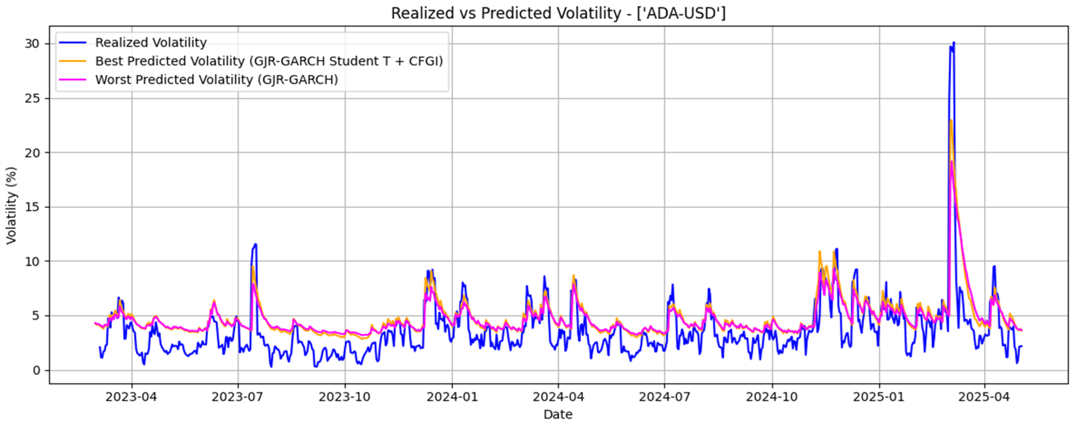
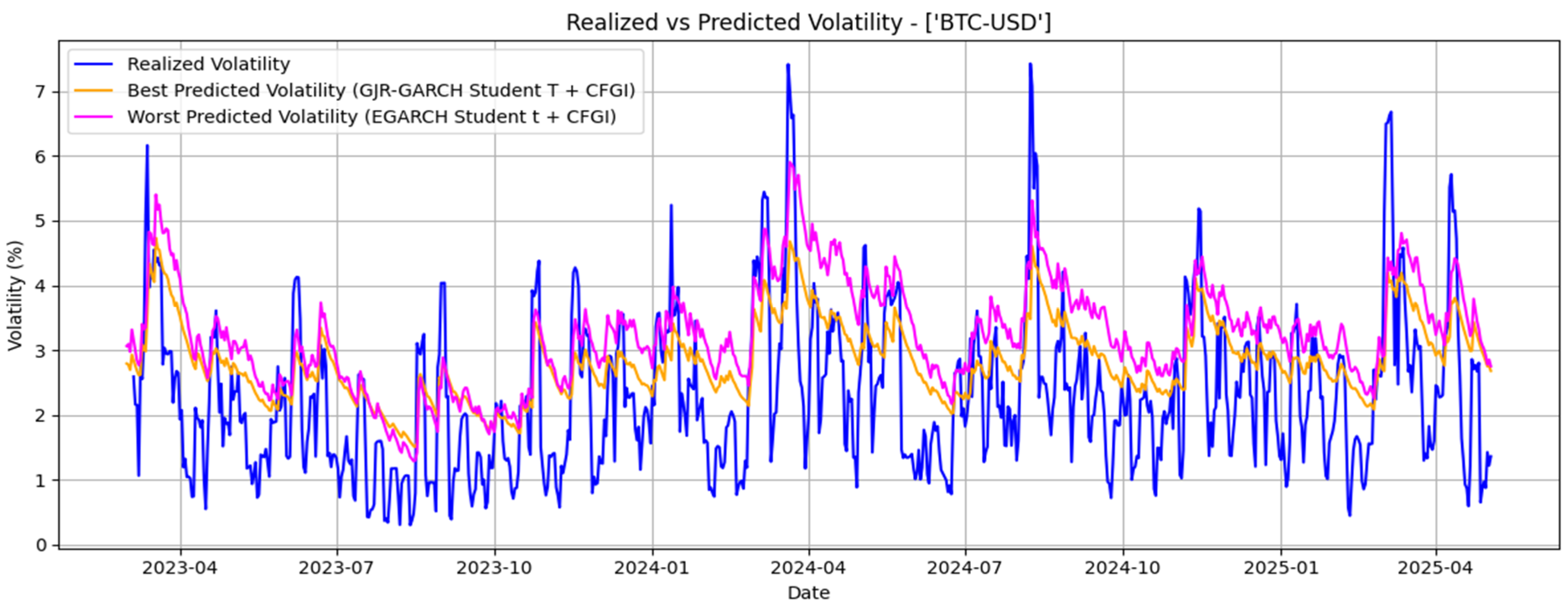
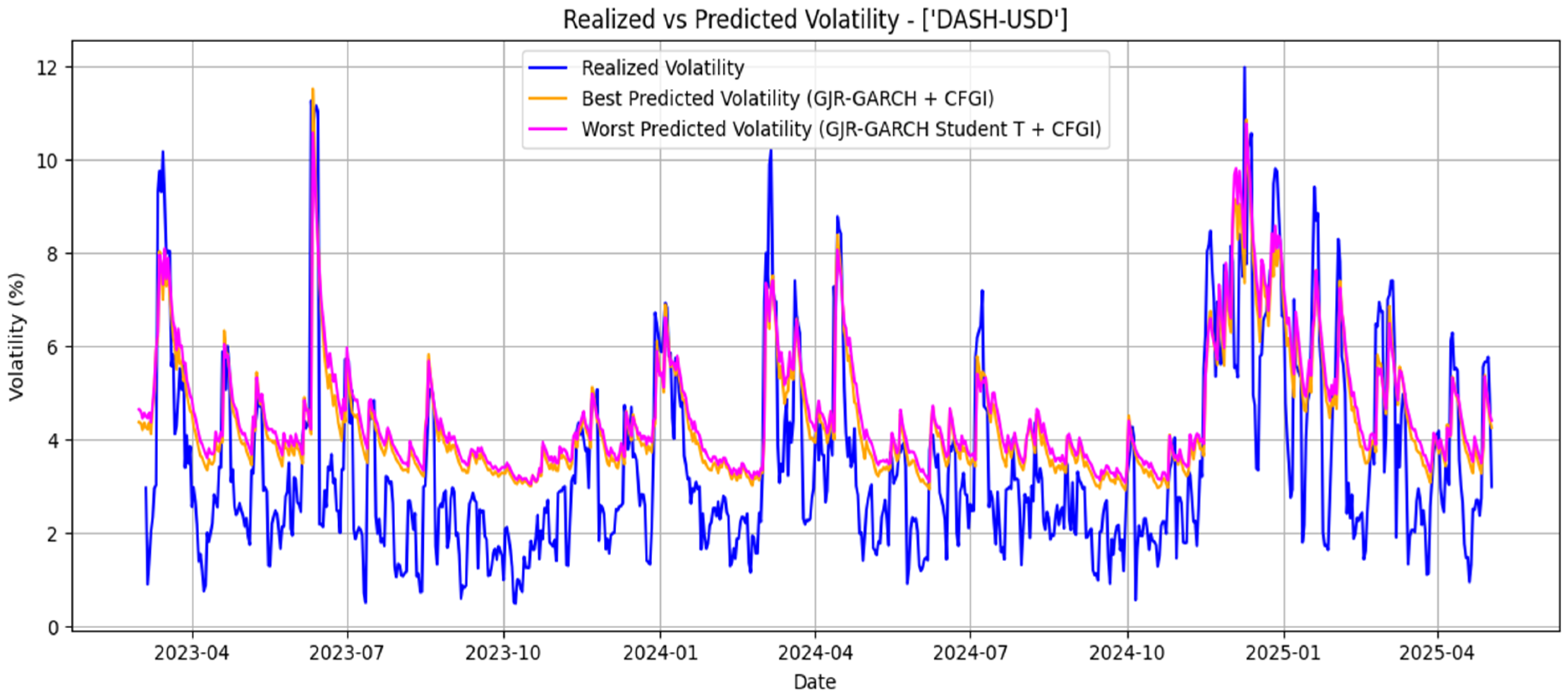
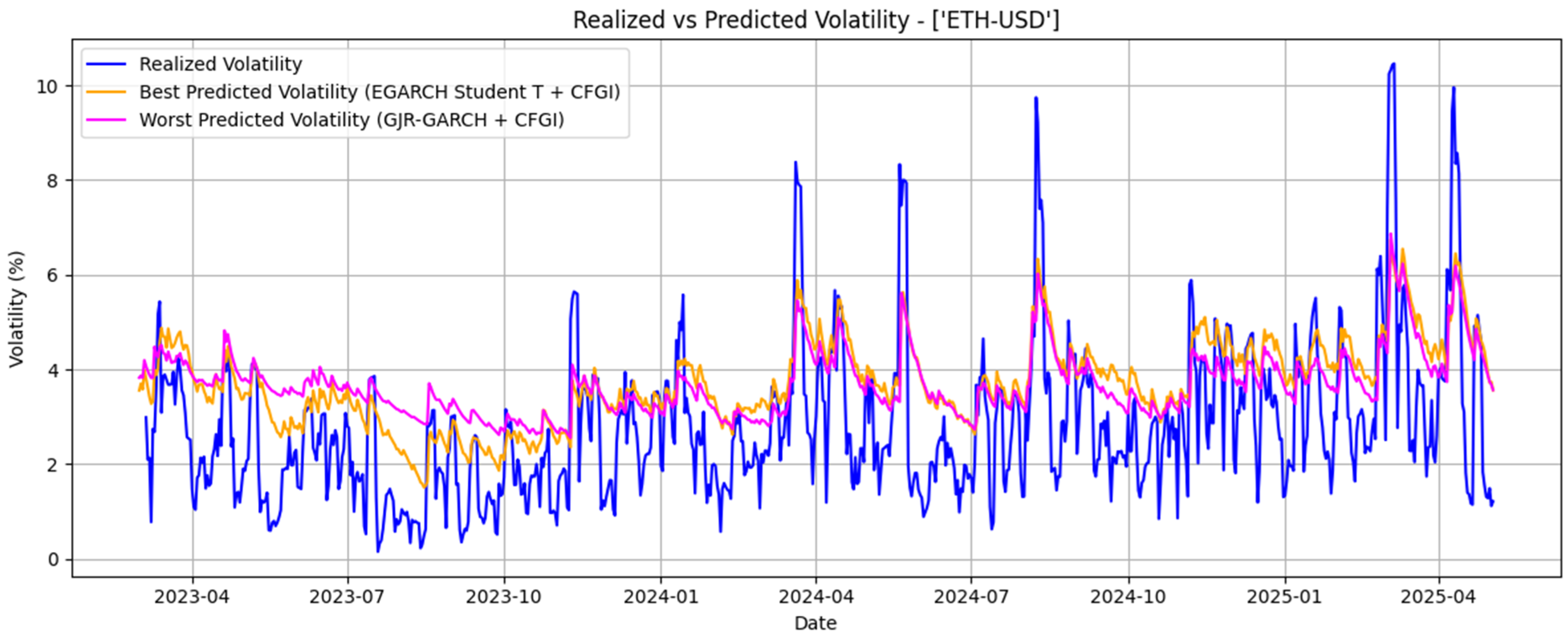
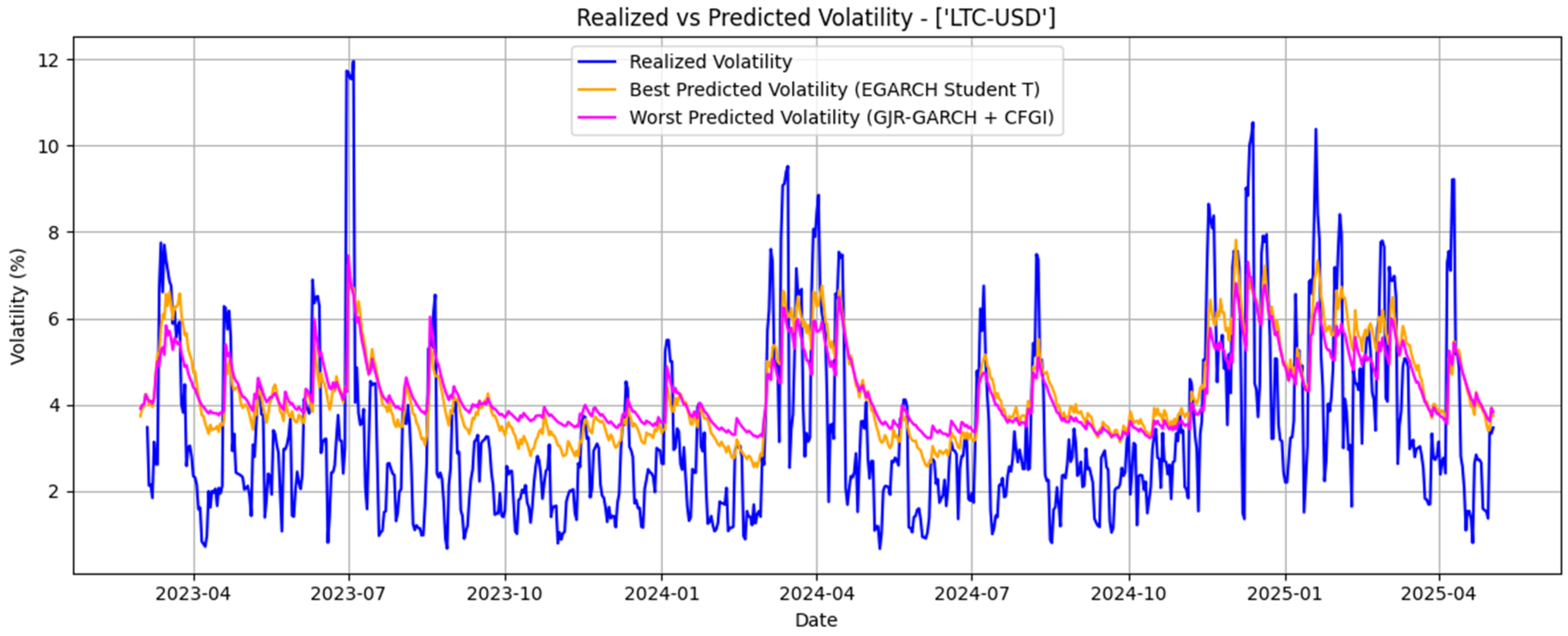
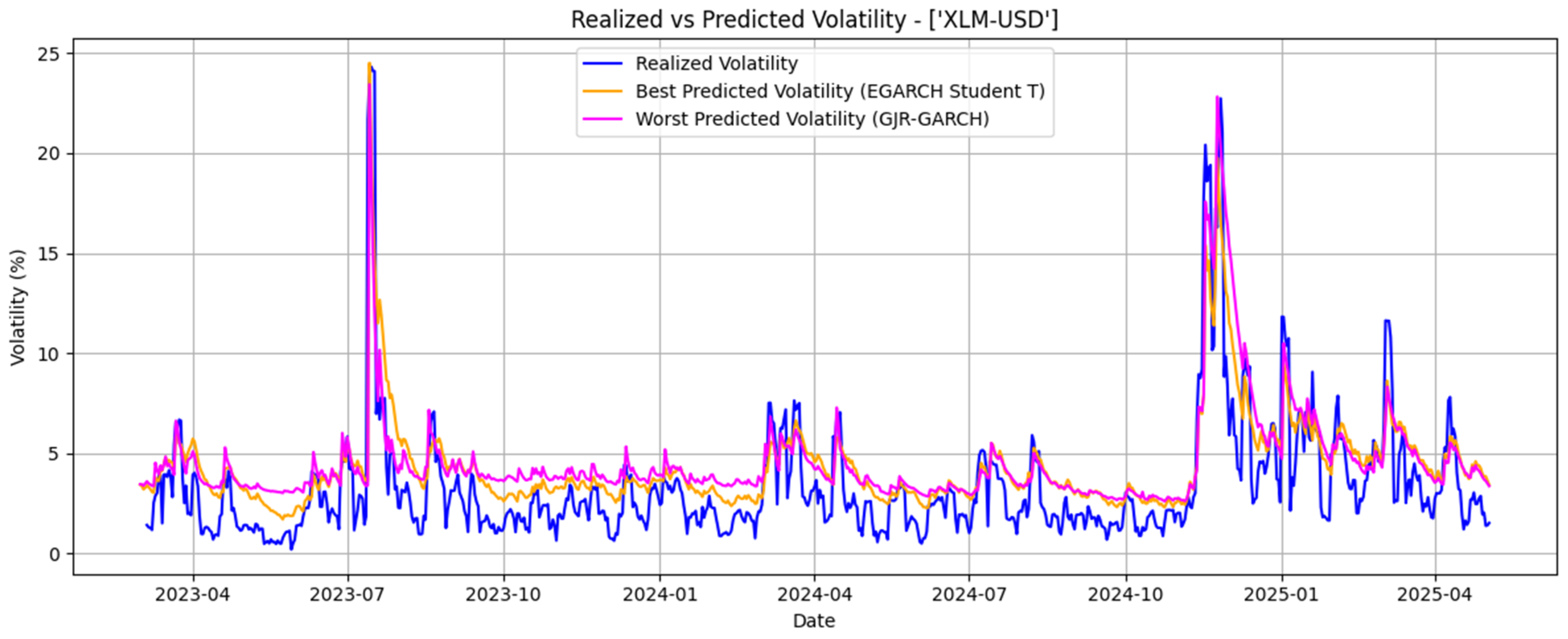
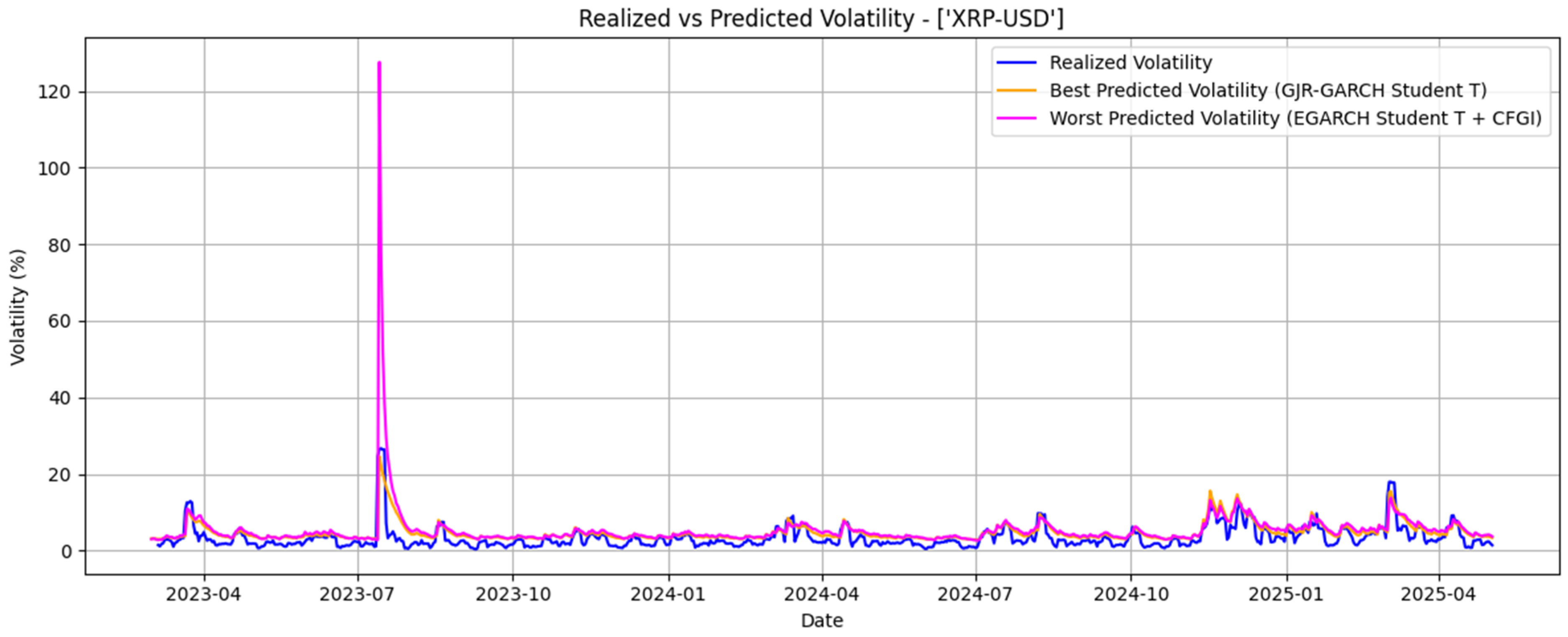
The hit rate is defined as the proportion of observations in the test set for which the model correctly predicts the direction of change in realized volatility. A value above 0.5 indicates directional accuracy exceeding a naive random benchmark. The results show that the hit rate consistently exceeds 0.5 across all models and cryptocurrency combinations, except for certain BTC (Figure 2) model specifications. This indicates that the models predict the correct direction of volatility change more frequently than a naive random benchmark, though we note this is a descriptive observation and no formal statistical test of directional accuracy has been conducted. Moreover, the correlation between forecasted and realized volatility is consistently high, with most models resulting in correlation coefficients above 0.75 (Figure 1, Figure 2, Figure 3, Figure 4, Figure 5, Figure 6 and Figure 7 presented below). In particular, the ADA (Figure 1), DASH (Figure 3), XLM (Figure 6), and GJR-GARCH models of XRP (Figure 7), we also observe values exceeding 0.8. These high correlations imply that the models effectively predict the magnitude of volatility movements and follow the overall trend and dynamics of realized volatility. On the other hand, ETH (Figure 4) and the EGARCH models for XRP (Figure 7) performed worse in the correlation test, with coefficients below 0.7. These findings show that the models not only provide statistically sound estimates but also offer valuable asset-specific insights in highly volatile environments, such as the crypto market.

5. Conclusions

The methodological basis employed in this research facilitated an extensive examination of cryptocurrency market volatility dynamics, using asymmetric GARCH-family models applied to seven significant, decentralized assets.

Volatility asymmetry was estimated using the γ parameter in both GJR-GARCH and EGARCH models. While the EGARCH model permits persistent asymmetry and the GJR-GARCH model accommodates directional shocks using a threshold mechanism, neither model resulted in statistically significant results for the selected cryptocurrencies in this study. Most of the γ coefficient followed the asymmetry assumption that negative shocks have a greater impact on volatility than positive shocks. Specific Student-t distribution models follow the asymmetry assumption that positive shocks have a greater impact on volatility than negative shocks, with the notable exception of XRP.

The addition of the CFGI as an exogenous dummy variable, activated at the 80th percentile to capture sentiment-induced regime changes, resulted in small but frequent performance improvements across numerous cryptocurrencies. Overall, the CFGI coefficient was not statistically significant in the conditional variance model across most specifications. While its inclusion produced marginal improvements in-sample and out-of-sample metrics for some assets, this should be interpreted cautiously, as it does not reflect a robust structural effect on conditional volatility dynamics.

Another observed pattern was the presence of the negative AR(1) coefficients in the conditional mean equation of all the cryptocurrencies, signaling the short-term mean balancing and reversal of daily returns. Additionally, the β_1 coefficient, which captures volatility persistence, was consistently above 0.7, indicating that once volatility rises, it remains elevated for a prolonged period.

Specifically, the EGARCH Student-t and GJR-GARCH Student-t models generally produced lower error values in out-of-sample exercises, particularly when using the QLIKE loss function to evaluate volatility forecasts. The directional performance metric also supports the models’ effectiveness in forecasting volatility, with the hit rate consistently above 0.5, indicating that the models have a better-than-random chance of predicting volatility direction. Moreover, the correlation coefficient between forecasted and realized volatility was typically above 0.7. It even exceeded 0.8 for specific cryptocurrencies, indicating that the models accurately tracked the overall movement and magnitude of volatility.

In conclusion, Hypothesis I is largely unsupported, Hypothesis II is only partly supported through Student-t innovations, and Hypothesis III is not convincingly supported. The findings are consistent across several statistical and practical criteria for model evaluation, reflecting the value of asymmetry-aware models that account for the statistical properties of returns and market behavior. These insights are not only academically relevant for future research but also valuable for risk management, derivative pricing, and volatility-based trading strategies in digital asset markets.

The empirical results suggest that GARCH-family models incorporating Student-t distributions tend to perform better across specifications, while leverage effects are found to be weak and heterogeneous across the seven cryptocurrencies examined. This is consistent with the distributional characteristics of cryptocurrency returns, which feature fat tails, excess kurtosis, and a propensity for extreme events.

The asymmetry terms in both EGARCH and GJR-GARCH specifications were largely statistically insignificant, providing only weak and heterogeneous evidence of leverage effects across the sample. These results suggest that asymmetric volatility dynamics are less pronounced in decentralized cryptocurrency markets than in traditional equity markets, and that caution is warranted in generalizing leverage-based interpretations to this asset class.

Additionally, the use of CFGI as a dummy variable to indicate high-greed market sentiment was not statistically significant across multi-asset scales. However, its inclusion proved beneficial in the out-of-sample testing phase of this research, with models that included it outperforming the baseline models for most cryptocurrencies. This supports the argument that investor sentiment and market mood play a particular role in volatility behavior in the cryptocurrency market.

6. Limitations and Future Research

This study has several limitations, including its confinement to seven decentralized cryptocurrencies and a sample period bounded by the availability of the CFGI, which may limit the generalizability of the findings. Additionally, the GARCH(1,1) structure may not fully capture long-memory dynamics, and the CFGI dummy variable did not yield statistically significant effects across most specifications, suggesting that alternative sentiment proxies may be worth exploring. Future research could extend this work by applying Markov-switching GARCH models to examine endogenous regime transitions more directly, or by incorporating hybrid deep learning architectures such as EGARCH-LSTM to improve out-of-sample forecasting accuracy.

References

1. Akin, I., Akin, M., Ozturk, Z., Hameed, A., Opara, V., & Satiroglu, H. (2024). Exploring fluctuations and interconnected movements in stock, commodity, and cryptocurrency markets. British Actuarial Journal, 29, e13. [Google Scholar] [CrossRef]
2. Akin, I., Khan, M. Z., Hameed, A., Chebbi, K., & Satiroglu, H. (2023). The ripple effects of CBDC-related news on Bitcoin returns: Insights from the DCC-GARCH model. Research in International Business and Finance, 66, 102060. [Google Scholar] [CrossRef]
3. Alternative.me. (2025). Crypto fear & greed index. Available online: https://alternative.me/crypto/fear-and-greed-index/ (accessed on 1 January 2025).
4. Barjašić, A., & Antulov-Fantulin, N. (2021). Time-varying volatility in Bitcoin market and information flow at minute-level frequency. Frontiers in Physics, 9, 644102. [Google Scholar] [CrossRef]
5. Benhamed, A., Messai, A., & El Montasser, G. (2023). On the determinants of Bitcoin returns and volatility: What we get from Gets? Sustainability, 15(3), 1761. [Google Scholar] [CrossRef]
6. Bhatnagar, M., Taneja, S., & Rupeika-Apoga, R. (2023). Demystifying the effect of the news (shocks) on crypto market volatility. Journal of Risk and Financial Management, 16(2), 136. [Google Scholar] [CrossRef]
7. Bollerslev, T. (1986). Generalized autoregressive conditional heteroskedasticity. Journal of Econometrics, 31(3), 307–327. [Google Scholar] [CrossRef]
8. Caporale, G. M., & Zekokh, T. (2018). Modelling volatility of cryptocurrencies using Markov-Switching GARCH models. Research in International Business and Finance, 48, 143–155. [Google Scholar] [CrossRef]
9. Chowdhury, A. (2016). Is Bitcoin the “Paris Hilton” of the currency world? Or are the early investors onto something that will make them rich? The Journal of Investing, 25(1), 64–72. [Google Scholar] [CrossRef]
10. da Silva, L., & Maciel, L. (2022). Forecasting volatility of cryptocurrencies: The role of GARCH-family models. Available online: https://anpad.com.br/uploads/articles/120/approved/9379c23ac12dc94053207373040bc791.pdf (accessed on 1 February 2025).
11. Ding, Z., Gosal, K., & McMurran, G. (2024). Bitcoin and Ethereum volatility forecasting with GARCH models. SSRN. [Google Scholar] [CrossRef]
12. Engle, R. F. (1982). Autoregressive conditional heteroscedasticity with estimates of the variance of United Kingdom inflation. Econometrica, 50(4), 987–1007. [Google Scholar] [CrossRef]
13. Engle, R. F. (2001). GARCH 101: The use of ARCH/GARCH models in applied econometrics. Journal of Economic Perspectives, 15(4), 157–168. [Google Scholar] [CrossRef]
14. Engle, R. F. (2002). New frontiers for ARCH models. Journal of Applied Econometrics, 17(5), 425–446. [Google Scholar] [CrossRef]
15. Fakhfekh, M., & Jeribi, A. (2020). Volatility dynamics of cryptocurrencies’ returns: Evidence from asymmetric and long memory GARCH models. Research in International Business and Finance, 51, 101075. [Google Scholar] [CrossRef]
16. Glosten, L. R., Jagannathan, R., & Runkle, D. E. (1993). On the relation between the expected value and the volatility of the nominal excess return on stocks. The Journal of Finance, 48(5), 1779–1801. [Google Scholar] [CrossRef]
17. Hansen, P. R., & Lunde, A. (2005). A forecast comparison of volatility models: Does anything beat a GARCH(1,1)? Journal of Applied Econometrics, 20(7), 873–889. [Google Scholar] [CrossRef]
18. Hyndman, R. J., & Athanasopoulos, G. (2018). Forecasting: Principles and practice (2nd ed.). OTexts. Available online: https://otexts.org/fpp2/ (accessed on 1 March 2025).
19. Ibrahim, B. A., Elamer, A. A., Alasker, T. H., Mohamed, M., & Abdou, H. (2024). Volatility contagion between cryptocurrencies, gold and stock markets pre-and-during COVID-19: Evidence using DCC-GARCH and cascade-correlation network. Financial Innovation, 10(1), 104. [Google Scholar] [CrossRef]
20. Kaplanov, N. (2012). Nerdy money: Bitcoin, the private digital currency, and the case against its regulation. Loyola Consumer Law Review, 25, 111. Available online: https://lawecommons.luc.edu/cgi/viewcontent.cgi?article=1920&context=lclr (accessed on 3 April 2025). [CrossRef]
21. Kim, Y., Jun, J., & Lee, H. (2021). Forecasting the volatility of the cryptocurrency market by GARCH and stochastic volatility. Mathematics, 9(14), 1614. [Google Scholar] [CrossRef]
22. Köse, T., Gür, T. H., & Ünal, U. (2025). Deep learning and machine learning insights into the global economic drivers of the Bitcoin price. Journal of Forecasting, 44, 1666–1698. [Google Scholar] [CrossRef]
23. Kristoufek, L. (2013). BitCoin meets Google trends and Wikipedia: Quantifying the relationship between phenomena of the Internet era. Scientific Reports, 3(1), 3415. [Google Scholar] [CrossRef]
24. Kufo, A., Gjeci, A., & Pilkati, A. (2024). Unveiling the influencing factors of cryptocurrency return volatility. Journal of Risk and Financial Management, 17(1), 12. [Google Scholar] [CrossRef]
25. Kyriazis, N. A., Daskalou, K., Arampatzis, M., Prassa, P., & Papaioannou, E. (2019). Estimating the volatility of cryptocurrencies during bearish markets by employing GARCH models. Heliyon, 5(8), e02239. [Google Scholar] [CrossRef]
26. Lo, A. W., & MacKinlay, A. C. (1988). Stock market prices do not follow random walks: Evidence from a simple specification test. The Review of Financial Studies, 1(1), 41–66. Available online: http://www.jstor.org/stable/2962126 (accessed on 6 April 2025). [CrossRef]
27. Naimy, V., Haddad, O., Fernández-Avilés, G., & El Khoury, R. (2021). The predictive capacity of GARCH-type models in measuring the volatility of crypto and world currencies. PLoS ONE, 16(1), e0247764. [Google Scholar] [CrossRef] [PubMed]
28. Naimy, V. Y., & Hayek, M. R. (2018). Modelling and predicting the Bitcoin volatility using GARCH models. International Journal of Mathematical Modelling and Numerical Optimization, 8(3), 197. [Google Scholar] [CrossRef]
29. Nelson, D. B. (1991). Conditional heteroskedasticity in asset returns: A new approach. Econometrica, 59(2), 347–370. [Google Scholar] [CrossRef]
30. Roy, D., Dubey, A., & Tiwary, D. (2024). Conceptualizing an institutional framework to mitigate crypto-assets’ operational risk. Journal of Risk and Financial Management, 17(12), 550. [Google Scholar] [CrossRef]
31. Wu, J. (2010). Threshold GARCH model: Theory and application. Available online: https://www.semanticscholar.org/paper/Threshold-GARCH-Model%3A-Theory-and-Application-Wu/25354cce5b929f4ffea35af191ba7beaab293cfb (accessed on 6 March 2025).
32. Yahoo Finance. (2025). Cryptocurrencies: Prices, changes, trading volume & daily charts. Available online: https://finance.yahoo.com/markets/crypto/all/ (accessed on 7 April 2025).
33. Yalcin, Y., & Yucel, E. M. (2006). The day-of-the-week effect on stock-market volatility and return: Evidence from emerging markets. Czech Journal of Economics and Finance, 56(5–6), 258–277. Available online: https://journal.fsv.cuni.cz/storage/1057_x.pdf (accessed on 8 May 2025).
34. Zahid, M., Iqbal, F., & Koutmos, D. (2022). Forecasting Bitcoin volatility using hybrid GARCH models with machine learning. Risks, 10(12), 237. [Google Scholar] [CrossRef]
35. Zakoian, J.-M. (1994). Threshold heteroskedastic models. Journal of Economic Dynamics and Control, 18(5), 931–955. [Google Scholar] [CrossRef]
Figure 1. Realized vs. Predicted Volatility ADA.
Jrfm 19 00390 g001
Figure 2. Realized vs. Predicted Volatility BTC.
Jrfm 19 00390 g002
Figure 3. Realized vs. Predicted Volatility DASH.
Jrfm 19 00390 g003
Figure 4. Realized vs. Predicted Volatility ETH.
Jrfm 19 00390 g004
Figure 5. Realized vs. Predicted Volatility LTC.
Jrfm 19 00390 g005
Figure 6. Realized vs. Predicted Volatility XLM.
Jrfm 19 00390 g006
Figure 7. Realized vs. Predicted Volatility XRP.
Jrfm 19 00390 g007