Property Tax, Local Sales Tax and Business Activity in Nevada: A Spatial Analysis


Abstract
1. Introduction
2. Previous Studies
2.1. Property Taxes and Business Activity
2.2. Local Sales Taxes, Border Effects, and Business Activity
2.3. Multi-Tax Bundles and Local Fiscal Decisions
2.4. Spatial Interactions and Fiscal Spillovers
2.5. Synthesis and Motivation for the Current Study
3. Tax Rates, Data and Empirical Approach
3.1. Data
- (1)
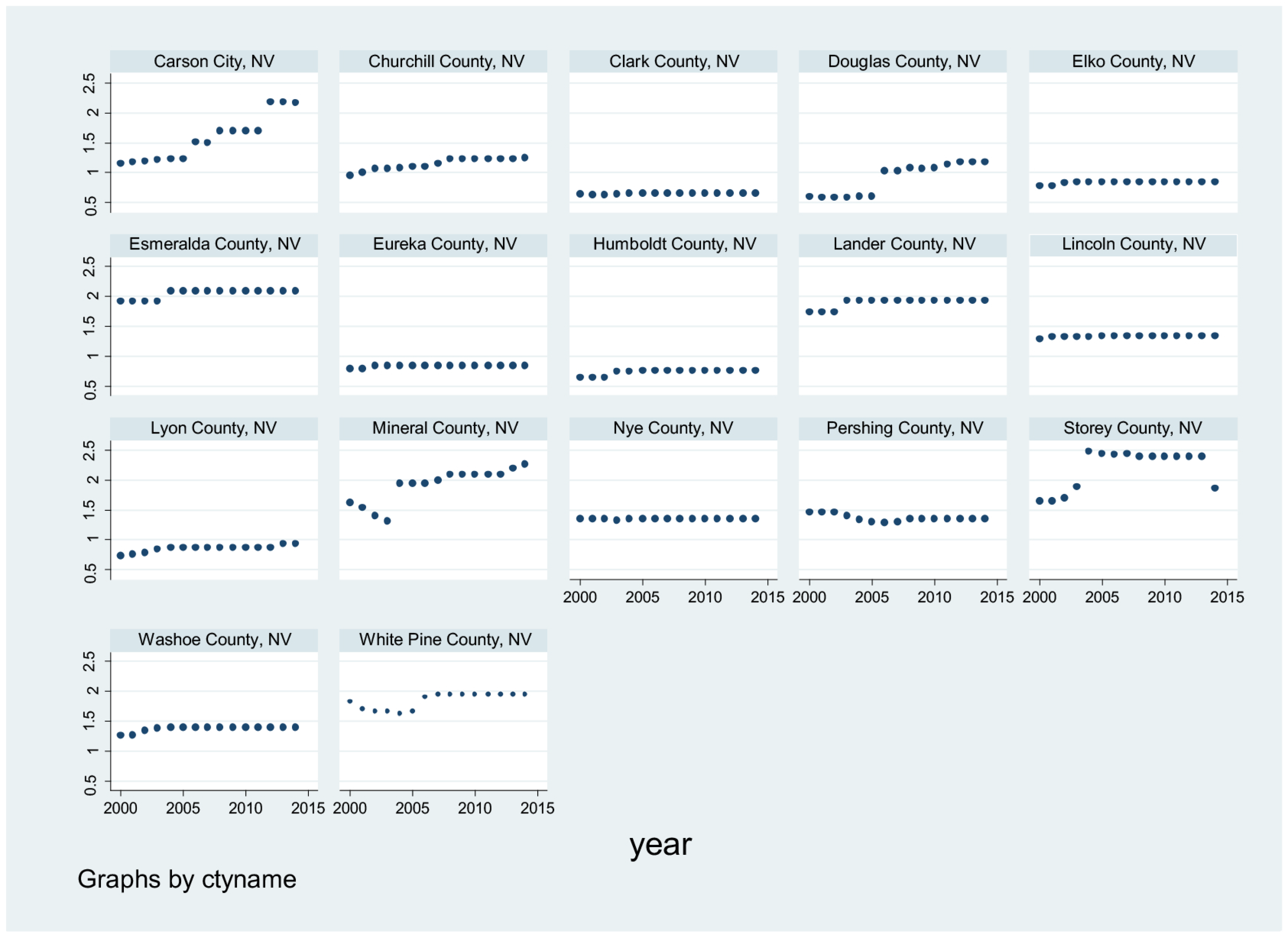
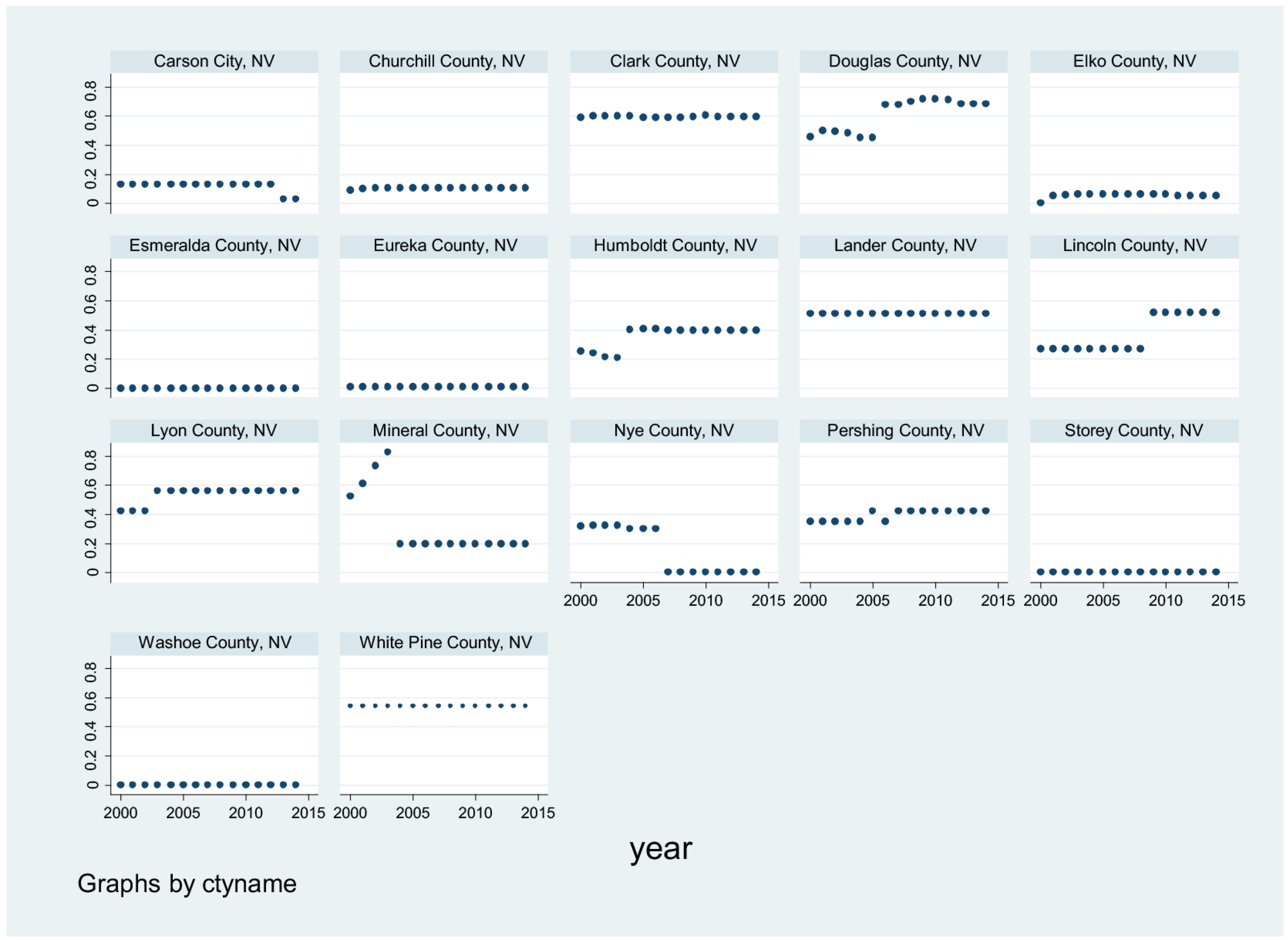
- Tax policy stability and changes post-2014: Nevada’s tax system changed materially after 2014, most notably with the introduction of the Commerce Tax in 2015, a gross receipts tax applying to businesses with annual revenues exceeding $4 million. This reform altered the effective tax bundle faced by firms, making it more difficult to isolate the effects of property and sales taxes on business activity in later years. By ending the sample in 2014, we focus on a period in which businesses were primarily exposed to property and sales taxes, thereby improving within-regime comparability.
- (2)
- Data availability and consistency: County-level business and public finance datasets are often released with delays and may undergo reporting or methodological changes over time. When this research began, post-2014 county-level series were not consistently available across sources, and extending the sample without accounting for potential measurement changes could introduce additional noise or bias.
- (3)
- Economic disruptions post-2014: The period after 2014 includes major events that could confound the relationship between local taxation and business activity, including federal tax reforms (e.g., the Tax Cuts and Jobs Act of 2017) and, later, the COVID-19 pandemic. These shocks introduced large economic fluctuations that may overshadow local fiscal effects, complicating interpretation.
3.2. Model Specification
4. Results
5. Robustness and Sensitivity Analyses
6. Discussion and Policy Implications
7. Summary and Conclusions
Author Contributions
Funding
Institutional Review Board Statement
Informed Consent Statement
Data Availability Statement
Conflicts of Interest
| 1 | See also (Zodrow, 2001) for a useful review on property tax incidence. |
| 2 | Mieszkowski builds on the general equilibrium model by (Harberger, 1962). |
| 3 | We attempted to compute Lagrange Multiplier (LM) diagnostics for spatial lag and spatial error dependence in selected cross-sections. In our small-N county setting and with year-specific estimation samples, some standard LM implementations return missing statistics due to numerical singularity or weight-list constraints after subsetting the spatial weights matrix. We therefore report Moran’s I on OLS residuals as a basic diagnostic and rely on the SDM’s theoretical appropriateness for cross-jurisdiction spillovers together with extensive robustness checks (alternative weight matrices and the Clark County exclusion) to assess sensitivity of the spatial specification. |
| 4 | Due to the inclusion of both county- and year-fixed effects, some variables (e.g., the share of the nonwhite population and the interaction between the school tax rate and the post-2005 dummy variable) are dropped from some specifications due to high multicollinearity. |
References
- Deller, S., & Maher, C. (2024). Do local fiscal decisions impact economic growth: The case of Wisconsin. State and Local Government Review, 56(3), 235–260. [Google Scholar] [CrossRef] [Scilit]
- Duranton, G., Gobillon, L., & Overman, H. (2011). Assessing the effects of local taxation using microgeographic data. The Economic Journal, 121(555), 1017–1046. [Google Scholar] [CrossRef] [Scilit]
- Elhorst, P. (2010). Applied spatial econometrics: Raising the bar. Spatial Economic Analysis, 5(1), 9–28. [Google Scholar] [CrossRef] [Scilit]
- Enami, A., Reynolds, L., & Rohlin, S. (2023). The effect of property taxes on businesses: Evidence from a dynamic regression discontinuity approach. Regional Science and Urban Economics, 100, 103895. [Google Scholar] [CrossRef] [Scilit]
- Fajgelbaum, P., & Gaubert, C. (2025). Optimal spatial policies (NBER Working Paper No. 33493). National Bureau of Economic Research. [Google Scholar]
- Feld, L., & Kirchgässner, G. (2003). The impact of corporate and personal income taxes on the location of firms and on employment: Some panel evidence for the Swiss cantons. Journal of Public Economics, 87(1), 129–155. [Google Scholar] [CrossRef] [Scilit]
- Fox, W. (1986). Tax structure and the location of economic activity along state borders. National Tax Journal, 39(4), 387–401. [Google Scholar] [CrossRef] [Scilit]
- Hamilton, B. (1975). Zoning and property taxation in a system of local governments. Urban Studies, 12(2), 205–211. [Google Scholar] [CrossRef] [Scilit]
- Hamilton, B. (1976). The effects of property taxes and local public spending on property values: A theoretical comment. Journal of Political Economy, 84(3), 647–650. [Google Scholar] [CrossRef] [Scilit]
- Harberger, A. (1962). The incidence of the corporation income tax. Journal of Political Economy, 70(3), 215–240. [Google Scholar] [CrossRef] [Scilit]
- Hoyt, W., & Harden, W. (2005). MSA location and the impact of state taxes on employment and population: A comparison of border and interior MSA’s (Working Paper, 1). Institute for Federalism and Intergovernmental Relations. [Google Scholar]
- Kenyon, D., Langley, A., & Paquin, B. (2012). Rethinking property tax incentives for business. Lincoln Institute of Land Policy. [Google Scholar]
- LeSage, J., & Pace, K. (2009). Introduction to spatial econometrics. Chapman and Hall/CRC. [Google Scholar]
- Mieszkowski, P. (1970). The property tax: An excise tax or a profits tax? Journal of Public Economics, 1(1), 73–96. [Google Scholar] [CrossRef] [Scilit]
- Mieszkowski, P., & Zodrow, G. (1989). Taxation and the Tiebout model: The differential effects of head taxes, taxes on land rents, and property taxes. Journal of Economic Literature, 27(3), 1098–1146. [Google Scholar]
- Muthitacharoen, A., & Zodrow, G. (2012). Revisiting the excise tax effects of the property tax. Public Finance Review, 40(5), 555–583. [Google Scholar] [CrossRef] [Scilit]
- Netzer, D. (1966). Economics of the property tax. The Brooklyn Institute. [Google Scholar]
- Rohlin, S., Rosenthal, S., & Ross, A. (2014). Tax avoidance and business location in a state border model. Journal of Urban Economics, 83, 34–49. [Google Scholar] [CrossRef] [Scilit]
- Rohlin, S., & Thompson, J. (2018). Local sales taxes, employment, and tax competition. Regional Science and Urban Economics, 70, 373–383. [Google Scholar] [CrossRef] [Scilit]
- Shon, J. (2017). State-local sales tax, spillover, and economic activity: Examining county governments in the U.S. Local Government Studies, 43(3), 429–450. [Google Scholar] [CrossRef] [Scilit]
- Simon, H. (1943). The incidence of a tax on urban real property. The Quarterly Journal of Economics, 57(3), 398–420. [Google Scholar] [CrossRef] [Scilit]
- Snodgrass, D. W., & Otto, D. (1990). Analysis of local sales taxation in rural areas: An Oklahoma case study. Growth and Change, 21(2), 34–45. [Google Scholar] [CrossRef] [Scilit]
- Thompson, J., & Rohlin, S. (2012). The effect of sales taxes on employment: New evidence from cross-border panel data analysis. National Tax Journal, 65(4), 1023–1041. [Google Scholar] [CrossRef] [Scilit]
- Tosun, M., & Skidmore, M. (2007). Cross-border shopping and the sales tax: An examination of food purchases in West Virginia. The BE Journal of Economic Analysis & Policy, 7(1), 1–20. [Google Scholar]
- Walsh, M., & Jones, J. (1988). More evidence on the “border tax” effect: The case of West Virginia, 1979-84. National Tax Journal, 41(2), 261–265. [Google Scholar] [CrossRef] [Scilit]
- Wassmer, R. (1993). Property taxation, property base, and property value: An empirical test of the “new view”. National Tax Journal, 46(2), 135–159. [Google Scholar] [CrossRef] [Scilit]
- Wildasin, D. (1989). Interjurisdictional capital mobility: Fiscal externality and a corrective subsidy. Journal of Urban Economics, 25(2), 193–212. [Google Scholar] [CrossRef] [Scilit]
- Zodrow, G. (2001). The property tax as a capital tax: A room with three views. National Tax Journal, 54(1), 139–156. [Google Scholar] [CrossRef] [Scilit]
- Zodrow, G., & Mieszkowski, P. (1986). The new view of the property tax: A reformulation. Regional Science and Urban Economics, 16(3), 309–327. [Google Scholar] [CrossRef] [Scilit]



| Variable | Mean | Std. Dev. | Min | Max |
|---|---|---|---|---|
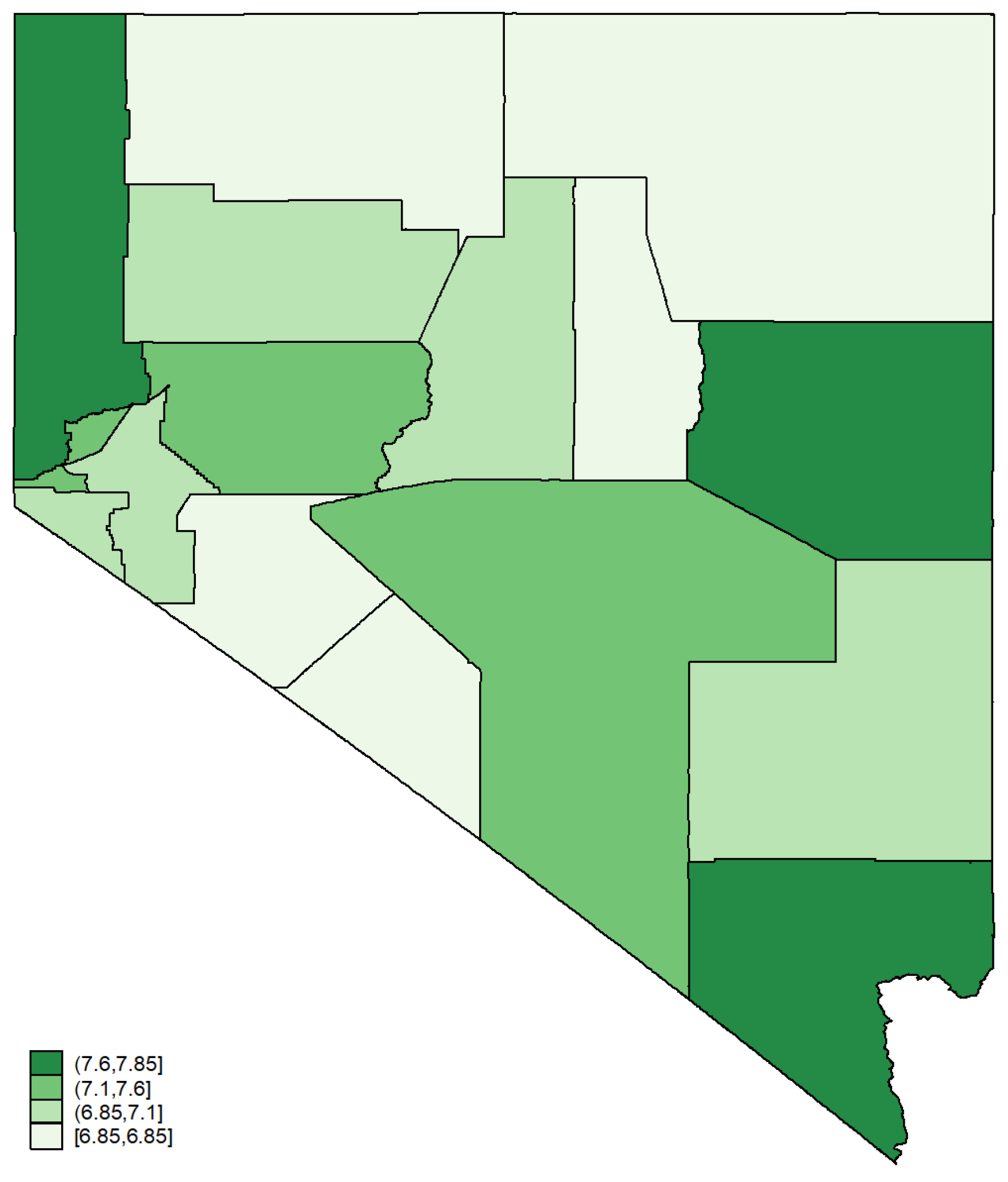
| Combined state and local sales tax rate | 7.166176 | 0.324478 | 6.85 | 7.85 |
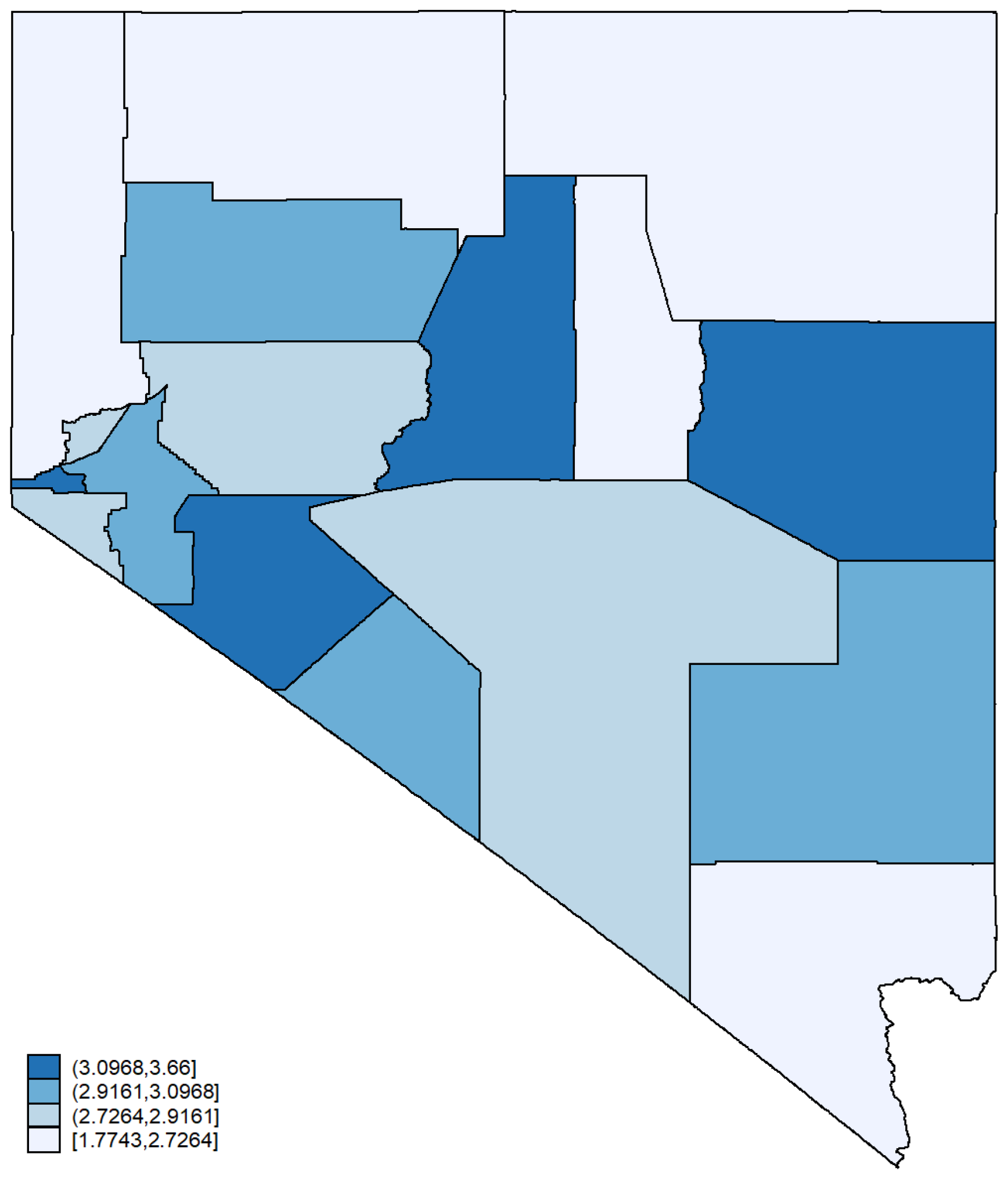
| Total county property tax rate | 2.875937 | 0.487646 | 1.6973 | 3.66 |
| Total county property tax rate components: | ||||
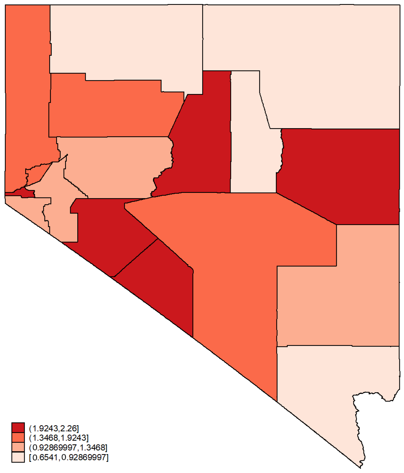
| County property tax rate | 1.340889 | 0.511047 | 0.579 | 2.469 |
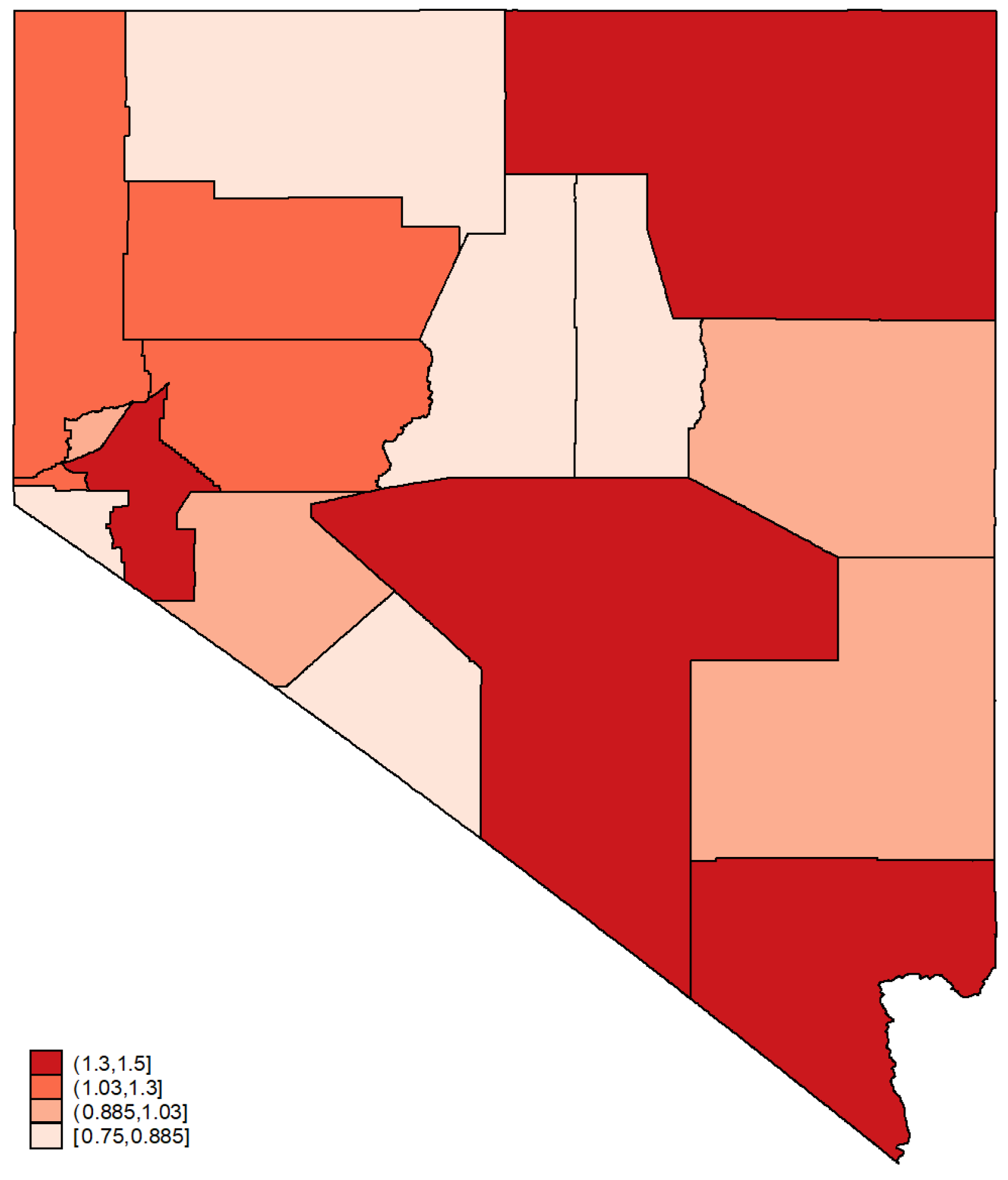
| School tax rate | 1.094453 | 0.234126 | 0.75 | 1.5 |
| County combined special district | 0.274582 | 0.238466 | 0 | 0.826 |
| Employment | 60,241.94 | 178,697.8 | 0 | 865,940 |
| Annual payroll | 2,163,629 | 6,455,486 | 0 | 3.26 × 10⁷ |
| Per capita income | 32,459.5 | 8091.901 | 16,280 | 56,469 |
| Number of establishments (total) | 3368.392 | 9078.762 | 10 | 42,031 |
| Number of establishments (1–9 employees) | 2436.016 | 6472.133 | 8 | 30,051 |
| Number of establishments (10–49 employees) | 743.902 | 2054.76 | 1 | 9528 |
| Share of population (age 20–64) | 0.58793 | 0.03306 | 0.506915 | 0.668267 |
| Share of population (age 65+) | 0.151582 | 0.049366 | 0.059978 | 0.278487 |
| Share of nonwhite population | 0.112072 | 0.064222 | 0.04058 | 0.442975 |
| #. Obs. | 255 | |||
| State | Sales Tax Rate (Highest Combined State and Local Rate, 2014) | Average Effective Property Tax Rate, 2013 |
|---|---|---|
| Alaska | 0% (7.5%) | 1.18% |
| Arizona | 5.6% (10.73%) | 0.84% |
| California | 7.5% (10%) | 0.81% |
| Colorado | 2.9% (10%) | 0.60% |
| Hawaii | 4.0% (4.5%) | 0.27% |
| Idaho | 6% (9%) | 0.76% |
| Montana | 0% | 0.85% |
| Nevada | 6.85% (7.85%) | 0.85% |
| New Mexico | 5.1% (8.69%) | 0.74% |
| Oregon | 0% | 1.08% |
| Utah | 6.0% (8.05%) | 0.68% |
| Washington | 6.5% (9.6%) | 1.08% |
| Wyoming | 4.0% (6%) | 0.61% |
| Outcome | Weight Matrix | p | |
|---|---|---|---|
| Employment | M (inverse-distance) | 0.0954 | 0.7574 |
| W (contiguity) | 0.0295 | 0.8636 | |
| Annual payroll | M | 0.0715 | 0.7891 |
| W | 0.0290 | 0.8648 | |
| Establishments | M | 0.4274 | 0.5133 |
| W | 0.0553 | 0.8141 | |
| Estab. 1–9 | M | 0.4541 | 0.5004 |
| W | 0.0397 | 0.8421 | |
| Estab. 10–49 | M | 0.4176 | 0.5181 |
| W | 0.6795 | 0.4097 |
| Employment | Payroll | Establishments | Estab. (1–9) | Estab. (10–49) | |||||||
|---|---|---|---|---|---|---|---|---|---|---|---|
| Non-IV | IV (Sales) | Non-IV | IV (Sales) | Non-IV | IV (Sales) | Non-IV | IV (Sales) | Non-IV | IV (Sales) | ||
| Direct | Total property tax rate | 3569.2 | 1179.3 | 173,335.4 | 2949.1 | 153.5 | −37.46 | 89.45 | −56.23 | 46.26 | 15.09 |
| (4689.5) | (4944.0) | (218,792.2) | (229,458.7) | (133.1) | (137.8) | (91.43) | (95.35) | (36.61) | (37.72) | ||
| Total sales tax rate | −914.5 | −372,131.0 ** | −4810.0 | −17,009,417.8 ** | −129.4 | −13,430.7 *** | −117.4 | −9264.7 *** | −5.341 | −2812.7 ** | |
| (7995.1) | (155,136.2) | (373,525.4) | (7,206,895.6) | (228.7) | (4328.0) | (158.8) | (3000.5) | (61.88) | (1183.7) | ||
| Per capita income | −0.366 * | 0.729 * | −16.29 * | 33.50 | −0.0113 ** | 0.0258 ** | −0.00728 ** | 0.0176 ** | −0.00263 * | 0.00571 * | |
| (0.187) | (0.438) | (8.726) | (20.38) | (0.00532) | (0.0122) | (0.00366) | (0.00851) | (0.00145) | (0.00334) | ||
| Age 20∼64 | 158,807.0 * | −62,712.5 | 4,890,639.5 | −4,707,311.6 | 2321.2 | −5774.3 * | 981.2 | −4819.7 ** | 880.8 | −667.2 | |
| (83,139.2) | (124,520.6) | (3,883,014.1) | (5,800,260.7) | (2370.6) | (3499.7) | (1637.7) | (2425.0) | (646.4) | (956.0) | ||
| Age 65+ | 131,607.9 * | −294,261.3 | 4,077,008.7 | −15,490,752.2 * | 1979.9 | −13,880.4 *** | 751.0 | −10,323.7 *** | 829.0 | −2405.7 * | |
| (74,777.5) | (189,228.2) | (3,489,718.4) | (8,788,716.4) | (2128.6) | (5279.2) | (1467.3) | (3650.0) | (581.9) | (1448.9) | ||
| Indirect | Total property tax rate | 11,305.8 | 27,962.3 *** | 456,820.6 | 1,148,232.0 *** | 306.9 | 700.6 *** | 256.0 * | 476.3 *** | 17.22 | 127.1 ** |
| (7316.5) | (8217.8) | (341,640.3) | (382,230.3) | (212.3) | (231.2) | (149.3) | (163.1) | (55.99) | (61.21) | ||
| Total sales tax rate | 3180.1 | −114,404.9 | 374,145.6 | 7,242,487.8 | 319.1 | 12,425.1 * | 239.6 | 9122.5 * | 67.61 | 2770.6 | |
| (17,344.4) | (264,829.8) | (815,734.1) | (12,358,863.7) | (505.5) | (7494.0) | (358.6) | (5311.7) | (132.6) | (1980.5) | ||
| Per capita income | −0.0668 | 0.249 | −8.649 | −17.44 | −0.0117 | −0.0348 | −0.00885 | −0.0249 | −0.00236 | −0.00816 | |
| (0.351) | (0.790) | (16.44) | (36.96) | (0.0102) | (0.0224) | (0.00722) | (0.0159) | (0.00269) | (0.00590) | ||
| Age 20∼64 | 108,190.7 | 503,561.6 * | 3,726,931.9 | 32,550,313.2 *** | 1868.4 | 26,388.0 *** | 1191.6 | 15,839.4 *** | 410.0 | 7783.6 *** | |
| (96,239.6) | (267,644.2) | (4,409,450.2) | (12,585,571.0) | (2731.0) | (7677.9) | (1914.0) | (5432.2) | (720.2) | (2036.4) | ||
| Age 65+ | −65,407.9 | 226,049.0 | −3,485,292.7 | 22,884,443.7 | −2552.2 | 24,454.1 *** | −1851.8 | 15,730.1 ** | −513.4 | 6670.7 *** | |
| (79,879.4) | (329,023.3) | (3,717,130.0) | (15,395,679.0) | (2293.1) | (9340.7) | (1617.0) | (6607.3) | (609.9) | (2480.7) | ||
| nonwhite | 46,970.0 | 136,208.2 | 2,091,486.4 | 3,278,237.9 | 1927.6 | 1162.8 | 1379.0 | 179.4 | 361.1 | 620.0 | |
| (56,609.3) | (88,159.0) | (2,652,031.6) | (4,108,356.1) | (1648.1) | (2491.1) | (1163.8) | (1761.7) | (435.1) | (660.5) | ||
| Total | Total property tax rate | 14,874.9 ** | 29,141.6 *** | 630,155.9 ** | 1,151,181.1 *** | 460.4 ** | 663.2 *** | 345.4 ** | 420.1 ** | 63.48 | 142.2 ** |
| (6768.4) | (8037.8) | (316,498.2) | (375,402.2) | (198.6) | (229.1) | (142.1) | (163.7) | (51.06) | (59.11) | ||
| Total sales tax rate | 2265.5 | −486,535.9 * | 369,335.7 | −9,766,930.0 | 189.6 | −1005.5 | 122.2 | −142.2 | 62.27 | −42.09 | |
| (20,811.0) | (275,553.7) | (978,633.3) | (12,918,255.1) | (608.2) | (7886.3) | (433.2) | (5657.5) | (158.6) | (2043.4) | ||
| Per capita income | −0.433 | 0.978 | −24.94 | 16.07 | −0.0230 ** | −0.00892 | −0.0161 ** | −0.00738 | −0.00499 * | −0.00245 | |
| (0.364) | (0.865) | (17.09) | (40.64) | (0.0107) | (0.0248) | (0.00762) | (0.0178) | (0.00277) | (0.00643) | ||
| Age 20∼64 | 266,997.7 ** | 440,849.2 | 8,617,571.4 | 27,843,001.6 ** | 4189.6 | 20,613.7 ** | 2172.8 | 11,019.8 * | 1290.9 | 7116.4 *** | |
| (127,655.8) | (287,948.0) | (5,912,170.7) | (13,616,099.9) | (3674.3) | (8370.9) | (2607.1) | (5956.9) | (956.8) | (2196.3) | ||
| Age 65+ | 66,199.9 | −68,212.4 | 591,716.1 | 7,393,691.5 | −572.3 | 10,573.7 | −1100.8 | 5406.4 | 315.5 | 4265.0 * | |
| (100,370.1) | (316,254.1) | (4,703,000.4) | (14,894,446.3) | (2925.0) | (9121.4) | (2084.2) | (6536.1) | (763.1) | (2373.2) | ||
| nonwhite | −12,417.4 | 129,205.8 | −1,190,063.9 | 2,455,586.7 | −817.6 | 474.9 | −702.1 | −380.4 | −70.34 | 535.0 | |
| (58,670.5) | (85,428.6) | (2,753,780.0) | (3,993,751.8) | (1722.7) | (2439.0) | (1229.0) | (1746.3) | (447.3) | (632.9) | ||
| Employment | Payroll | Establishments | Estab. (1–9) | Estab. (10–49) | |||||||
|---|---|---|---|---|---|---|---|---|---|---|---|
| Non-IV | IV (Sales) | Non-IV | IV (Sales) | Non-IV | IV (Sales) | Non-IV | IV (Sales) | Non-IV | IV (Sales) | ||
| Direct | Combined special district rate | −562.9 | 19,593.1 * | −57,936.2 | 905,759.7 | −99.92 | 773.9 ** | −80.29 | 586.6 ** | −19.02 | 120.4 |
| (7556.1) | (11,810.4) | (353,940.7) | (551,364.0) | (210.9) | (322.8) | (147.7) | (227.9) | (56.86) | (86.74) | ||
| School tax rate | −26,025.9 * | −142,410.7 *** | −1,210,066.5 * | −7,162,189.0 *** | −925.7 ** | −6016.4 *** | −657.3 ** | −4316.9 *** | −183.1 * | −1184.2 *** | |
| (14,844.8) | (46,865.2) | (694,746.6) | (2,183,651.6) | (416.0) | (1270.8) | (293.3) | (888.6) | (109.5) | (350.6) | ||
| County tax rate | 6665.3 | −18,443.1 * | 281,580.2 | −1,015,867.9 ** | 122.4 | −974.2 *** | 12.03 | −767.6 *** | 83.89 * | −139.5 * | |
| (5835.3) | (11,117.6) | (273,243.3) | (517,793.2) | (162.1) | (300.8) | (112.8) | (209.0) | (44.47) | (83.98) | ||
| Total sales tax rate | −1144.3 | −420,046.5 ** | 6778.6 | −21,156,103.3 *** | −4.216 | −18,240.3 *** | 0.0730 | −13,244.0 *** | 6.574 | −3482.6 *** | |
| (8854.3) | (164,207.6) | (414,926.7) | (7,656,260.5) | (248.0) | (4462.0) | (174.9) | (3118.3) | (66.05) | (1229.8) | ||
| Indirect | Combined special district rate | 34,575.5 *** | 28,139.4 | 1,639,983.2 *** | 953,141.1 | 1018.7 *** | 701.8 | 729.6 *** | 721.7 | 156.8 * | −76.92 |
| (11,904.4) | (22,771.9) | (556,266.6) | (1,066,663.6) | (333.9) | (637.1) | (241.4) | (466.0) | (83.06) | (156.9) | ||
| School tax rate | −103,070.5 *** | −18,775.0 | −4,825,094.8 *** | 940,341.4 | −3134.2 *** | 691.3 | −2007.4 ** | −120.8 | −777.2 *** | 664.4 | |
| (38,369.7) | (89,409.4) | (1,792,237.5) | (4,181,644.8) | (1107.6) | (2496.2) | (799.8) | (1806.1) | (265.2) | (628.3) | ||
| County tax rate | 13,179.8 | 33,879.1 * | 627,980.6 | 1,960,686.5 ** | 529.2 * | 1476.9 *** | 368.8 * | 891.4 ** | 99.54 | 408.3 *** | |
| (10,332.2) | (18,301.7) | (483,863.7) | (856,632.8) | (290.5) | (505.7) | (208.2) | (362.0) | (74.90) | (131.7) | ||
| Total sales tax rate | 24,863.9 | 313,833.5 | 1,282,562.7 | 21,886,355.2 | 1105.0 * | 14,571.0 * | 793.3 * | 7071.5 | 257.5 * | 5541.7 ** | |
| (19,793.3) | (311,358.1) | (932,517.6) | (14,594,770.4) | (566.8) | (8653.7) | (412.1) | (6253.7) | (140.4) | (2204.8) | ||
| Total | Combined special district rate | 34,012.7 ** | 47,732.5 * | 1,582,047.0 ** | 1,858,900.8 | 918.8 ** | 1475.7 * | 649.3 ** | 1308.3 ** | 137.8 | 43.43 |
| (14,063.9) | (28,635.0) | (657,774.6) | (1,343,376.2) | (397.5) | (804.2) | (290.0) | (590.0) | (95.93) | (195.7) | ||
| School tax rate | −129,096.4 *** | −161,185.6 * | −6,035,161.3 *** | −6,221,847.6 | −4059.8 *** | −5325.2 ** | −2664.7 *** | −4437.7 ** | −960.3 *** | −519.8 | |
| (44,996.2) | (94,902.0) | (2,101,818.4) | (4,448,156.8) | (1300.6) | (2675.4) | (943.4) | (1964.2) | (306.3) | (646.2) | ||
| County tax rate | 19,845.1 ** | 15,436.0 | 909,560.9 ** | 944,818.6 | 651.6 ** | 502.7 | 380.8 * | 123.8 | 183.4 *** | 268.9 ** | |
| (9817.5) | (17,300.6) | (460,064.3) | (813,104.0) | (278.5) | (486.3) | (203.5) | (354.4) | (68.46) | (120.3) | ||
| Total sales tax rate | 23,719.6 | −106,212.9 | 1,289,341.2 | 730,251.8 | 1100.8 * | −3669.3 | 793.4 | −6172.5 | 264.1 | 2059.1 | |
| (23,175.0) | (340,348.1) | (1,091,859.7) | (15,996,957.2) | (666.3) | (9555.2) | (487.9) | (6980.7) | (161.7) | (2357.0) | ||
| Direct Effects | Indirect Effects | |||||||||
|---|---|---|---|---|---|---|---|---|---|---|
| Employment | Annual Payroll | Number of Establishments | Establishment Size: 1–9 | Establishment Size: 10–49 | Employment | Annual Payroll | Number of Establishments | Establishment Size: 1–9 | Establishment Size: 10–49 | |
| Combined special district rate | 6397.4 | 337,130.4 | 225.2 | 192.3 | 4.636 | 49,113.3 *** | 2,332,795.7 *** | 1592.9 *** | 1142.4 *** | 268.6 ** |
| (9169.7) | (425,162.2) | (249.7) | (173.6) | (71.10) | (15,904.3) | (737,409.2) | (435.8) | (311.7) | (114.3) | |
| School tax rate | −34,815.2 ** | −1,667,490.3 ** | −1188.1 *** | −824.1 *** | −246.2 ** | −92,651.5 ** | −4,211,203.9 ** | −3091.1 *** | −2057.9 ** | −727.6 ** |
| (15,072.0) | (697,407.1) | (412.3) | (288.0) | (115.3) | (41,716.4) | (1,929,421.9) | (1164.9) | (829.2) | (298.6) | |
| County tax rate | −2159.4 | −125,923.6 | −146.3 | −172.8 | 35.02 | 14,578.2 | 716,723.5 | 673.1 ** | 520.1 ** | 91.23 |
| (6111.9) | (283,012.4) | (165.8) | (114.8) | (47.96) | (11,452.0) | (531,330.3) | (312.1) | (221.6) | (85.01) | |
| Total sales tax rate | 12,231.7 | 799,756.6 * | 534.1 * | 421.7 ** | 64.46 | 33,614.1 | 1,759,567.5 | 1543.2 ** | 1235.6 *** | 238.1 |
| (10,248.7) | (475,668.5) | (279.6) | (195.6) | (78.67) | (23,036.0) | (1,078,384.8) | (643.1) | (464.2) | (166.2) | |
| Per capita income | −0.143 | −3.377 | −0.00366 | −0.00186 | −0.00133 | 0.325 | 19.67 | 0.00370 | 0.00505 | −0.00216 |
| (0.216) | (10.04) | (0.00588) | (0.00412) | (0.00165) | (0.482) | (22.47) | (0.0131) | (0.00943) | (0.00347) | |
| Age 20–64 | 237,470.2 ** | 9,592,985.5 * | 5872.4 ** | 3008.0 | 1959.9 ** | 1,170,798.3 *** | 52,529,250.5 *** | 31,706.0 *** | 16,740.8 *** | 10,298.3 *** |
| (110,054.5) | (5,084,786.6) | (2990.5) | (2078.6) | (845.7) | (256,297.8) | (11,810,028.2) | (6940.3) | (4817.0) | (1871.7) | |
| Age 65+ | 129,354.8 | 4,719,452.7 | 2750.3 | 1022.4 | 1274.1 * | 717,068.0 *** | 30,158,405.9 *** | 19,669.1 *** | 10,890.6 *** | 6018.0 *** |
| (89,162.2) | (4,119,542.5) | (2424.6) | (1684.3) | (689.1) | (191,508.2) | (8,779,855.8) | (5191.1) | (3632.2) | (1396.3) | |
| Nonwhite population | 21,599.2 | 162,895.5 | −1025.2 | −983.6 | −61.03 | 37,164.9 | 901,256.4 | 2326.4 | 1323.2 | 840.5 |
| (37,829.1) | (1,751,150.8) | (1026.0) | (708.4) | (298.8) | (94,044.0) | (4,360,988.1) | (2565.5) | (1821.9) | (697.6) | |
| Interactions with post-2005 dummy | ||||||||||
| Combined special district rate × post-2005 dummy | −7562.1 | −435,116.1 | −363.9 * | −295.7 * | −36.83 | 31,456.7 * | 1,533,678.5 * | 611.3 | 431.7 | 55.86 |
| (7938.5) | (367,791.5) | (215.7) | (151.4) | (60.17) | (17,334.2) | (805,624.7) | (471.3) | (338.7) | (124.1) | |
| School tax rate × post-2005 dummy | −4149.3 | −175,879.1 | −70.37 | −16.56 | −43.50 | 24,490.8 | 1,179,918.2 | 799.3 | 585.7 | 117.3 |
| (8343.1) | (387,542.3) | (227.4) | (160.6) | (62.41) | (18,723.0) | (871,602.4) | (512.4) | (370.3) | (133.2) | |
| County tax rate × post-2005 dummy | 9703.5 *** | 469,683.3 *** | 300.3 *** | 211.5 *** | 47.40 * | 9201.3 | 369,547.5 | 86.65 | −21.62 | 70.87 |
| (3618.7) | (167,698.1) | (98.35) | (69.21) | (27.42) | (11,890.8) | (551,658.6) | (324.1) | (232.3) | (86.10) | |
| Total sales tax rate × post-2005 dummy | −13,149.6 ** | −770,002.7 *** | −527.7 *** | −406.2 *** | −62.85 | −2902.7 | −149,758.8 | −179.6 | −237.1 | 47.76 |
| (5689.5) | (263,703.4) | (154.4) | (107.1) | (44.43) | (11,086.0) | (515,170.5) | (303.1) | (216.9) | (81.59) | |
| Employment | Annual Payroll | Number of Establishments | Establishment Size: 1–9 | Establishment Size: 10–49 | |
|---|---|---|---|---|---|
| Combined special | 55,510.7 *** | 2,669,926.1 *** | 1818.1 *** | 1334.7 *** | 273.2 ** |
| district rate | (18,441.5) | (856,760.7) | (507.7) | (365.6) | (129.6) |
| School tax rate | −127,466.7 *** | −5,878,694.2 *** | −4279.2 *** | −2882.0 *** | −973.7 *** |
| (46,216.0) | (2,137,093.7) | (1296.9) | (929.6) | (322.9) | |
| County tax rate | 12,418.8 | 590,799.9 | 526.8 * | 347.3 | 126.3 |
| (11,065.0) | (514,116.4) | (302.7) | (218.2) | (79.01) | |
| Total sales tax rate | 45,845.8 * | 2,559,324.0 ** | 2077.3 *** | 1657.2 *** | 302.5 |
| (26,762.1) | (1,254,097.6) | (748.8) | (543.6) | (189.7) | |
| Per capita income | 0.182 | 16.29 | 0.0000386 | 0.00319 | −0.00350 |
| (0.586) | (27.31) | (0.0160) | (0.0115) | (0.00416) | |
| Age 20–64 | 1,408,268.5 *** | 62,122,236.0 *** | 37,578.4 *** | 19,748.9 *** | 12,258.2 *** |
| (300,611.2) | (13,837,426.9) | (8156.8) | (5690.3) | (2165.5) | |
| Age 65+ | 846,422.7 *** | 34,877,858.6 *** | 22,419.4 *** | 11,913.0 *** | 7292.1 *** |
| (213,639.3) | (9,778,151.3) | (5809.3) | (4091.8) | (1520.5) | |
| Nonwhite population | 58,764.0 | 1,064,151.9 | 1301.2 | 339.6 | 779.5 |
| (87,913.2) | (4,080,100.0) | (2406.7) | (1733.1) | (629.9) | |
| Interactions with post-2005 dummy: | |||||
| Combined special district rate × post-2005 dummy | 23,894.6 | 1,098,562.4 | 247.4 | 136.0 | 19.03 |
| (21,443.6) | (996,583.4) | (583.6) | (420.9) | (151.5) | |
| School tax rate × post-2005 dummy | 20,341.5 | 1,004,039.1 | 728.9 | 569.1 | 73.82 |
| (25,255.4) | (1,175,732.7) | (691.1) | (498.5) | (180.1) | |
| County tax rate × post-2005 dummy | 18,904.8 | 839,230.8 | 386.9 | 189.9 | 118.3 |
| (13,576.4) | (630,062.2) | (370.3) | (266.9) | (96.88) | |
| Total sales tax rate × post-2005 dummy | −16,052.3 | −919,761.5 * | −707.3 ** | −643.3 *** | −15.10 |
| (11,348.7) | (528,610.7) | (311.2) | (225.8) | (80.66) | |
| Direct Effects | Indirect Effects | |||||||||
|---|---|---|---|---|---|---|---|---|---|---|
| Employment | Annual Payroll | Number of Establishments | Establishment Size: 1–9 | Establishment Size: 10–49 | Employment | Annual Payroll | Number of Establishments | Establishment Size: 1–9 | Establishment Size: 10–49 | |
| Combined special district rate | 19,179.0 | 881,278.3 | 866.7 ** | 686.3 *** | 117.2 | 30,203.9 | 686,340.5 | 453.9 | 458.3 | −63.80 |
| (13,901.8) | (641,552.1) | (371.3) | (259.1) | (106.1) | (27,914.7) | (1,287,778.8) | (755.3) | (543.3) | (199.9) | |
| School tax rate | −108,992.0 ** | −5,348,799.4 ** | −5029.9 *** | −3665.5 *** | −1006.0 ** | 383.1 | 3,164,702.3 | 2334.0 | 1333.5 | 770.9 |
| (52,690.6) | (2,429,599.9) | (1402.2) | (971.9) | (407.9) | (100,839.7) | (4,646,870.1) | (2724.6) | (1945.2) | (732.4) | |
| County tax rate | −18,232.2 | −953,465.0 * | −981.6 *** | −781.8 *** | −136.5 | 36,819.9 * | 2,355,122.3 ** | 1960.7 *** | 1359.5 *** | 421.9 *** |
| (12,186.5) | (561,990.7) | (324.3) | (223.5) | (95.25) | (21,858.0) | (1,010,812.0) | (591.2) | (419.7) | (161.7) | |
| Total sales tax rate | −255,874.6 | −12,165,129.6 | −13,212.8 *** | −9807.1 *** | −2615.2 * | 381,404.4 | 30,034,668.2 * | 22,289.2 ** | 14,171.9 ** | 5966.0 ** |
| (189,048.8) | (8,723,373.1) | (5043.5) | (3495.5) | (1462.9) | (363,778.3) | (16,835,288.4) | (9868.9) | (7052.3) | (2652.8) | |
| Per capita income | 0.381 | 21.96 | 0.0232 ** | 0.0182 ** | 0.00390 | −0.356 | −36.48 | −0.0370 | −0.0201 | −0.0136 ** |
| (0.427) | (19.70) | (0.0114) | (0.00793) | (0.00328) | (0.877) | (40.57) | (0.0238) | (0.0170) | (0.00635) | |
| Age 20–64 | −81,774.3 | −5,545,864.4 | −10,361.6 | −9147.4 * | −1167.3 | 1,576,374.0 *** | 86,681,902.4 *** | 56,495.9 *** | 31,956.4 *** | 17,218.5 *** |
| (255,726.1) | (11,797,959.2) | (6841.6) | (4743.7) | (1972.6) | (524,565.5) | (24,320,513.4) | (14,311.9) | (10,151.4) | (3829.0) | |
| Age 65+ | −238,110.9 | −13,349,038.4 | −16,108.6 ** | −12,926.5 *** | −2470.3 | 1,218,818.0 ** | 69,844,169.4 *** | 49,546.1 *** | 29,792.7 *** | 14,035.0 *** |
| (269,464.5) | (12,429,553.1) | (7195.3) | (4973.9) | (2092.8) | (528,301.9) | (24,454,383.5) | (14,381.9) | (10,221.3) | (3872.3) | |
| Nonwhite population | 98,775.8 | 4,353,402.8 | 3048.3 * | 1940.4 * | 805.0 * | −65,511.0 | −5,687,519.8 | −3340.7 | −2570.7 | −486.2 |
| (61,421.2) | (2,830,865.9) | (1627.9) | (1118.5) | (482.7) | (115,388.2) | (5,328,808.1) | (3105.4) | (2198.8) | (857.9) | |
| Interactions with post-2005 dummy | ||||||||||
| Combined special district rate × post-2005 dummy | −8167.7 | −450,139.1 | −386.9 * | −312.6 ** | −41.49 | 38,056.4 ** | 1,945,064.4 ** | 985.5 ** | 701.0 ** | 133.9 |
| (7957.8) | (367,379.5) | (213.8) | (150.2) | (59.77) | (17,834.2) | (828,056.4) | (485.6) | (350.6) | (126.5) | |
| School tax rate × post-2005 dummy | −1919.5 | −75,909.2 | 44.41 | 71.32 | −22.90 | 22,354.7 | 921,179.4 | 658.9 | 519.7 | 63.53 |
| (8477.4) | (392,181.2) | (228.4) | (161.6) | (62.84) | (19,335.4) | (897,074.5) | (528.1) | (383.5) | (136.4) | |
| County tax rate × post-2005 dummy | 9286.1 ** | 467,853.9 *** | 282.6 *** | 192.5 *** | 48.15 * | 6565.3 | 241,422.0 | −50.63 | −129.7 | 47.16 |
| (3696.1) | (170,651.8) | (99.21) | (70.01) | (27.70) | (11,976.4) | (554,109.6) | (325.0) | (234.2) | (85.94) | |
| Total sales tax rate × post-2005 dummy | −10,593.8 * | −641,768.8 ** | −397.2 ** | −311.7 *** | −35.15 | −9073.4 | −635,598.8 | −550.6 | −479.3 * | −48.63 |
| (5917.1) | (273,460.7) | (157.8) | (109.2) | (45.88) | (12,563.4) | (582,646.9) | (342.8) | (246.6) | (91.54) | |
| Employment | Annual Payroll | Number of Establishments | Establishment Size: 1–9 | Establishment Size: 10–49 | |
|---|---|---|---|---|---|
| Combined special district rate | 49,382.9 | 1,567,618.7 | 1320.6 | 1144.6 * | 53.44 |
| (32,637.5) | (1,508,031.7) | (887.4) | (643.3) | (229.3) | |
| School tax rate | −108,608.9 | −2,184,097.1 | −2695.9 | −2332.0 | −235.1 |
| (104,408.9) | (4,817,244.0) | (2841.5) | (2060.1) | (732.2) | |
| County tax rate | 18,587.7 | 1,401,657.3 | 979.1 * | 577.8 | 285.3 ** |
| (20,040.5) | (929,890.9) | (550.3) | (397.9) | (142.5) | |
| Total sales tax rate | 125,529.7 | 17,869,538.6 | 9076.4 | 4364.9 | 3350.8 |
| (387,970.9) | (17,997,254.4) | (10,620.0) | (7679.7) | (2754.1) | |
| Per capita income | 0.0244 | −14.52 | −0.0138 | −0.00195 | −0.00966 |
| (0.977) | (45.27) | (0.0266) | (0.0193) | (0.00692) | |
| Age 20–64 | 1,494,599.8 ** | 81,136,038.1 *** | 46,134.3 *** | 22,809.0 ** | 16,051.2 *** |
| (590,256.5) | (27,398,583.0) | (16,225.9) | (11,581.9) | (4238.5) | |
| Age 65+ | 980,707.1 * | 56,495,131.0 ** | 33,437.5 ** | 16,866.1 | 11,564.7 *** |
| (549,281.7) | (25,480,915.3) | (15,129.4) | (10,863.5) | (3925.5) | |
| Nonwhite population | 33,264.8 | −1,334,117.0 | −292.4 | −630.3 | 318.7 |
| (94,745.4) | (4,388,299.8) | (2582.0) | (1870.2) | (670.5) | |
| Interactions with post-2005 dummy: | |||||
| Combined special district rate × post-2005 dummy | 29,888.7 | 1,494,925.3 | 598.6 | 388.4 | 92.38 |
| (21,854.0) | (1,014,829.7) | (597.3) | (433.1) | (152.9) | |
| School tax rate × post-2005 dummy | 20,435.2 | 845,270.2 | 703.3 | 591.0 | 40.62 |
| (25,854.4) | (1,199,528.3) | (705.7) | (511.5) | (182.7) | |
| County tax rate × post-2005 dummy | 15,851.4 | 709,275.8 | 232.0 | 62.74 | 95.31 |
| (13,747.7) | (636,391.3) | (374.3) | (271.3) | (97.24) | |
| Total sales tax rate × post-2005 dummy | −19,667.3 | −1,277,367.7 ** | −947.8 *** | −791.1 *** | −83.78 |
| (12,715.4) | (592,180.0) | (351.1) | (256.3) | (89.60) | |
| Employment | Payroll | Establishments | Estab. (1–9) | Estab. (10–49) | |||||||
|---|---|---|---|---|---|---|---|---|---|---|---|
| Non-IV | IV (Sales) | Non-IV | IV (Sales) | Non-IV | IV (Sales) | Non-IV | IV (Sales) | Non-IV | IV (Sales) | ||
| Direct | Total property tax rate | −2159.2 | 575.7 | −109,392.5 | −73,134.5 | −51.68 | −78.71 | −32.27 | −64.03 | −12.59 | −12.82 |
| (4745.9) | (5159.9) | (220,785.2) | (239,832.7) | (136.1) | (145.5) | (93.65) | (100.4) | (36.94) | (39.72) | ||
| Total sales tax rate | −1018.3 | −240,968.2 | −29,275.4 | −10,694,677.0 | −62.56 | −9260.4 ** | −55.83 | −6358.9 ** | 4.348 | −2000.3 * | |
| (8230.2) | (152,424.1) | (382,339.7) | (7,079,882.9) | (232.2) | (4316.0) | (163.2) | (2992.4) | (61.94) | (1173.3) | ||
| Per capita income | −0.493 ** | 0.182 | −22.54 ** | 5.395 | −0.0130 ** | 0.00973 | −0.00750 * | 0.00779 | −0.00363 ** | 0.00145 | |
| (0.223) | (0.457) | (10.36) | (21.32) | (0.00627) | (0.0130) | (0.00440) | (0.00904) | (0.00167) | (0.00349) | ||
| Age 20∼64 | 80,432.6 | −29,224.6 | 2,132,670.9 | −3,490,910.9 | 1310.8 | −4058.5 | 538.0 | −3244.8 | 552.3 | −573.4 | |
| (85,895.7) | (118,479.9) | (3,993,373.1) | (5,524,976.6) | (2439.8) | (3386.2) | (1701.3) | (2343.9) | (655.3) | (920.3) | ||
| Age 65+ | 51,107.3 | −184,798.0 | 1,000,377.2 | −10,460,194.8 | 619.2 | −9933.2 * | −40.34 | −7408.4 ** | 511.0 | −1726.7 | |
| (76,255.1) | (181,761.1) | (3,544,276.8) | (8,443,838.0) | (2165.2) | (5165.1) | (1509.9) | (3568.0) | (582.1) | (1409.4) | ||
| nonwhite | −65,804.4 ** | −13,600.1 | −3,604,590.0 *** | −1,148,439.7 | −3159.1 *** | −958.7 | −2361.7 *** | −827.7 | −530.1 ** | −61.92 | |
| (28,440.6) | (45,079.3) | (1,320,483.4) | (2,092,986.4) | (805.7) | (1268.8) | (557.9) | (877.8) | (217.9) | (345.4) | ||
| Indirect | Total property tax rate | 43,922.8 *** | 53,445.2 *** | 2,080,416.6 *** | 2,242,713.1 *** | 1232.7 *** | 1189.1 *** | 805.7 *** | 732.5 ** | 275.0 *** | 281.9 ** |
| (14,599.7) | (16,348.6) | (677,886.9) | (757,197.7) | (399.8) | (440.7) | (286.5) | (317.1) | (102.4) | (112.9) | ||
| Total sales tax rate | 2956.7 | −407,798.5 | 203,572.4 | 7,475,674.7 | 980.5 | 24,337.0 | 816.5 | 21,335.5 * | 192.2 | 3432.4 | |
| (37,693.7) | (585,610.7) | (1,751,805.8) | (27,492,174.9) | (1032.8) | (16,528.3) | (755.6) | (12,197.6) | (263.7) | (4176.2) | ||
| Per capita income | −1.610 * | −0.397 | −83.16 ** | −93.42 | −0.0406 * | −0.0924 ** | −0.0215 | −0.0679 ** | −0.0134 ** | −0.0202 * | |
| (0.833) | (1.616) | (38.77) | (77.30) | (0.0224) | (0.0468) | (0.0161) | (0.0344) | (0.00579) | (0.0117) | ||
| Age 20∼64 | 468,395.5 | 355,367.1 | 23,906,265.6 | 32,118,619.4 | 18,055.3 * | 33,847.8 ** | 11,142.8 | 24,394.7 ** | 5079.6 * | 7504.1 ** | |
| (394,754.5) | (494,263.3) | (18,363,390.9) | (23,602,763.0) | (10,834.7) | (14,409.9) | (7820.2) | (10,519.6) | (2815.5) | (3641.1) | ||
| Age 65+ | 25,016.5 | −313,275.8 | 3,419,904.9 | 15,294,947.7 | 4701.3 | 32,829.1 * | 2324.0 | 26,433.5 * | 2060.2 | 6202.8 | |
| (275,895.6) | (680,660.4) | (12,815,821.1) | (32,108,038.3) | (7530.0) | (19,424.2) | (5461.6) | (14,246.3) | (1958.7) | (4923.2) | ||
| nonwhite | 230,263.4 | 273,489.6 | 10,630,147.4 | 9,161,095.7 | 4923.2 | 1312.4 | 2321.9 | −778.7 | 1782.0 | 1240.3 | |
| (167,576.7) | (185,699.6) | (7,764,574.9) | (8,691,679.5) | (4529.3) | (5103.8) | (3276.8) | (3720.1) | (1177.9) | (1318.5) | ||
| Total | Total property tax rate | 41,763.7 *** | 54,020.9 *** | 1,971,024.1 *** | 2,169,578.6 *** | 1181.0 *** | 1110.4 ** | 773.4 *** | 668.4 ** | 262.4 *** | 269.0 ** |
| (13,299.3) | (16,316.5) | (617,979.9) | (755,010.6) | (359.9) | (434.8) | (259.4) | (314.2) | (90.31) | (110.2) | ||
| Total sales tax rate | 1938.3 | −648,766.7 | 174,297.1 | −3,219,002.3 | 917.9 | 15,076.6 | 760.6 | 14,976.6 | 196.5 | 1432.1 | |
| (41,003.5) | (578,221.7) | (1,905,296.6) | (27,176,517.5) | (1120.2) | (16,311.8) | (821.9) | (12,168.4) | (285.0) | (4059.6) | ||
| Per capita income | −2.104 ** | −0.214 | −105.7 ** | −88.02 | −0.0536 ** | −0.0827 * | −0.0290 | −0.0601 | −0.0171 *** | −0.0187 | |
| (0.949) | (1.722) | (44.15) | (82.49) | (0.0255) | (0.0498) | (0.0183) | (0.0368) | (0.00658) | (0.0124) | ||
| Age 20∼64 | 548,828.1 | 326,142.5 | 26,038,936.5 | 28,627,708.5 | 19,366.0 * | 29,789.3 ** | 11,680.8 | 21,149.9 ** | 5631.9 * | 6930.7 * | |
| (416,386.6) | (487,805.3) | (19,374,005.5) | (23,428,703.9) | (11,396.3) | (14,351.9) | (8251.8) | (10,554.4) | (2948.9) | (3579.2) | ||
| Age 65+ | 76,123.8 | −498,073.9 | 4,420,282.1 | 4,834,752.9 | 5320.5 | 22,895.9 | 2283.6 | 19,025.1 | 2571.2 | 4476.1 | |
| (293,329.5) | (645,637.1) | (13,627,169.8) | (30,560,091.3) | (7974.4) | (18,510.5) | (5808.0) | (13,747.4) | (2064.3) | (4605.1) | ||
| nonwhite | 164,459.0 | 259,889.4 | 7,025,557.4 | 8,012,656.0 | 1764.1 | 353.7 | −39.73 | −1606.3 | 1251.9 | 1178.4 | |
| (169,870.9) | (186,028.1) | (7,866,630.3) | (8,707,100.9) | (4553.8) | (5073.2) | (3309.3) | (3723.9) | (1178.8) | (1299.9) | ||
| Employment | Payroll | Establishments | Estab. (1–9) | Estab. (10–49) | |||||||
|---|---|---|---|---|---|---|---|---|---|---|---|
| Non-IV | IV (Sales) | Non-IV | IV (Sales) | Non-IV | IV (Sales) | Non-IV | IV (Sales) | Non-IV | IV (Sales) | ||
| Direct | Combined special district rate | −4094.5 | 12,714.3 | −207,274.5 | 566,623.5 | −115.2 | 632.9 * | −61.97 | 493.1 * | −38.33 | 90.96 |
| (8444.0) | (13,064.8) | (395,035.1) | (612,586.9) | (237.9) | (362.3) | (164.8) | (252.2) | (63.93) | (98.19) | ||
| School tax rate | −13,977.9 | −98,138.9 ** | −605,565.0 | −4,773,274.9 ** | −425.6 | −4357.2 *** | −230.5 | −3047.7 *** | −145.3 | −922.8 ** | |
| (16,977.0) | (47,705.6) | (795,945.7) | (2,225,543.2) | (475.3) | (1328.8) | (332.4) | (913.0) | (127.8) | (366.3) | ||
| County tax rate | −1898.8 | −20,079.0 * | −132,502.7 | −1,058,360.2 ** | −96.61 | −960.4 *** | −90.95 | −704.4 *** | 1.274 | −176.2 ** | |
| (6065.0) | (11,553.3) | (283,740.1) | (538,396.1) | (171.7) | (322.2) | (117.9) | (220.2) | (46.91) | (89.36) | ||
| Total sales tax rate | −1535.6 | −315,929.5 * | −30,090.1 | −15,411,358.0 ** | −115.9 | −14,673.6 *** | −110.1 | −10,606.5 *** | 10.82 | −2809.2 ** | |
| (10,063.3) | (167,544.2) | (471,619.4) | (7,819,751.4) | (281.8) | (4663.7) | (197.1) | (3208.1) | (75.66) | (1284.9) | ||
| Indirect | Combined special district rate | 78,891.3 ** | 83,261.9 | 3,638,306.9 ** | 3,369,710.7 | 2188.5 ** | 2085.7 | 1627.3 ** | 1704.0 * | 301.7 | 143.5 |
| (34,987.4) | (51,449.4) | (1,649,832.4) | (2,440,539.9) | (957.9) | (1408.2) | (696.6) | (1026.8) | (243.9) | (360.0) | ||
| School tax rate | 24,600.2 | 104,359.7 | 1,130,668.9 | 7,409,419.6 | 868.7 | 5982.8 | 1092.6 | 4258.8 | −285.4 | 1282.8 | |
| (80,726.0) | (190,481.0) | (3,812,081.6) | (9,047,628.1) | (2212.1) | (5239.8) | (1601.7) | (3774.3) | (576.6) | (1368.8) | ||
| County tax rate | 34,148.3 * | 49,877.7 | 1,727,426.4 * | 2,897,481.1 * | 1063.2 ** | 2039.6 ** | 695.2 * | 1308.8 * | 250.1 * | 535.7 ** | |
| (19,202.0) | (34,508.2) | (906,611.9) | (1,640,892.1) | (530.4) | (956.6) | (379.4) | (683.2) | (138.4) | (251.9) | ||
| Total sales tax rate | 11,343.1 | 221,268.6 | 127,937.5 | 19,285,799.1 | 491.3 | 15,657.4 | 284.3 | 9093.9 | 255.7 | 5415.8 | |
| (50,393.8) | (645,647.0) | (2,378,230.2) | (30,680,244.0) | (1382.3) | (17,758.6) | (1001.5) | (12,782.7) | (358.1) | (4647.0) | ||
| Total | Combined special district rate | 74,796.8 ** | 95,976.2 * | 3,431,032.4 * | 3,936,334.2 | 2073.3 ** | 2718.6 * | 1565.4 ** | 2197.1 * | 263.4 | 234.5 |
| (37,243.3) | (57,441.6) | (1,757,322.5) | (2,727,519.7) | (1017.2) | (1571.9) | (743.0) | (1147.2) | (256.4) | (400.7) | ||
| School tax rate | 10,622.3 | 6220.8 | 525,103.9 | 2,636,144.7 | 443.1 | 1625.6 | 862.2 | 1211.1 | −430.7 | 360.1 | |
| (89,237.3) | (189,317.8) | (4,215,376.5) | (9,022,305.4) | (2442.6) | (5201.0) | (1771.8) | (3776.0) | (635.2) | (1344.5) | ||
| County tax rate | 32,249.5 * | 29,798.7 | 1,594,923.8 * | 1,839,120.9 | 966.6 * | 1079.3 | 604.2 | 604.3 | 251.3 * | 359.4 | |
| (18,733.4) | (31,652.4) | (887,260.2) | (1,515,188.8) | (515.2) | (878.1) | (371.1) | (633.4) | (133.1) | (228.2) | ||
| Total sales tax rate | 9807.5 | −94,660.9 | 97,847.4 | 3,874,441.1 | 375.4 | 983.8 | 174.3 | −1512.6 | 266.5 | 2606.6 | |
| (55,260.3) | (652,148.7) | (2,608,546.5) | (31,082,051.5) | (1513.9) | (17,914.5) | (1099.1) | (12,983.2) | (391.1) | (4648.6) | ||
| Direct Effects | Indirect Effects | |||||||||
|---|---|---|---|---|---|---|---|---|---|---|
| Employ. | Annual Payroll | Estab. | Estab. 1–9 | Estab. 10–49 | Employ. | Annual Payroll | Estab. | Estab. 1–9 | Estab. 10–49 | |
| County tax rate | −6118.6 | −293,045.7 | −169.9 | −131.9 | −14.06 | 12,766.2 | 729,413.6 | 779.4 | 609.2 | 142.7 |
| (6808.7) | (316,317.2) | (189.7) | (129.8) | (53.63) | (23,328.7) | (1,120,008.1) | (655.3) | (472.3) | (178.5) | |
| Combined special district rate | 6411.4 | 384,103.6 | 339.6 | 285.8 | 27.73 | 63,720.1 | 3,188,090.3 | 1906.1 | 1509.7 | 197.9 |
| (10,042.8) | (469,800.0) | (279.8) | (193.7) | (78.26) | (46,036.4) | (2,221,500.9) | (1288.6) | (937.3) | (345.9) | |
| School tax rate | −18,936.1 | −955,056.2 | −762.0 | −503.7 | −186.9 | 123,456.8 | 5,742,886.1 | 3060.1 | 2324.6 | 315.7 |
| (17,394.2) | (816,666.9) | (484.3) | (337.2) | (135.2) | (99,038.8) | (4,770,311.5) | (2763.3) | (2002.2) | (750.5) | |
| Total sales tax rate | 16,701.0 | 921,131.2 * | 579.2 * | 401.9 * | 117.9 | −26,459.4 | −1,587,363.8 | 82.14 | 253.4 | 52.30 |
| (11,844.6) | (556,214.4) | (329.9) | (229.8) | (92.19) | (55,255.4) | (2,664,572.0) | (1552.7) | (1129.5) | (420.2) | |
| Per capita income | −0.379 | −17.10 | −0.00712 | −0.00277 | −0.00305 | −0.858 | −56.81 | −0.0276 | −0.0129 | −0.0111 * |
| (0.268) | (12.55) | (0.00747) | (0.00518) | (0.00209) | (0.790) | (38.37) | (0.0221) | (0.0159) | (0.00610) | |
| Age 20–64 | 99,589.4 | 3,761,603.6 | 3162.7 | 1771.2 | 1019.2 | 812,294.9 * | 31,728,296.6 | 17,631.6 | 6409.0 | 8124.9 ** |
| (113,068.6) | (5,264,744.5) | (3135.6) | (2158.4) | (888.1) | (487,106.2) | (23,281,326.2) | (13,477.8) | (9605.5) | (3795.9) | |
| Age 65+ | 48,582.6 | 1,226,177.3 | 1461.0 | 497.8 | 785.6 | 99,788.8 | 1,022,644.4 | 1059.4 | −2527.1 | 3067.4 |
| (98,220.6) | (4,580,834.6) | (2731.7) | (1883.7) | (770.8) | (365,226.8) | (17,527,519.6) | (10,175.3) | (7342.6) | (2824.9) | |
| Nonwhite population | 54.28 | −663,645.5 | −1509.1 | −1257.6 * | −166.2 | 217,860.1 | 11,615,338.1 | 5827.4 | 3563.9 | 1754.5 |
| (40,119.4) | (1,869,835.1) | (1114.6) | (764.4) | (313.4) | (198,066.7) | (9,538,099.6) | (5521.3) | (3965.2) | (1506.6) | |
| Interactions with post-2005 dummy | ||||||||||
| County tax rate × post-2005 dummy | 10,238.8 ** | 480,506.2 ** | 280.7 ** | 184.2 ** | 55.07 * | 32,307.8 | 1,506,347.2 | 523.5 | 264.0 | 138.9 |
| (4164.7) | (196,749.2) | (116.0) | (81.46) | (32.21) | (21,811.4) | (1,052,432.2) | (603.5) | (437.1) | (163.3) | |
| Combined special district rate × post-2005 dummy | −5997.1 | −434,707.9 | −367.0 | −299.4 * | −46.67 | 56,406.4 | 2,003,025.8 | 901.1 | 446.7 | 228.4 |
| (8189.2) | (387,000.2) | (228.0) | (160.5) | (63.18) | (44,804.9) | (2,157,001.2) | (1246.4) | (905.0) | (338.1) | |
| School tax rate × post-2005 dummy | 5589.5 | 198,058.7 | 88.02 | 31.84 | 30.83 | 18,018.5 | 310,630.3 | −150.3 | −201.0 | −40.44 |
| (7340.7) | (346,526.4) | (204.9) | (143.8) | (57.00) | (44,209.1) | (2,129,955.8) | (1234.5) | (895.4) | (335.5) | |
| Total sales tax rate × post-2005 dummy | −16,072.4 *** | −814,423.2 *** | −590.9 *** | −427.4 *** | −93.44 ** | 37,138.7 | 2,009,040.3 | 890.8 | 454.8 | 281.7 |
| (5507.1) | (257,719.3) | (153.2) | (105.8) | (42.93) | (34,078.5) | (1,641,486.6) | (951.5) | (685.4) | (260.8) | |
| Employment | Annual Payroll | Number of Establishments | Establishment Size: 1–9 | Establishment Size: 10–49 | |
|---|---|---|---|---|---|
| County tax rate | 6647.5 | 436,368.0 | 609.5 | 477.4 | 128.6 |
| (22,937.8) | (1,108,718.5) | (646.1) | (470.0) | (174.6) | |
| Combined special district rate | 70,131.4 | 3,572,193.9 | 2245.7 | 1795.5 * | 225.6 |
| (48,796.0) | (2,362,069.9) | (1366.6) | (998.6) | (365.0) | |
| School tax rate | 104,520.6 | 4,787,829.9 | 2298.0 | 1820.9 | 128.8 |
| (105,245.7) | (5,082,791.2) | (2936.9) | (2136.6) | (794.7) | |
| Total sales tax rate | −9758.5 | −666,232.6 | 661.4 | 655.3 | 170.2 |
| (60,543.3) | (2,924,206.0) | (1700.7) | (1239.9) | (459.5) | |
| Per capita income | −1.237 | −73.92 | −0.0347 | −0.0157 | −0.0141 ** |
| (0.929) | (45.07) | (0.0260) | (0.0187) | (0.00714) | |
| Age 20–64 | 911,884.3 * | 35,489,900.2 | 20,794.3 | 8180.2 | 9144.1 ** |
| (516,931.6) | (24,746,457.7) | (14,284.1) | (10,212.0) | (4023.2) | |
| Age 65+ | 148,371.3 | 2,248,821.7 | 2520.4 | −2029.3 | 3852.9 |
| (388,502.3) | (18,697,945.4) | (10,822.8) | (7845.3) | (2998.5) | |
| Nonwhite population | 217,914.4 | 10,951,692.6 | 4318.3 | 2306.3 | 1588.3 |
| (201,611.2) | (9,755,430.2) | (5618.9) | (4057.0) | (1524.2) | |
| Interactions with post-2005 dummy: | |||||
| County tax rate | 42,546.6 * | 1,986,853.4 * | 804.2 | 448.2 | 194.0 |
| (24,437.4) | (1,179,895.9) | (677.0) | (490.7) | (183.1) | |
| Combined special district rate | 50,409.4 | 1,568,317.9 | 534.1 | 147.3 | 181.7 |
| (50,207.1) | (2,418,319.5) | (1396.8) | (1014.8) | (378.6) | |
| School tax rate | 23,608.1 | 508,689.0 | −62.28 | −169.2 | −9.614 |
| (47,963.7) | (2,315,310.2) | (1340.3) | (974.7) | (363.5) | |
| Total sales tax rate | 21,066.3 | 1,194,617.1 | 299.9 | 27.42 | 188.3 |
| (35,357.6) | (1,709,100.7) | (987.2) | (714.3) | (269.5) | |
| Direct Effects | Indirect Effects | |||||||||
|---|---|---|---|---|---|---|---|---|---|---|
| Employ. | Annual Payroll | Estab. | Estab. 1–9 | Estab. 10–49 | Employ. | Annual Payroll | Estab. | Estab. 1–9 | Estab. 10–49 | |
| County tax rate | ||||||||||
| Direct | −14,111.6 | −683,515.7 | −721.2 ** | −519.5 ** | −150.8 | 24,329.4 | 1,911,287.3 | 1724.5 | 1232.6 | 413.6 |
| (12,491.8) | (580,074.9) | (344.9) | (236.1) | (97.82) | (39,173.2) | (1,880,200.6) | (1103.6) | (799.3) | (297.8) | |
| Combined special district rate | ||||||||||
| Direct | 13,539.4 | 645,308.5 | 814.8 * | 631.1 ** | 137.9 | 58,903.7 | 2,110,461.4 | 1401.7 | 1246.5 | 9.092 |
| (15,312.5) | (717,156.4) | (424.1) | (295.1) | (118.4) | (63,217.8) | (3,035,115.5) | (1773.6) | (1294.7) | (473.3) | |
| School tax rate | ||||||||||
| Direct | −57,069.3 | −2,708,093.0 | −3368.4 ** | −2339.9 ** | −827.5 * | 195,191.6 | 13,060,752.4 | 8901.5 | 6209.4 | 1983.1 |
| (54,657.9) | (2,543,823.9) | (1510.6) | (1038.2) | (426.8) | (217,512.1) | (10,460,894.6) | (6120.0) | (4444.1) | (1646.3) | |
| Total sales tax rate | ||||||||||
| Direct | −125,148.0 | −5,333,034.5 | −9065.8 * | −6434.5 * | −2226.4 | 205,822.6 | 24,440,207.9 | 19,487.3 | 12,887.7 | 5758.2 |
| (198,981.5) | (9,271,169.9) | (5499.2) | (3789.4) | (1551.0) | (740,913.7) | (35,617,598.3) | (20,818.5) | (15,121.6) | (5607.2) | |
| Per capita income | ||||||||||
| Direct | −0.129 | −6.050 | 0.00988 | 0.00927 | 0.00109 | −1.274 | −104.3 | −0.0627 | −0.0357 | −0.0214 * |
| (0.441) | (20.58) | (0.0122) | (0.00843) | (0.00343) | (1.581) | (76.49) | (0.0447) | (0.0324) | (0.0121) | |
| Age 20–64 | ||||||||||
| Direct | −71,180.5 | −3,817,651.0 | −8443.5 | −6462.4 | −1808.3 | 1,078,628.8 | 62,757,383.4 | 40,288.0 | 20,983.8 | 14,827.9 * |
| (263,752.8) | (12,295,280.1) | (7291.4) | (5023.2) | (2060.1) | (1,029,696.0) | (49,608,212.5) | (28,986.7) | (20,949.8) | (7863.2) | |
| Age 65+ | ||||||||||
| Direct | −144,781.4 | −7,361,513.6 | −11,695.1 | −8827.3 | −2417.1 | 416,495.3 | 35,645,256.9 | 27,344.4 | 14,596.6 | 10,744.2 |
| (286,834.5) | (13,359,956.3) | (7926.5) | (5456.5) | (2239.0) | (1,032,897.6) | (49,662,489.1) | (29,033.6) | (21,032.2) | (7852.8) | |
| Nonwhite population | ||||||||||
| Direct | 37,721.0 | 1,298,096.0 | 1130.3 | 584.3 | 493.9 | 150,743.6 | 6,994,811.1 | 938.6 | 148.1 | 469.0 |
| (62,355.9) | (2,890,670.0) | (1714.9) | (1170.2) | (486.5) | (218,933.8) | (10,460,021.0) | (6080.4) | (4370.5) | (1654.5) | |
| Interactions with post-2005 dummy | ||||||||||
| County tax rate × post-2005 dummy | ||||||||||
| Direct | 9763.5 ** | 465,389.6 ** | 250.0 ** | 162.4 * | 47.77 | 34,485.8 | 1,720,465.4 | 703.3 | 386.6 | 187.8 |
| (4246.1) | (200,406.4) | (118.0) | (82.97) | (32.66) | (22,523.1) | (1,087,364.5) | (628.7) | (457.2) | (168.1) | |
| Combined special district rate × post-2005 dummy | ||||||||||
| Direct | −7094.5 | −472,665.7 | −439.7 * | −355.7 ** | −62.45 | 49,216.5 | 1,673,974.5 | 402.8 | 63.99 | 115.1 |
| (8402.4) | (396,800.5) | (233.6) | (164.9) | (64.50) | (45,855.0) | (2,205,528.4) | (1286.7) | (940.3) | (345.2) | |
| School tax rate × post-2005 dummy | ||||||||||
| Direct | 6773.5 | 238,694.3 | 165.2 | 88.44 | 48.65 | 18,514.5 | 152,208.8 | −160.3 | −188.3 | −56.42 |
| (7608.1) | (358,682.5) | (211.6) | (148.7) | (58.68) | (45,336.6) | (2,178,404.4) | (1270.0) | (925.1) | (341.6) | |
| Total sales tax rate × post-2005 dummy | ||||||||||
| Direct | −14,562.9 ** | −754,370.2 *** | −488.2 *** | −352.9 *** | −69.51 | 37,346.4 | 1,755,750.5 | 853.0 | 457.1 | 251.2 |
| (5959.9) | (278,742.9) | (164.9) | (114.5) | (46.08) | (36,922.0) | (1,774,727.3) | (1033.8) | (749.0) | (280.0) | |
| Employment | Annual Payroll | Number of Establishments | Establishment Size: 1–9 | Establishment Size: 10–49 | |
|---|---|---|---|---|---|
| County tax rate | 10,217.8 | 1,227,771.6 | 1003.3 | 713.1 | 262.8 |
| (38,653.9) | (1,868,753.3) | (1094.7) | (800.9) | (292.4) | |
| Combined special district rate | 72,443.0 | 2,755,769.9 | 2216.5 | 1877.6 | 147.0 |
| (70,064.0) | (3,368,647.3) | (1967.1) | (1438.6) | (523.6) | |
| School tax rate | 138,122.3 | 10,352,659.3 | 5533.1 | 3869.6 | 1155.6 |
| (221,870.6) | (10,725,797.6) | (6263.0) | (4581.6) | (1671.5) | |
| Total sales tax rate | 80,674.6 | 19,107,173.4 | 10,421.5 | 6453.2 | 3531.7 |
| (775,903.1) | (37,447,729.7) | (21,849.8) | (15,965.4) | (5850.2) | |
| Per capita income | −1.402 | −110.4 | −0.0529 | −0.0265 | −0.0203 |
| (1.708) | (82.84) | (0.0483) | (0.0352) | (0.0130) | |
| Age 20–64 | 1,007,448.3 | 58,939,732.4 | 31,844.6 | 14,521.4 | 13,019.6 |
| (1,084,205.8) | (52,420,112.3) | (30,582.4) | (22,208.5) | (8266.0) | |
| Age 65+ | 271,713.9 | 28,283,743.4 | 15,649.3 | 5769.3 | 8327.1 |
| (1,079,591.3) | (52,124,044.5) | (30,418.7) | (22,167.3) | (8184.5) | |
| Nonwhite population | 188,464.6 | 8,292,907.1 | 2068.9 | 732.5 | 962.9 |
| (209,925.2) | (10,098,274.2) | (5831.8) | (4235.4) | (1569.3) | |
| Interactions with post-2005 dummy: | |||||
| County tax rate × post-2005 dummy | 44,249.2 * | 2,185,854.9 * | 953.4 | 549.1 | 235.6 |
| (25,142.1) | (1,214,554.7) | (702.6) | (511.4) | (187.8) | |
| Combined special district rate × post-2005 dummy | 42,122.0 | 1,201,308.8 | −36.94 | −291.7 | 52.62 |
| (51,530.5) | (2,479,432.7) | (1446.1) | (1057.0) | (387.7) | |
| School tax rate × post-2005 dummy | 25,288.0 | 390,903.0 | 4.942 | −99.83 | −7.780 |
| (49,346.6) | (2,375,286.7) | (1384.1) | (1010.7) | (371.3) | |
| Total sales tax rate × post-2005 | 22,783.5 | 1,001,380.3 | 364.9 | 104.1 | 181.7 |
| (38,670.5) | (1,863,908.3) | (1084.1) | (788.7) | (292.3) | |
| Employment | Payroll | Establishments | Estab. (1–9) | Estab. (10–49) | |||||||
|---|---|---|---|---|---|---|---|---|---|---|---|
| Non-IV | IV (Sales) | Non-IV | IV (Sales) | Non-IV | IV (Sales) | Non-IV | IV (Sales) | Non-IV | IV (Sales) | ||
| Direct | Total property tax rate | 313.8 | 594.2 | 28,229.0 | 42,080.4 | 20.77 | 48.98 | −0.277 | 25.85 | 14.81 | 16.88 |
| (1194.9) | (1348.0) | (49,498.5) | (55,767.7) | (31.68) | (35.29) | (19.16) | (21.24) | (13.60) | (15.24) | ||
| Total sales tax rate | −818.0 | −34,133.5 | −43,524.0 | −1,514,248.8 | −56.92 | −2258.8 ** | −9.269 | −1668.3 ** | −39.99 | −455.7 | |
| (2281.5) | (43,236.3) | (94,099.3) | (1,787,469.6) | (59.42) | (1129.8) | (36.02) | (680.0) | (25.60) | (488.2) | ||
| Per capita income | −0.101 ** | −0.0330 | −4.113 ** | −1.118 | −0.00290 ** | 0.00161 | −0.00147 * | 0.00194 | −0.00104 * | −0.000199 | |
| (0.0485) | (0.101) | (2.005) | (4.168) | (0.00128) | (0.00264) | (0.000775) | (0.00159) | (0.000549) | (0.00114) | ||
| Age 20–64 | 46,667.1 ** | 33,056.1 | 1,783,974.9 * | 1,180,809.0 | 1796.8 *** | 888.2 | 921.4 ** | 239.0 | 700.6 *** | 528.4 | |
| (22,998.9) | (29,060.0) | (949,332.9) | (1,199,995.5) | (601.4) | (757.0) | (364.8) | (455.6) | (258.7) | (326.9) | ||
| Age 65+ | 42,803.2 ** | 11,311.6 | 1,664,997.6 ** | 273,581.4 | 1742.8 *** | −340.3 | 906.0 *** | −657.7 | 662.1 *** | 265.8 | |
| (20,382.3) | (45,619.2) | (842,325.9) | (1,885,743.1) | (535.2) | (1192.4) | (324.6) | (717.8) | (230.1) | (515.1) | ||
| Nonwhite | 20,599.2 * | 25,364.4 * | 888,523.3 * | 1,092,711.2 ** | 775.5 ** | 1052.4 *** | 407.6 ** | 603.6 *** | 271.7 ** | 334.2 ** | |
| (12,046.1) | (13,260.4) | (498,406.5) | (548,335.9) | (317.3) | (346.2) | (192.3) | (208.3) | (136.3) | (149.5) | ||
| Indirect | Total property tax rate | −4024.9 * | −2854.0 | −195,714.0 ** | −149,860.7 | −175.5 *** | −135.3 ** | −94.16 *** | −78.70 ** | −61.98 *** | −44.01 * |
| (2075.5) | (2433.0) | (85,107.4) | (99,832.5) | (52.76) | (61.56) | (31.98) | (37.04) | (22.86) | (26.62) | ||
| Total sales tax rate | −3153.4 | −6538.1 | −113,856.8 | −165,229.4 | −197.1 | 182.7 | −116.7 | 389.3 | −64.64 | −149.8 | |
| (4824.0) | (16,257.9) | (196,900.6) | (672,124.4) | (120.3) | (438.7) | (72.39) | (270.3) | (52.57) | (184.4) | ||
| Per capita income | 0.117 | 0.109 | 3.271 | 2.831 | 0.00404 | 0.00305 | 0.00208 | 0.00121 | 0.00165 | 0.00155 | |
| (0.103) | (0.105) | (4.224) | (4.286) | (0.00261) | (0.00269) | (0.00157) | (0.00163) | (0.00113) | (0.00115) | ||
| Age 20–64 | −225.8 | 16,034.0 | −120,469.8 | 467,018.6 | 692.6 | 946.1 | 457.1 | 284.1 | 298.2 | 598.5 | |
| (31,996.4) | (40,164.1) | (1,302,119.6) | (1,644,270.2) | (808.2) | (1010.6) | (482.7) | (607.5) | (353.6) | (439.4) | ||
| Age 65+ | 27,765.5 | 44,275.7 | 961,180.7 | 1,606,644.8 | 641.6 | 1205.4 | 56.15 | 220.7 | 461.9 * | 746.1 ** | |
| (22,439.6) | (29,717.4) | (915,481.5) | (1,223,210.3) | (577.4) | (764.4) | (340.9) | (462.8) | (251.6) | (332.9) | ||
| Nonwhite | 775.2 | 8519.1 | −36,786.2 | 227,127.7 | 379.2 | 408.6 | 141.4 | −36.33 | 235.4 | 380.4 | |
| (20,749.3) | (24,552.1) | (848,880.9) | (1,005,828.5) | (526.5) | (621.3) | (316.1) | (372.9) | (229.2) | (269.0) | ||
| Total | Total property tax rate | −3711.1 * | −2259.8 | −167,485.0 ** | −107,780.3 | −154.7 *** | −86.34 | −94.44 *** | −52.86 | −47.17 ** | −27.13 |
| (2081.4) | (2590.3) | (84,990.6) | (105,909.5) | (51.89) | (64.54) | (31.30) | (38.81) | (22.57) | (27.92) | ||
| Total sales tax rate | −3971.4 | −40,671.6 | −157,380.8 | −1,679,478.2 | −254.0 * | −2076.1 ** | −126.0 | −1279.0 ** | −104.6 | −605.5 | |
| (5950.3) | (40,984.4) | (242,574.8) | (1,676,646.3) | (147.4) | (1032.7) | (88.68) | (622.4) | (64.57) | (445.3) | ||
| Per capita income | 0.0164 | 0.0756 | −0.842 | 1.713 | 0.00113 | 0.00467 | 0.000604 | 0.00315 | 0.000609 | 0.00135 | |
| (0.111) | (0.132) | (4.533) | (5.401) | (0.00277) | (0.00335) | (0.00166) | (0.00202) | (0.00121) | (0.00144) | ||
| Age 20–64 | 46,441.3 | 49,090.1 | 1,663,505.1 | 1,647,827.6 | 2489.3 ** | 1834.3 | 1378.5 ** | 523.0 | 998.8 ** | 1126.8 ** | |
| (44,237.6) | (51,688.4) | (1,800,271.2) | (2,111,040.8) | (1109.1) | (1290.1) | (665.2) | (774.9) | (484.5) | (560.3) | ||
| Age 65+ | 70,568.7 ** | 55,587.3 | 2,626,178.2 ** | 1,880,226.2 | 2384.4 *** | 865.2 | 962.2 ** | −436.9 | 1124.0 *** | 1011.9 ** | |
| (31,109.4) | (46,531.8) | (1,265,725.2) | (1,900,515.3) | (783.2) | (1161.3) | (467.1) | (699.7) | (341.3) | (503.8) | ||
| Nonwhite | 21,374.3 | 33,883.5 | 851,737.1 | 1,319,838.9 | 1154.7 ** | 1461.1 ** | 548.9 | 567.3 | 507.2 ** | 714.6 ** | |
| (23,278.4) | (27,954.5) | (948,543.7) | (1,142,272.4) | (579.4) | (698.5) | (347.9) | (419.5) | (253.4) | (302.7) | ||
| Employment | Payroll | Establishments | Estab. (1–9) | Estab. (10–49) | |||||||
|---|---|---|---|---|---|---|---|---|---|---|---|
| Non-IV | IV (Sales) | Non-IV | IV (Sales) | Non-IV | IV (Sales) | Non-IV | IV (Sales) | Non-IV | IV (Sales) | ||
| Direct | Combined special district rate | 203.6 | 3851.3 | 30,216.4 | 198,173.2 | 7.358 | 178.1 * | −15.92 | 100.8 * | 13.89 | 61.47 |
| (2080.1) | (3711.5) | (85,707.1) | (152,206.1) | (54.06) | (94.96) | (32.43) | (57.00) | (23.17) | (41.00) | ||
| School tax rate | −1601.3 | −22,746.7 | −98,787.8 | −1,079,088.5 * | 21.27 | −867.2 ** | 17.31 | −521.8 ** | 5.326 | −285.6 * | |
| (3913.5) | (15,540.4) | (160,813.0) | (639,090.5) | (100.6) | (399.8) | (60.47) | (239.9) | (43.48) | (172.0) | ||
| County tax rate | 524.7 | −3051.3 | 49,822.4 | −116,558.7 | 37.11 | −112.3 | 8.689 | −80.21 * | 20.55 | −29.10 | |
| (1573.7) | (2953.4) | (65,009.2) | (121,788.7) | (40.79) | (76.37) | (24.48) | (45.80) | (17.54) | (32.77) | ||
| Total sales tax rate | 154.9 | −77,390.9 | 15,357.5 | −3,578,134.9 | −26.09 | −3330.9 ** | 7.528 | −2032.9 ** | −28.21 | −1088.4 * | |
| (2621.5) | (56,383.3) | (107,465.5) | (2,318,032.9) | (67.00) | (1449.0) | (40.22) | (869.1) | (29.08) | (624.0) | ||
| Indirect | Combined special district rate | −8472.7 ** | −5149.2 | −388,067.2 ** | −240,389.8 | −352.2 *** | −260.3 ** | −206.7 *** | −175.1 *** | −111.0 ** | −62.30 |
| (3964.4) | (4363.5) | (160,453.0) | (175,587.1) | (98.81) | (107.2) | (59.44) | (64.43) | (43.66) | (47.48) | ||
| School tax rate | −4842.3 | −2665.6 | −395,274.8 | −272,944.7 | −114.7 | 129.3 | −35.10 | 192.2 | -49.92 | −30.79 | |
| (8572.0) | (10,469.4) | (347,412.3) | (430,740.5) | (210.7) | (266.9) | (125.9) | (159.4) | (94.04) | (115.4) | ||
| County tax rate | −2380.3 | 675.5 | −126,175.9 | 16,827.5 | −87.83 | 29.60 | −32.69 | 30.16 | −42.06 | 1.556 | |
| (2819.4) | (3387.0) | (114,265.5) | (138,177.1) | (70.07) | (85.64) | (41.90) | (51.45) | (31.06) | (37.20) | ||
| Total sales tax rate | −1864.0 | −2030.2 | −30,042.4 | 36,219.0 | −217.8 | 366.3 | −133.5 | 514.6 | −71.34 | −108.7 | |
| (5630.7) | (20,251.1) | (227,055.0) | (846,961.0) | (138.1) | (557.8) | (82.42) | (333.7) | (61.85) | (231.9) | ||
| Total | Combined special district rate | −8269.1 * | −1297.9 | −357,850.8 ** | −42,216.6 | −344.9 *** | −82.20 | −222.6 *** | −74.33 | −97.10 ** | −0.837 |
| (4338.6) | (6230.1) | (174,515.2) | (250,135.7) | (107.0) | (152.4) | (64.28) | (91.77) | (47.65) | (67.67) | ||
| School tax rate | −6443.6 | −25,412.2 * | −494,062.6 | −1,352,033.2 ** | −93.43 | −738.0 ** | −17.79 | −329.6 | −44.59 | −316.4 * | |
| (9899.6) | (15,143.3) | (399,462.7) | (610,995.3) | (240.7) | (371.6) | (143.6) | (223.0) | (108.3) | (165.1) | ||
| County tax rate | −1855.6 | −2375.8 | −76,353.6 | −99,731.1 | −50.73 | −82.72 | −24.01 | −50.04 | −21.51 | −27.54 | |
| (2956.4) | (2968.1) | (119,019.8) | (119,268.4) | (71.95) | (72.56) | (42.92) | (43.66) | (32.38) | (32.20) | ||
| Total sales tax rate | −1709.1 | −79,421.1 | −14,684.9 | −3,541,915.9 * | −243.9 | −2964.6 ** | −126.0 | −1518.3 ** | −99.55 | −1197.2 ** | |
| (6935.4) | (48,879.6) | (279,067.8) | (1,968,620.8) | (168.9) | (1207.7) | (100.8) | (725.0) | (76.04) | (535.1) | ||
| Direct Effects | Indirect Effects | |||||||||
|---|---|---|---|---|---|---|---|---|---|---|
| Employment | Annual Payroll | Number of Establishments | Estab. 1–9 | Estab. 10–49 | Employment | Annual B | Number of Establishments | Estab. 1–9 | Estab. 10–49 | |
| County tax rate | 1584.7 | 94,231.0 | 76.24 * | 33.96 | 34.51 * | −2137.8 | −117,925.7 | −146.3 * | −89.02 * | −52.52 |
| (1738.6) | (71,840.2) | (44.46) | (26.17) | (19.69) | (3088.7) | (125,347.7) | (76.58) | (45.70) | (34.64) | |
| Combined special district rate | −191.0 | −17,300.0 | 42.25 | 27.72 | 17.09 | −9523.1 * | −485,832.9 ** | −296.3 ** | −110.8 | −141.3 ** |
| (2808.2) | (115,523.0) | (71.44) | (42.17) | (31.65) | (5097.2) | (206,289.9) | (125.3) | (74.75) | (57.06) | |
| School tax rate | −2142.3 | −107,483.9 | 18.40 | 12.30 | 3.489 | 8714.7 | 119,864.3 | 208.1 | 137.7 | 37.64 |
| (4291.7) | (176,016.7) | (109.1) | (64.85) | (48.17) | (10,379.9) | (419,118.7) | (255.8) | (153.2) | (116.0) | |
| Total sales tax rate | 4648.9 | 202,004.0 | 104.5 | 86.49 * | 4.386 | 249.0 | 54,968.7 | −179.8 | −114.4 | −71.26 |
| (3054.3) | (125,181.9) | (77.19) | (45.73) | (34.34) | (5632.4) | (227,429.1) | (137.5) | (82.04) | (62.72) | |
| Per capita income | −0.0835 | −3.556 | −0.00240 * | −0.00130 | −0.000770 | 0.131 | 3.762 | 0.00252 | 0.000819 | 0.00152 |
| (0.0570) | (2.341) | (0.00144) | (0.000856) | (0.000642) | (0.134) | (5.409) | (0.00329) | (0.00196) | (0.00150) | |
| Age 20–64 | 47,268.5 | 1,639,285.6 | 1813.2 ** | 1047.9 ** | 651.6 * | −693.3 | −662,807.2 | 443.2 | 192.2 | 191.2 |
| (30,577.9) | (1,252,882.7) | (772.4) | (458.2) | (343.7) | (62,016.4) | (2,500,634.2) | (1522.6) | (909.1) | (694.1) | |
| Age 65+ | 45,126.6 * | 1,769,497.9 * | 1768.8 *** | 969.4 *** | 690.9 ** | 10,424.2 | −50,339.4 | −724.0 | −1112.2 * | 264.8 |
| (24,591.0) | (1,011,403.8) | (625.2) | (369.8) | (277.1) | (41,244.2) | (1,666,292.2) | (1015.3) | (604.0) | (463.4) | |
| Nonwhite population | 27,265.1 * | 1,127,736.3 * | 897.4 ** | 437.2 * | 355.2 ** | 35,641.7 | 1,219,407.1 | 1466.6 * | 997.0 ** | 316.1 |
| (15,350.8) | (632,235.1) | (391.3) | (231.5) | (173.1) | (30,325.9) | (1,229,564.7) | (758.3) | (452.1) | (338.3) | |
| Interactions with post-2005 dummy | ||||||||||
| County tax rate × post-2005 dummy | −302.7 | −19,560.4 | 3.232 | 7.954 | −7.340 | 539.8 | −12,954.3 | 67.21 | 76.68 * | −13.13 |
| (1103.2) | (45,253.4) | (27.95) | (16.53) | (12.40) | (2638.5) | (106,449.3) | (65.48) | (39.67) | (29.38) | |
| Combined special district rate × post-2005 dummy | −842.7 | −7376.2 | −9.136 | −8.993 | −10.96 | −5675.6 | −173,601.9 | −280.4 * | −226.1 ** | −60.65 |
| (2090.7) | (85,622.7) | (52.84) | (31.49) | (23.50) | (6462.8) | (261,049.1) | (159.6) | (96.88) | (72.27) | |
| School tax rate × post-2005 dummy | −1029.2 | −56,287.6 | 33.50 | 33.71 | 0.473 | −8754.6 * | −383,475.2 ** | −174.0 | −55.36 | −93.84 * |
| (2142.6) | (87,570.9) | (53.72) | (31.81) | (24.02) | (4716.2) | (190,394.5) | (114.8) | (68.57) | (52.51) | |
| Total sales tax rate × post-2005 dummy | −3002.3 * | −124,166.2 * | −104.0 ** | −69.56 ** | −20.44 | 1763.1 | 85,473.0 * | 41.26 | 14.37 | 22.22 * |
| (1804.1) | (74,237.5) | (46.06) | (27.34) | (20.27) | (1077.5) | (43,804.2) | (27.63) | (16.63) | (11.88) | |
| Employment | Annual Payroll | Number of Establishments | Estab. 1–9 | Estab. 10–49 | |
|---|---|---|---|---|---|
| County tax rate | −553.1 | −23,694.7 | −70.05 | −55.06 | −18.01 |
| (3013.8) | (121,399.4) | (73.57) | (44.07) | (33.66) | |
| Combined special district rate | −9714.1 | −503,132.9 ** | −254.1 * | −83.09 | −124.2 * |
| (5994.7) | (241,930.8) | (146.1) | (87.18) | (67.10) | |
| School tax rate | 6572.4 | 12,380.4 | 226.5 | 150.0 | 41.13 |
| (11,694.3) | (469,803.7) | (286.2) | (172.3) | (130.4) | |
| Total sales tax rate | 4897.9 | 256,972.7 | −75.28 | −27.90 | −66.88 |
| (7114.8) | (286,595.0) | (173.1) | (103.5) | (79.32) | |
| Per capita income | 0.0473 | 0.206 | 0.000127 | −0.000477 | 0.000746 |
| (0.153) | (6.157) | (0.00373) | (0.00223) | (0.00171) | |
| Age 20–64 | 46,575.1 | 976,478.4 | 2256.4 | 1240.2 | 842.9 |
| (76,436.7) | (3,074,451.8) | (1866.4) | (1116.6) | (854.0) | |
| Age 65+ | 55,550.8 | 1,719,158.6 | 1044.8 | −142.8 | 955.8 * |
| (48,904.5) | (1,966,588.1) | (1191.4) | (711.6) | (546.9) | |
| Nonwhite population | 62,906.8 ** | 2,347,143.4 * | 2364.0 *** | 1434.2 *** | 671.3 * |
| (32,087.9) | (1,290,553.4) | (791.0) | (475.2) | (356.5) | |
| Interactions with post-2005 dummy | |||||
| County tax rate × post-2005 dummy | 237.1 | −32,514.8 | 70.45 | 84.63 * | −20.47 |
| (2957.4) | (118,699.5) | (72.64) | (43.94) | (32.84) | |
| Combined special district rate × post-2005 dummy | −6518.3 | −180,978.1 | −289.5 | −235.1 ** | −71.62 |
| (7250.4) | (291,756.9) | (177.8) | (108.4) | (80.97) | |
| School tax rate × post-2005 dummy | −9783.8 | −439,762.8 * | −140.5 | −21.65 | −93.37 |
| (6073.9) | (245,014.7) | (147.5) | (88.11) | (67.56) | |
| Total sales tax rate × post-2005 dummy | −1239.1 | −38,693.3 | −62.75 | −55.18 ** | 1.785 |
| (1821.9) | (73,356.1) | (44.57) | (26.61) | (20.33) | |
| Direct Effects | Indirect Effects | |||||||||
|---|---|---|---|---|---|---|---|---|---|---|
| Employment | Annual Payroll | Number of Establishments | Estab. 1–9 | Estab. 10–49 | Employment | Annual Payroll | Number of Establishments | Estab. 1–9 | Estab. 10–49 | |
| County tax rate | 155.4 | −1521.3 | 19.13 | 26.28 | −12.95 | −992.1 | −38,358.9 | −103.4 | −89.82 | −11.32 |
| (3458.2) | (142,789.6) | (88.38) | (51.81) | (38.88) | (3930.4) | (160,571.9) | (99.08) | (58.72) | (43.73) | |
| Combined special district rate | 1379.5 | 81,694.6 | 110.7 | 51.28 | 62.10 | −9239.9 * | −454,254.3 ** | −305.1 ** | −148.3 * | −113.9 * |
| (4321.1) | (177,229.5) | (109.5) | (64.54) | (48.24) | (5376.1) | (216,584.7) | (132.6) | (79.33) | (58.99) | |
| School tax rate | −10,573.6 | −664,870.0 | −322.8 | −48.81 | −269.0 | 11,272.0 | 224,490.3 | 407.1 | 353.4 * | 31.64 |
| (18,123.6) | (745,034.3) | (460.8) | (271.2) | (202.8) | (13,847.5) | (562,658.9) | (348.4) | (209.6) | (153.4) | |
| Total sales tax rate | −27,326.0 | −1,887,715.0 | −1217.4 | −209.0 | −1000.3 | 6808.0 | 358,605.4 | 314.8 | 375.5 | −52.96 |
| (66,743.3) | (2,744,338.8) | (1696.6) | (997.9) | (747.3) | (22,348.3) | (937,383.0) | (584.6) | (340.3) | (260.1) | |
| Per capita income | −0.0376 | −0.592 | −0.000449 | −0.000767 | 0.000622 | 0.109 | 2.241 | 0.00168 | 0.000797 | 0.000733 |
| (0.111) | (4.584) | (0.00283) | (0.00167) | (0.00125) | (0.142) | (5.731) | (0.00352) | (0.00210) | (0.00156) | |
| Age 20–64 | 15,435.7 | −440,723.8 | 503.7 | 762.2 | −349.4 | 1385.2 | −414,796.2 | 496.3 | 48.99 | 355.5 |
| (73,076.1) | (2,999,864.1) | (1853.3) | (1091.5) | (816.9) | (62,529.9) | (2,528,305.1) | (1544.0) | (923.6) | (688.3) | |
| Age 65+ | 8894.1 | −599,673.0 | 271.5 | 636.5 | −448.1 | 18,838.2 | 607,612.9 | −415.2 | −1210.4 * | 627.0 |
| (79,447.6) | (3,267,447.7) | (2020.1) | (1188.0) | (889.7) | (45,371.6) | (1,859,513.8) | (1146.5) | (676.7) | (506.3) | |
| Nonwhite population | 32,837.2 * | 1,497,541.9 * | 1123.5 ** | 478.4 * | 537.3 ** | 32,506.1 | 1,133,414.4 | 1197.4 | 647.7 | 371.5 |
| (19,261.8) | (792,819.5) | (490.3) | (288.0) | (215.8) | (33,537.3) | (1,356,435.8) | (837.6) | (498.1) | (370.9) | |
| Interactions with post-2005 dummy | ||||||||||
| County tax rate × post-2005 dummy | −400.8 | −25,701.9 | −0.868 | 6.609 | −10.20 | 298.6 | −33,759.3 | 64.79 | 90.18 ** | −27.22 |
| (1120.9) | (45,895.4) | (28.35) | (16.71) | (12.49) | (2749.4) | (110,408.4) | (68.59) | (41.90) | (29.99) | |
| Combined special district rate × post-2005 dummy | −842.7 | −8999.5 | −8.296 | −6.611 | −12.62 | −4844.1 | −119,517.2 | −249.6 | −225.0 ** | −33.86 |
| (2093.4) | (85,682.7) | (52.83) | (31.39) | (23.33) | (6686.3) | (269,302.3) | (165.7) | (100.9) | (73.48) | |
| School tax rate × post-2005 dummy | −908.3 | −48,192.8 | 38.05 | 34.41 | 4.536 | −8610.5 * | −364,806.9 * | −179.4 | −78.27 | −77.95 |
| (2156.1) | (87,909.3) | (54.10) | (32.00) | (23.89) | (4829.6) | (194,326.3) | (118.2) | (70.97) | (52.56) | |
| Total sales tax rate × post-2005 dummy | −2759.3 | −108,538.4 | −93.44 * | −66.36 ** | −13.01 | 1707.4 | 82,094.5 * | 37.65 | 12.00 | 20.91 * |
| (1873.0) | (77,043.2) | (47.74) | (28.16) | (20.94) | (1081.4) | (43,895.1) | (27.72) | (16.69) | (11.79) | |
| Employment | Annual Payroll | Number of Establishments | Estab. 1–9 | Estab. 10–49 | |
|---|---|---|---|---|---|
| County tax rate | −836.7 | −39,880.2 | −84.26 | −63.53 | −24.27 |
| (3075.8) | (123,573.1) | (75.74) | (45.61) | (33.66) | |
| Combined special district rate | −7860.4 | −372,559.6 | −194.4 | −97.01 | −51.76 |
| (7245.3) | (290,697.1) | (177.7) | (106.7) | (79.16) | |
| School tax rate | 698.4 | −440,379.8 | 84.38 | 304.6 | −237.4 |
| (18,924.5) | (756,992.7) | (466.0) | (283.4) | (206.5) | |
| Total sales tax rate | −20,517.9 | −1,529,109.6 | −902.6 | 166.5 | −1053.3 * |
| (56,406.2) | (2,265,688.9) | (1387.6) | (833.0) | (621.5) | |
| Per capita income | 0.0716 | 1.649 | 0.00123 | 0.0000296 | 0.00135 |
| (0.162) | (6.483) | (0.00397) | (0.00238) | (0.00177) | |
| Age 20–64 | 16,820.9 | −855,520.0 | 1000.0 | 811.2 | 6.047 |
| (98,512.0) | (3,961,283.5) | (2419.4) | (1452.5) | (1080.2) | |
| Age 65+ | 27,732.4 | 7939.9 | −143.7 | −573.9 | 178.8 |
| (76,031.4) | (3,058,323.0) | (1871.9) | (1122.3) | (834.6) | |
| Nonwhite population | 65,343.3 * | 2,630,956.3 * | 2320.9 *** | 1126.0 ** | 908.8 ** |
| (35,167.6) | (1,410,181.5) | (867.3) | (520.1) | (385.7) | |
| Interactions with post-2005 dummy | |||||
| County tax rate × post-2005 dummy | −102.2 | −59,461.3 | 63.93 | 96.79 ** | −37.42 |
| (3094.1) | (123,523.4) | (76.51) | (46.80) | (33.56) | |
| Combined special district rate × post-2005 dummy | −5686.8 | −128,516.8 | −257.9 | −231.6 ** | −46.48 |
| (7447.0) | (298,702.5) | (183.4) | (112.4) | (81.52) | |
| School tax rate × post-2005 dummy | −9518.8 | −412,999.7 * | −141.3 | −43.86 | −73.41 |
| (6184.4) | (248,465.6) | (151.1) | (90.76) | (67.20) | |
| Total sales tax rate × post-2005 dummy | −1051.9 | −26,443.9 | −55.80 | −54.36 ** | 7.905 |
| (1861.0) | (74,636.9) | (45.77) | (27.47) | (20.35) | |
Disclaimer/Publisher’s Note: The statements, opinions and data contained in all publications are solely those of the individual author(s) and contributor(s) and not of MDPI and/or the editor(s). MDPI and/or the editor(s) disclaim responsibility for any injury to people or property resulting from any ideas, methods, instructions or products referred to in the content. |
© 2026 by the authors. Licensee MDPI, Basel, Switzerland. This article is an open access article distributed under the terms and conditions of the Creative Commons Attribution (CC BY) license.
Share and Cite
Sun, Q.; Huang, M.; Tosun, M.; Sun, H. Property Tax, Local Sales Tax and Business Activity in Nevada: A Spatial Analysis. J. Risk Financ. Manag. 2026, 19, 123. https://doi.org/10.3390/jrfm19020123
Sun Q, Huang M, Tosun M, Sun H. Property Tax, Local Sales Tax and Business Activity in Nevada: A Spatial Analysis. Journal of Risk and Financial Management. 2026; 19(2):123. https://doi.org/10.3390/jrfm19020123
Chicago/Turabian StyleSun, Quan, Minjie Huang, Mehmet Tosun, and Hao Sun. 2026. "Property Tax, Local Sales Tax and Business Activity in Nevada: A Spatial Analysis" Journal of Risk and Financial Management 19, no. 2: 123. https://doi.org/10.3390/jrfm19020123
APA StyleSun, Q., Huang, M., Tosun, M., & Sun, H. (2026). Property Tax, Local Sales Tax and Business Activity in Nevada: A Spatial Analysis. Journal of Risk and Financial Management, 19(2), 123. https://doi.org/10.3390/jrfm19020123