Modelling Value-at-Risk and Expected Shortfall for a Small Capital Market: Do Fractionally Integrated Models and Regime Shifts Matter?

Abstract

In this study, we examine the relevance of the coexistence of structural change and long memory to model and forecast the volatility of Tunisian stock returns and to deliver a more accurate measure of risk along the lines of VaR and expected shortfall. To this end, we propose three time-series models that incorporate long-term dependence on the level and volatility of returns. In addition, we introduce structural change points using the iterated cumulative sums of squares (ICSS) and the modified ICSS algorithms, synonymous with stock market turbulence, into the conditional variance equations of the models studied. We choose a conditional innovation density function other than the normal distribution, that is, a Student distribution, to account for excess kurtosis. The empirical results show that the inclusion of structural breakpoints in the conditional variance equation and Dual LM provides better short- and long-term predictability. Within such a framework, the ICSS-ARFIMA-HYGARCH model with Student’s t distribution was able to account for the long-term dependence in the level and volatility of TUNINDEX index returns, excess kurtosis, and structural changes, delivering an accurate estimator of VaR and expected shortfall.

1. Introduction

Dramatic downsides and upsides of security prices during times of financial distress have long intrigued investors, regulators, academics, and researchers. Market risk management requires in-depth knowledge of the dynamics of volatility and return distribution. This task is made more delicate because the sensitivity to risk factors is unstable over time. Given the demands of the financial industry, the use of advanced models and appropriate risk measures, such as VaR and expected shortfall, is crucial to forecasting volatility and managing risk. In fact, the VaR estimates the highest probable loss over a specified time horizon at a specific level of confidence, while expected shortfall, also known as Conditional VaR, measures the average loss over the VaR threshold and offers an even more comprehensive and reliable risk measure. In the empirical literature, it is now widely recognized that stock prices exhibit a set of statistical properties fundamental to modelling. In particular, the existence of long memories and structural changes is at the heart of debate. On one hand, the existence of long memory implies the presence of long-term dependence and strong persistence in the conditional volatility process. On the other hand, considering structural changes helps reduce the persistence of volatility shocks.

A structural break is a rapid and sudden change in the variance of a stock return series. Stock markets frequently see an increase in volatility and uncertainty levels as a result of economic crises, political unrest, or global financial crises, which indicate potential policy changes that could affect market-wide assessments (Karolyi, 2006; Abdi et al., 2023; Souffargi & Boubaker, 2023). Portfolio managers can measure the volatility of securities with the use of Bollerslev’s (1986, 1987) generalized autoregressive conditional heteroskedasticity (GARCH) models and their extensions. The traditional ARCH models, however, fail to take into account the impact of structural breaks in the variance model, which can result in incorrect risk measures, overestimate the variance persistence, and misleading volatility modelling (Lamoureux & Lastrapes, 1990; Malik, 2003). Recognizing structural breaks is crucial for financial forecasting and risk management.

Numerous factors motivate us to examine, in the instance of the Tunisian stock market, whether fractionally integrated models, regime shifts, and fat tails matter when forecasting the VaR and ES: (i) As far as we are aware, this paper is the first to analyze the VaR and ES performance by taking into account dual long memory, heavy tails, and sudden changes in the Tunisian stock market. (ii) The Tunisian stock market is an interesting case study due to market microstructure anomalies, low market trading volume, and a lack of corporate governance and institutional development (Bellalah et al., 2005; Charfeddine & Ajmi, 2013; Souffargi & Boubaker, 2024). These factors hinder the market players’ access to information. In addition, (iii) the long sample period encompasses significant financial and economic events like the global financial crisis, popular uprisings, terrorist attacks, and political and civil unrest, allowing for the potential for abrupt fluctuations in volatility. Therefore, the estimation results possess significant implications for our understanding of the peculiarities of the Tunisian stock market alongside other frontier and emerging markets (like some North African and Middle Eastern countries) where the Tunisian stock market has a similar degree of financial development. In this study, we attempt to contribute to the existing literature by (1) examining the relevance of the coexistence of structural change and long memory, (2) using this feature to model and forecast the volatility of Tunisian stock returns, and (3) providing users with two more accurate risk measures, VaR and expected shortfall. To this end, we propose three time-series models that incorporate long-term dependence on the level and volatility of returns. We present the ARFIMA model with fractionally integrated FIGARCH, FIAPARCH, and HYGARCH models. In addition, we utilize the iterated cumulative sums of squares (ICSS) technique developed by Inclan and Tiao (1994) and the modified ICSS by Sansó et al. (2004) based on kappa 1 (κ1) and kappa 2 (κ2) tests to identify the volatility shifts endogenously. This test was selected primarily for two reasons. For starters, this approach appears to have yielded positive results on actual data (Aggarwal et al., 1999; Ewing & Malik, 2005, 2010, 2016; Malik, 2011; Hammoudeh & Li, 2008). Second, the results’ performance appears to be quite similar to those of parametric approaches such as Bayesian techniques and maximum likelihood (Inclan & Tiao, 1994; Ahamada & Aïssa, 2005). Additionally, in order to address the issues of homoskestasticity and mesokurtosis of the ICSS algorithm, we employ the modified ICSS enhanced by Sansó et al. (2004) based on kappa 1 (κ1) and kappa 2 (κ2) tests1. We introduced structural change points, synonymous with stock market turbulence, into the conditional variance equations of the models studied. We choose a conditional innovation density function other than the normal distribution, that is, a Student distribution, to account for excess kurtosis.

The remainder of this paper is structured as follows. Section 2 presents the literature review. Section 3 describes the methodology of this study. Section 4 discusses the data and preliminary statistics. Section 5 reports and discusses the study’s empirical results. Finally, Section 6 concludes the paper.

2. Literature Review

The long-term dependency structure of time series has become an important subject of research in the field of economics. Hurst (1951, 1957), Mandelbrot and Wallis (1969), Mandelbrot (1972), and McLeod and Hipel (1978), among others, provide examples of long-memory behaviour in time series in hydrology, geophysics, climatology, and other natural sciences.

A rich body of literature examines the presence of long memory in various financial markets, such as spot markets (Aydogan and Booth (1988), J. T. Barkoulas and Baum (1996), Cheung and Lai (1995), Greene and Fielitz (1977), Henry (2002), Lo (1991), DiSario et al. (2008)), bond markets (Peters (1989)), foreign exchange markets (Cheung (1993), Bisaglia and Guégan (1998), Ferrara and Guegan (2000)), commodity markets (J. Barkoulas et al. (1997)), future markets (Corazza et al. (1997), Fang et al. (1994), Fung and Lo (1993); Fung et al. (1994), Helms et al. (1984), Shieh (2006), Korkmaz et al. (2009)), and precious metal markets (Arouri et al. (2012)). Several academic studies on stock markets have examined the presence of long memories in the stock return process using the ARFIMA model. However, empirical studies have provided mixed results. For example, Lo (1991), Crato (1994), Cheung and Lai (1995), J. T. Barkoulas and Baum (1996), Jacobsen (1996), and Tolvi (2003) show that daily returns in developed markets do not possess a long memory. However, Sadique and Silvapulle (2001), Henry (2002), and Gil-Alana (2006) provide evidence of the existence of long memory in these markets. To allow a fractionally integrated process in the conditional variance and offer a useful model for a series in which the conditional variance exhibits persistence, Baillie et al. (1996) proposed the FIGARCH model, which is a generalization of the IGARCH model. Since then, several extensions based on fractional integration have been proposed. In 2004, Davidson developed another long-memory model, the “hyperbolic” GARCH or HYGARCH.

The presence of a long memory in asset returns means that investors do not respond immediately to information circulating in financial markets but react gradually over time. Since the series of returns has long-term dependency, past returns can be used to predict future returns. As a result, speculative profits could be realized owing to the presence of long memory, which contradicts the efficient market hypothesis.

Kasman et al. (2009) examine the presence of long memory in eight Central and Eastern European (CEE) stock markets, using the ARFIMA, GPH, FIGARCH, and HYGARCH models. The results suggest that LM dynamics in returns and volatility can be modelled using the ARFIMA FIGARCH and ARFIMA-HYGARCH models. In addition, the ARFIMA FIGARCH model provides a better out-of-sample forecast for the studied sample.

The above-mentioned studies have made major contributions to volatility modelling and risk assessment in stock markets. It should be noted that these studies often assume a stable parameter structure during the volatility process. This assumption implies that the unconditional variance of stock market returns is constant and neglects the fact that stock markets can be exposed to periods of turbulence due to major events such as geopolitical tensions, recessions, and financial crises. These external shocks can produce significant structural changes in the behaviour of unconditional variance in stock prices. The possible occurrence of these structural changes can overestimate the parameters of the GARCH-type models used to forecast volatility, which can bias the empirical results and their main financial implications. Mikosch and Stărică (2004) and Hillebrand (2005) show that omitting structural changes from the GARCH parameters overestimates the persistence of conditional volatility. Perron and Qu (2007) demonstrated that when a short-memory process is contaminated by structural changes, the estimator of the LM parameter is biased upward, and the auto-covariances exhibit a very slow decay, describing a typical long-memory process. Korkmaz et al. (2009) examined long memory in the Turkish stock market by testing for the presence of structural breaks and using the ARFIMA-FIGARCH model. They used the ISE daily closing prices for the period 1988–2008. Their results indicated the absence of LM in the return series but detected a long-term dependency in the volatility series. They conclude that the Turkish market is a weak-form, efficient market.

Numerous publications have recently highlighted the superiority of ES over VaR, following the examples of Yamai and Yoshiba (2005), Degiannakis et al. (2013), and Rossignolo et al. (2012), since it satisfies the consistency property, which means that diversification always generates profits, contrary to VaR. From a practical point of view, VaR is incapable of considering the extreme tail risk. Degiannakis et al. (2013) demonstrate that VaR can pose serious problems in some cases, whereas ES is a more suitable measure. Therefore, the Basel Committee on Banking Supervision (BCBS) considers it necessary to look for alternative risk measures and calculation methodologies to overcome these weaknesses. Conducting a comparative analysis between Basel II and III, Rossignolo et al. (2012) show that thick-tailed distributions and extreme values appear to provide more appropriate models for estimating the VaR for emerging and frontier markets. A growing body of empirical literature devoted to VaR calculations advocates the use of thick-tailed distributions for both short and long positions. Most VaR calculation models provide one-day VaR forecasts based on GARCH class models. The basic idea is to consider the stylized facts of stock market volatility such as volatility clustering, long memory, asymmetry, and thick tails. It is well known that GARCH-type models provide more accurate VaR estimators for short and long positions and under different innovation distributions. Indeed, Härdle and Mungo (2008) estimate equity VaR and ES using two fractionally integrated models, FIAPARCH and HYGARCH, under different distributions. Their results show that the models perform better in forecasting VaR and ES for one- and five-day forecast horizons. Degiannakis (2004) analyzed the predictive performance of certain models in estimating realized volatility and VaR. He proves that the FIAPARCH model under a Skewed Student distribution can consider the stylized facts of stock markets.

McMillan and Kambouroudis (2009) calculated the VaR for eight emerging stock markets in the Asia–Pacific region using GARCH-type volatility models. They find that models that account for skewness and LM help provide a more accurate VaR. Employing several GARCH-class long-memory models, Mabrouk and Aloui (2010) conclude that the DLM provides accurate VaR and ES forecasts for commodities. Tang and Shieh (2006) examined the presence of LM in three futures markets. They estimate the FIGARCH and HYGARCH models under normal, Student, and Skewed Student distributions. They find that the HYGARCH–Skewed Student model is the best-performing model. Marzo and Zagaglia (2010) compared the performance of models based on normal, Student, and GED distributions and showed that EGARCH is the best-performing model, followed by GARCH-GED. Mabrouk and Saadi (2012) evaluated the performance of the FIAPARCH, HYGARCH, and FIGARCH models in forecasting VaR at the one-day horizon for seven stock markets using Student and Skewed Student distributions. They show that the FIAPARCH model, under a Skewed Student distribution, outperforms all other models for both short and long positions. The authors attribute this dominance to the inclusion of the FIAPARCH–Skewed Student model with highlights such as thick tails, skewness, volatility clustering, and LM. Halbleib and Pohlmeier (2012) apply various GARCH-type models such as ARMA-GARCH, Risk-Metrics, and ARMA-FIGARCH and prove that for a one-day forecast horizon, the Student, Skewed Student, and TVE distributions provide better estimates for quantiles and VaR forecasts. Similar results were reported by Allen et al. (2013). The latter conducts a comparative analysis to measure VaR and ES and finds that the extreme value theory (TVE) approach adequately describes financial market returns. Hammoudeh et al. (2013) use various asymmetric GARCH models to forecast overnight VaR, and prove that these models are adequate for assessing Basel II capital charges.

3. Methodology

3.1. Detection of Structural Breakpoints in the Variance

We applied the Inclan and Tiao (1994) ICSS algorithm to detect sudden changes in variance. This method is based on the premise that until a structural break, the data exhibit a steady unconditional variance. The cumulative sum of the squared residuals is calculated as follows:

$${\mathrm{C}}_{\mathrm{k}}=\sum _{\mathrm{t}=1}^{\mathrm{k}}{\mathsf{\epsilon }}_{\mathrm{t}}^2,\mathrm{k}=1,\dots \mathrm{T}$$

(1)

where ${\mathsf{\epsilon }}_{\mathrm{t}}~\mathrm{i}.\mathrm{i}.\mathrm{d}.\mathrm{N}\left(0,{\mathsf{\sigma }}^2\right).$

The centred normalized cumulative sum of squares can be defined as follows:

$${\mathrm{D}}_{\mathrm{k}}={\displaystyle \frac{{\mathrm{C}}_{\mathrm{k}}}{{\mathrm{C}}_{\mathrm{T}}}}-{\displaystyle \frac{\mathrm{k}}{\mathrm{T}}},\mathrm{k}=1,\dots ,\mathrm{T} \mathrm{w}\mathrm{i}\mathrm{t}\mathrm{h} {\mathrm{D}}_0={\mathrm{D}}_{\mathrm{T}}=0$$

(2)

During the sample period, specifically when the variance of the series of interests stays constant, D_k oscillates around zero and may be plotted as a horizontal line. However, if there are more variance shifts in the series, it will deviate from zero. Under the null hypothesis of stationary variance, the critical values reveal a significant shift in variance. The null hypothesis is rejected if the maximum absolute value of the ${\mathrm{D}}_{\mathrm{k}}$ statistic exceeds the critical threshold. ${\mathrm{k}}^{\ast }$ is the breakpoint at a 95% threshold, that is, $\mathrm{I}\mathrm{T}=\left|\sqrt{{\displaystyle \frac{\mathrm{T}}{2}}}{\mathrm{D}}_{\mathrm{k}}\right|$ is not within the ±1.358 critical interval. Inclan and Tiao (1994) propose the following asymptotic distribution:

$$\mathrm{I}\mathrm{T}\Rightarrow \left|{\mathrm{W}}^{\mathrm{*}}\left(\mathrm{r}\right)\right|$$

(3)

where $W^{\mathrm{*}}\left(r\right)\equiv W\left(r\right)-rW\left(1\right)$ and $W\left(r\right)$ is the Brownian Bridge. The IT test has several limitations because financial data typically show a non-constant variance and excess kurtosis (values above 3). In fact, the original version of the ICSS algorithm assumes that ${\epsilon }_t~i.i.d.N\left(0,{\sigma }^2\right)$; when the error terms go through a GARCH process, it can be overestimated. Moreover, Rodrigues and Rubia (2011) indicated that the presence of additive outliers alters the asymptotic distribution of ICSS statistics. Sansó et al. (2004) created a broader test than Kokoszka and Leipus (2000), by building on the ICSS algorithm of Inclan and Tiao (1994). They suggested two additional tests: kappa 1 (κ1) and kappa 2 (κ2)2. The IT, ${\kappa }_1$, and ${\kappa }_2$ tests can be written in the following way:

$$\mathrm{I}\mathrm{T}=\underset{k}{\mathrm{s}\mathrm{u}\mathrm{p}}\left|\sqrt{{\displaystyle \frac{\mathrm{T}}{2}}}{\mathrm{D}}_{\mathrm{k}}\right|$$

(4)

$${\kappa }_1=\underset{k}{\sup }\left|{\displaystyle \frac{1}{\sqrt{T}}}{B}_k\right|$$

(5)

where $B_k={\displaystyle \frac{C_k-\frac{k}{T}{C}_k}{\sqrt{{\widehat{\eta }}_4-}{\widehat{\sigma }}_4}}$ and ${\widehat{\eta }}_4={\displaystyle \frac{1}{T}}\sum _{t=1}^T{\epsilon }_t^4$ and ${\widehat{\sigma }}^2={\displaystyle \frac{1}{T}}{C}_k$;

$${\kappa }_2=\underset{k}{\sup }\left|{\displaystyle \frac{1}{\sqrt{T}}}{G}_k\right|$$

(6)

where $G_k={\displaystyle \frac{1}{\sqrt{{\widehat{\omega }}^2}}}\left(C_k-{\displaystyle \frac{k}{T}}{C}_k\right)$.

3.2. The Conditional Mean Specification Model

The Autoregressive Fractionally Integrated Moving Average model was initially presented by Hosking (1981) and Granger and Joyeux (1980). The ARFIMA (p, d, q) process is defined as follows:

$$\mathsf{\Phi }\left(B\right){\left(1-B\right)}^d{r}_t=\mathsf{\Theta }\left(B\right){\epsilon }_t$$

(7)

where ${\left(1-B\right)}^d={\Delta }^d$, ${\epsilon }_t$ is white noise of ${\sigma }^2$, and $\mathsf{\Phi }\left(B\right)$ and $\mathsf{\Theta }\left(B\right)$ are the polynomials of the autoregressive and moving-average delays of degrees p and q, respectively. Developing the above formula yields

$$r_t-{\varphi }_1{r}_{t-1}-\cdots -{\varphi }_p{r}_{t-p}={\epsilon }_t+{\theta }_1{\epsilon }_{t-1}+\cdots +{\theta }_q{\epsilon }_{t-q}$$

(8)

with

$${\epsilon }_t=u_t+d{u}_{t-1}+{\displaystyle \frac{d(d+1)}{2}}{u}_{t-2}+{\displaystyle \frac{d(d+1)(d+2)}{3!}}{u}_{t-3}+\cdots$$

(9)

by agreement

$${\left(1-B\right)}^d=1+{\sum }_{j=1}^{\infty }{\displaystyle \frac{d\left(d+1\right)\dots \left(d-j+1\right)}{j!}}{\left(-1\right)}^j{B}^j$$

(10)

The definition of ${\left(1-B\right)}^d$ is based on the development of the power function as an integer series (which can be simplified by introducing the gamma function):

$$\Gamma \left(d\right)={\int }_0^{+\infty }{r}^{d-1}\mathit{exp}\left(-r\right)dr$$

(11)

hence

$${\left(1-B\right)}^d=\sum _{j=0}^{\infty }{\displaystyle \frac{\Gamma \left(d+j\right)}{\Gamma \left(d\right)\cdot j!}}{B}^j$$

(12)

3.3. GARCH Models Without and with Structural Failures

3.3.1. FIGARCH (p, d, q)

To capture the long-memory property of financial market volatility, Baillie et al. (1996) developed the IGARCH model by replacing the difference operator (1 − L) with a fractional differentiation operator (1 − L)^d with 0 < d < 1.

The FIGARCH (p, d, q) model is as follows:

$$\Phi \left(L\right){\left(1-L\right)}^d{\epsilon }_t^2=\omega +\left[1-\beta \left(L\right)\right]\left({\epsilon }_t^2-{\sigma }_t^2\right)$$

(13)

GARCH and IGARCH are special cases of the FIGARCH model when d = 0 and d = 1, respectively. The conditional variance of FIGARCH (p, d, q) is as follows:

$${\sigma }_t^2=\underset{{\omega }^{\ast }}{\underbrace{\omega [1-\beta (L){]}^{-1}}}+\underset{\lambda \left(L\right)}{\underbrace{\left\{1-[1-\beta (L\left){]}^{-1}\Phi \right(L\left)\right(1-L{)}^d\right\}{\epsilon }_t^2}}$$

(14)

We express the conditional variance equation of the GARCH model with structural changes as follows:

$${\sigma }_t^2=d_1{D}_1+\cdots +d_n{D}_n+\omega {\left[1-\beta \left(L\right)\right]}^{-1}+\left\{1-{\left[1-\beta \left(L\right)\right]}^{-1}\Phi \left(L\right){\left(1-L\right)}^d\right\}$$

(15)

where $D_1,D_2\cdots ,D_n$ are dummy variables, with

$$D_t=\left\{\begin{array}{l}1, if there is a structural breakpoint\\ 0, otherwise\end{array}\right.$$

(16)

3.3.2. HYGARCH (p, d, q)

Davidson (2004) presents a generalization of long-memory GARCH processes, called hyperbolic GARCH (HYGARCH). In this model, λ(L) is replaced by

$$1-{\left[1-\beta \left(L\right)\right]}^{-1}\Phi \left(L\right)\left\{1+\alpha \left[{\left(1-L\right)}^d\right]\right\}$$

(17)

This process accounts for a faster nongeometric (hyperbolic) decay. FIGARCH and GARCH correspond to cases where α = 1 and α = 0. However, when α = 0, exponent d is not identifiable; the presence of this nuisance term affects the construction of hypothesis tests on α. Davidson (2004) points out that when d_v = 1, the parameter α is reduced to an autoregressive root reproducing process with geometric memories, namely GARCH models for α < 0 and the Integrated GARCH specification for α = 1. Consequently, the d_v = 1 restriction test distinguishes between the dynamics of geometric and hyperbolic memories. In this case, GARCH and IGARCH specifications correspond to α < 0 and α = 1, respectively. The conditional variance equation of the HYGARCH model with structural changes is as follows:

$${\sigma }_t^2=d_1{D}_1+\cdots +d_n{D}_n+\omega {\left[1-\beta \left(L\right)\right]}^{-1}+\left\{1-{\left[1-\beta \left(L\right)\right]}^{-1}\Phi \left(L\right)\left\{1+\alpha \left[{\left(1-L\right)}^d\right]\right\}\right\}$$

(18)

3.3.3. FIAPARCH (p, d, q)

To account for asymmetric volatility responses to positive and negative shocks with volatility persistence behaviour, Tse (1998) extended Ding et al.’s (1993) Asymmetric Power GARCH model by incorporating a fractional filter into the conditional variance equation. The APARCH model is one of the most interesting models because it admits several other existing processes as special cases.

This is a fractional process characterized by a hyperbolic decay of autocorrelations, but in which we allow an asymmetry associated with the sign of the innovation, according to the characteristic mechanism of the APARCH process. The corresponding conditional volatility equation is as follows:

$${\sigma }_t^{\delta }=\omega +\left\{1-{\left[1-\beta \left(L\right)\right]}^{-1}\Phi \left(L\right){\left(1-L\right)}^d\right\}{\left(\left|{\epsilon }_t\right|-\gamma {\epsilon }_t\right)}^{\delta }$$

(19)

The power term plays the role of a Box–Cox transformation of the conditional standard deviation, whereas γ denotes the asymmetry coefficient that considers the leverage effect. The conditional variance equation of the FIAPARCH model with structural changes is as follows:

$${\sigma }_t^{\delta }=\omega +d_1{D}_1+\cdots +d_n{D}_n+\left\{1-{\left[1-\beta \left(L\right)\right]}^{-1}\Phi \left(L\right){\left(1-L\right)}^d\right\}{\left(\left|{\epsilon }_t\right|-\gamma {\epsilon }_t\right)}^{\delta }$$

(20)

3.4. Conditional Distributions

The characteristics of the heavy tails in high-frequency financial series are not sufficiently captured by GARCH models. Hence, in addition to the normal distribution, we also consider the GED distribution, Skewed Student distribution, and Student distribution.

The log-likelihood function for the standard normal distribution is displayed as follows:

$${\sigma }_t^{\delta }=\omega +d_1{D}_1+\cdots +d_n{D}_n+\left\{1-{\left[1-\beta \left(L\right)\right]}^{-1}\Phi \left(L\right){\left(1-L\right)}^d\right\}{\left(\left|{\epsilon }_t\right|-\gamma {\epsilon }_t\right)}^{\delta }$$

(21)

where $\mathrm{T}$ denotes the number of observations. The following is the log-likelihood function for the student distribution.

$$l_t=T\left\{\log \Gamma \left({\displaystyle \frac{v+1}{2}}\right)-log\Gamma \left({\displaystyle \frac{v}{2}}\right)-{\displaystyle \frac{1}{2}}log\left[\pi \left(v-2\right)\right]\right\}-{\displaystyle \frac{1}{2}}{\sum }_{t=1}^T\left[log\left({\sigma }_t^2\right)+\left(1+v\right)log\left(1+{\displaystyle \frac{z_t^2}{v-2}}\right)\right]$$

(22)

where $v$ is the gamma function and $\mathrm{v}$ the degrees of freedom. For a Skewed Student distribution, the log-likelihood function is as follows:

$$\begin{gathered} l_{skst}=T\left\{log\Gamma \left({\displaystyle \frac{v+1}{2}}\right)-log\Gamma \left({\displaystyle \frac{v}{2}}\right)-0.5log\left[\pi \left(v-2\right)\right]+log\left({\displaystyle \frac{2}{\xi +\frac{1}{\xi }}}\right)+\mathrm{l}\mathrm{o}\mathrm{g}(s)\right\} \\ -0.5\sum _{t=1}^T\left\{log{\sigma }_t^2+\left(1+v\right)log\left[1+{\displaystyle \frac{{\left(s{z}_t+m\right)}^2}{v-2}}{\xi }^{-2I_T}\right]\right\} \end{gathered}$$

(23)

GED density is often used to account for excess kurtosis.

$$l_{GED}=\sum _{t=1}^T\left[log\left({\displaystyle \frac{v}{{\lambda }_v}}\right)-0.5{\left|{\displaystyle \frac{z_t}{{\lambda }_v}}\right|}^v-\left(1+v^{-1}\right)log\left(2\right)-log\Gamma \left({\displaystyle \frac{1}{v}}\right)-0.5log\left({\sigma }_t^2\right)\right]$$

(24)

3.5. Computing One-Step-Ahead VaR and ES Under Dual LM GARCH Models

The VaR formula can be generalized to the following with a c% confidence level:

$${VaR}_t^C={\mu }_t+d{\sigma }_t$$

(25)

where the conditional variance of returns and the conditional mean are denoted by ${\mu }_t$ and ${\sigma }_t$. The conditional distribution is denoted by d.

Despite being easy to understand, the concept of VaR has some limitations. According to Artzner et al. (1999), this is not a coherent way to measure risk. The so-called expected shortfall is a coherent measure of risk (see Scaillet, 2004). It is a methodical measure of risk that consists of the expected value of the losses conditional on the loss exceeding the VaR. In accordance with Hendricks (1996), the average multiple of tail events in the risk metric “measures the degree to which events in the tail of the distribution typically exceed the VaR measure by calculating the average multiple of these outcomes to their corresponding VaR measures”. This metric is referred to as the ES.

3.6. Validation Tests

3.6.1. Kupiec Test

Let us set ${VaR}_{t|t-1}\left(\alpha \right)$ as the expected VaR at a coverage rate of $\alpha$ %. Let $I_t\left(\alpha \right)$ is the process of violating the expected VaR. Consider a sequence of T consecutive VaR forecasts and N the number of violations, which verifies the following:

$$N=\sum _{t=1}^T{I}_t\left(\alpha \right)$$

(26)

Under the null hypothesis of unconditional coverage (UC), the empirical failure rate N/T converges to the coverage rate $\alpha$.

$${\displaystyle \frac{N}{T}}\begin{array}{c}p\\ \to \\ T\to \infty \end{array}\alpha$$

If $I_t\left(\alpha \right)$ is a sequence of i.i.d. variables, then under $H_0$, the total number of violations N will follow a binomial distribution:

$$N~B\left(T,p\right)$$

with $E\left(N\right)=pT$ and $V\left(N\right)=p\left(1-p\right)T$.

If T is sufficiently large, then the binomial distribution asymptotically follows a normal distribution. Under the assumption of unconditional coverage, we have

$$Z={\displaystyle \frac{N-pT}{\sqrt{p\left(\left(1-p\right)T\right)}}}\approx N\left(\mathrm{0,1}\right)$$

(27)

Kupiec (1995) does not use the z-statistic, but applies a likelihood ratio test. Under $H_0:E\left(I_t\right)=\alpha$, the likelihood ratio statistic of Kupiec (1995) is defined as

$${LR}_{UC}=-2ln\left[{\left(1-\alpha \right)}^{T-N}{p}^N\right]+2ln\left[{\left(1-{\displaystyle \frac{N}{T}}\right)}^{T-N}{\left(N\right)}^N\right]\begin{array}{c}L\\ \to \\ T\to \infty \end{array}{\chi }^2\left(1\right)$$

(28)

3.6.2. Dynamic Quantile Test

To test the conditional efficiency hypothesis, Engle and Manganelli (2004) use a linear regression model to link current violations to past violations.

Let $Hit\left(\alpha \right)=I_t\left(\alpha \right)-\alpha$, be the violation process (hit) centred on $\alpha$ associated with $I_t\left(\alpha \right)$ as follows:

$${Hit}_t\left(\alpha \right)=\left\{\begin{array}{l} 1-\alpha , si r_t<{VaR}_{t\left|t-1\right.}\left(\alpha \right)\\ -\alpha , otherwise \end{array}\right.$$

(29)

Engle and Manganelli (2004) propose considering the following linear regression model:

$${Hit}_t\left(\alpha \right)=\delta +{\sum }_{k=1}^K{\beta }_k{Hit}_{t-k}\left(\alpha \right)+{\sum }_{k=1}^K{\gamma }_{k}g\left[{Hit}_{t-k}\left(\alpha \right),{Hit}_{t-k-1}\left(\alpha \right),\cdots ,Z_{t-k},Z_{t-k-1},\cdots \right]+{\epsilon }_t$$

(30)

where innovations ${\epsilon }_t$ are defined as follows:

$${\epsilon }_t=\left\{\begin{array}{c}1-\alpha with a probability of \alpha \\ -\alpha with a probability 1-\alpha \end{array}\right.$$

(31)

and g(.) is a function of past violations and the variables $Z_{t-k}\in {\Omega }_{t-1}$.

Testing the null hypothesis of conditional coverage amounts to testing the joint hypothesis:

$$H_0:\delta ={\beta }_k={\gamma }_k=0,\forall k=1,\cdots ,K$$

(32)

If ${\beta }_k={\gamma }_k=0$, then the current VaR violations are uncorrelated with the past violations (satisfying the independence assumption). If the constant $\delta$ is zero, the unconditional hedging assumption is satisfied.

$$E\left[{Hit}_t\left(\alpha \right)\right]=E\left({\epsilon }_t\right)=0=>Pr\left[I_t\left(\alpha \right)=1\right]=E\left[I_t\left(\alpha \right)\right]=\alpha$$

(33)

Under $H_0$, the regressors are not correlated with the dependent variable. Using the central limit theorem, the OLS estimator asymptotically follows a normal distribution: Engle and Manganelli constructed a simple test of the simultaneous null hypothesis for coefficients of the hit regression model.

The statistic ${DQ}_{CC}$, is defined as follows:

$${DQ}_{CC}={\displaystyle \frac{{\widehat{Ѱ}}^{\prime }{Z}^{\prime }Z{Ѱ}^{\prime }}{a\left(1-a\right)}}\begin{array}{c}L\\ \to \\ T\to \infty \end{array}{\chi }^2\left(2K+1\right)$$

(34)

where $Ѱ={\left(\delta {\beta }_1 ..{\beta }_k{\gamma }_1..{\gamma }_k\right)}^{\prime }$ is the 2K + 1 parameter vector of the hits regression model and Z is the matrix of explanatory variables.

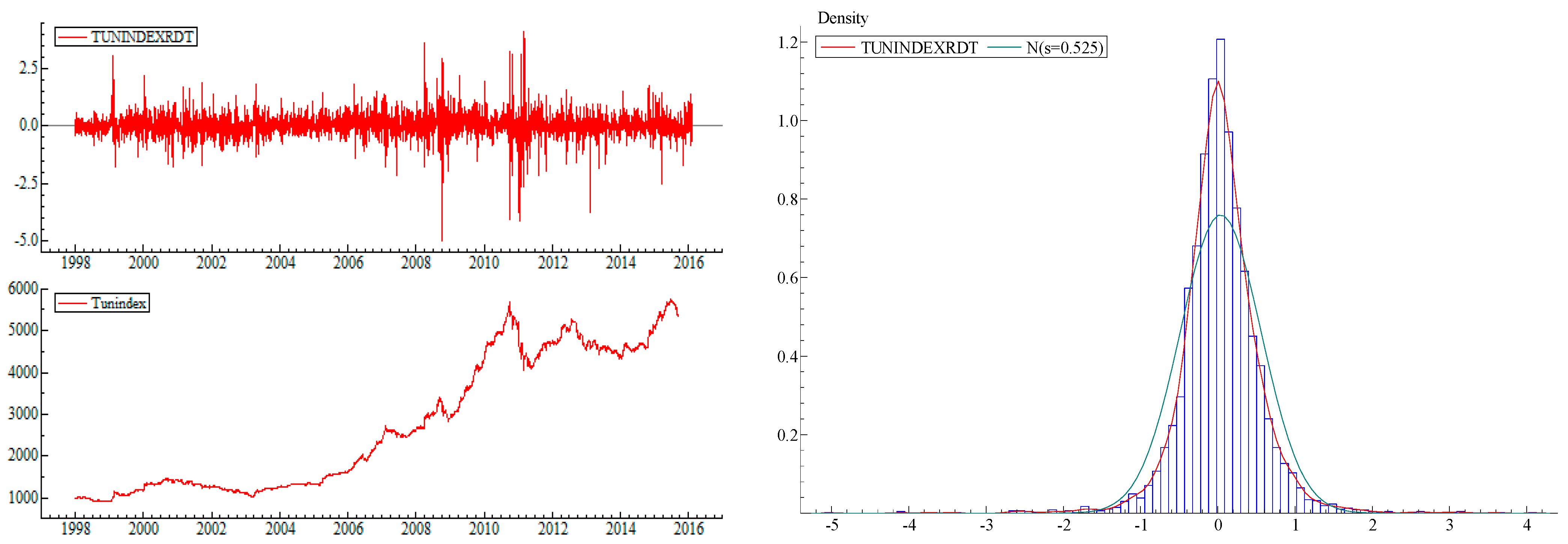
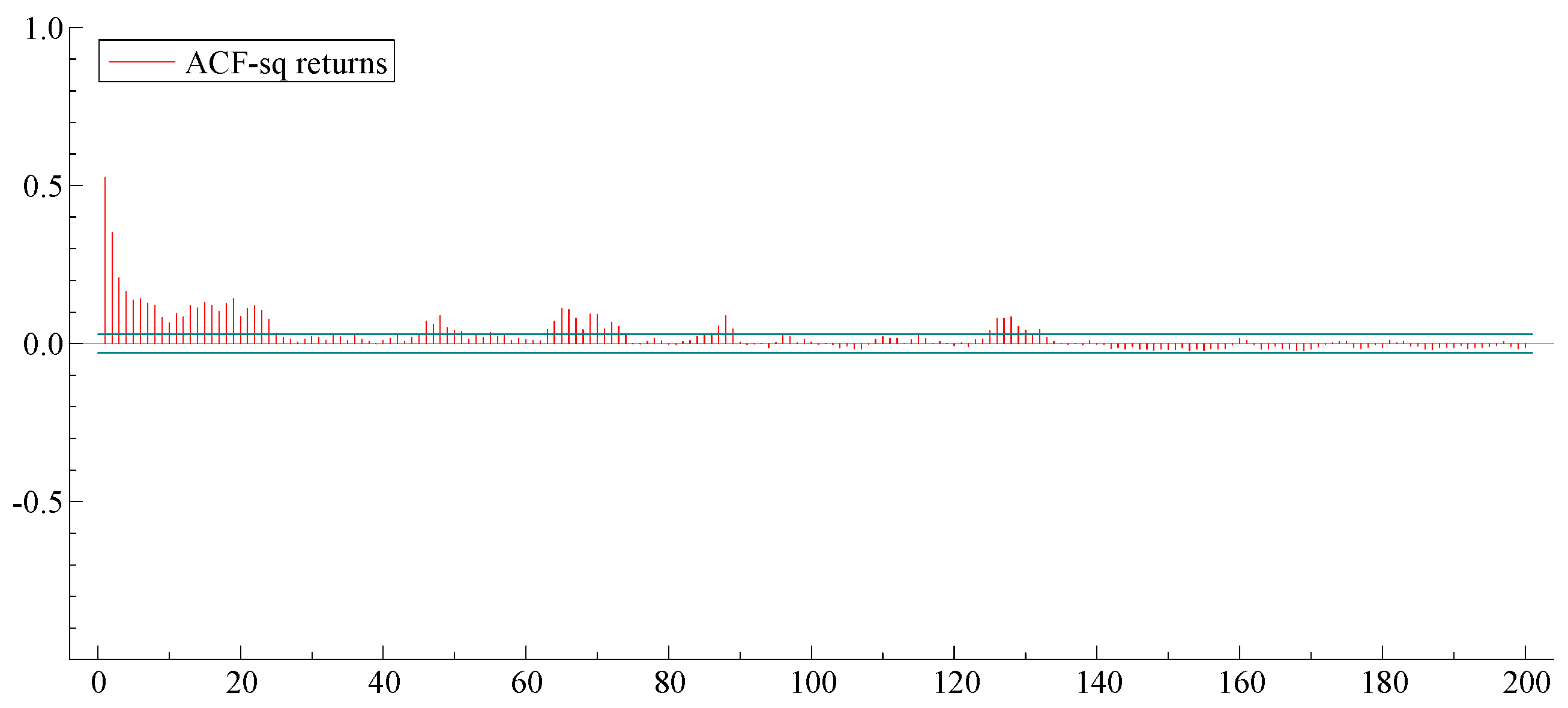
4. Data and Preliminary Statistics

We consider the daily closing prices of the Tunisia Stock Market (TUNINDEX). The latter is the major stock market index. It is a free-float capitalization-weighted index that tracks the performance of all companies listed on the Tunis Stock Exchange. Data were compiled from http://www.bvmt.com.tn/ (accessed on 9 January 2025). The total study sample spans 2 January 1998 to 6 October 2020. This period was subdivided into two sub-periods. The in-sample period ranges from 2 January 1998 to 16 September 2015 (4405 observations). The remaining 1260 observations (5 × 252) were retained for the out-of-sample forecasts. These sample data cover the Tunisian revolution events and the recent oil crashes. Figure 1 plots the evolution of daily prices. The graphical evidence shows that the series fluctuates randomly around zero and displays clustering volatility, meaning that large (or small) index price changes tend to be followed by other large (or small) index price changes of either sign (negative or positive) and are time-dependent. The continuously compounded returns are defined as $r_t=100\ast \left[\log \left(p_t\right)-\log \left(p_{t-1}\right)\right]$, where $p_t$ is the price on day $t$.

Table 1. Statistical properties of the TUNINDEX returns.

Panel A: Basic descriptive statistics
Mean	0.038027
Median	0.021586
Maximum	4.1086
Minimum	−5.0037
Std. dev	0.52516
Skewness	−0.285003
Kurtosis	13.98541
JB	22,209.31 ***
Q(10)	503.68 ***
Q2(10)	2439.0 ***
${\mathrm{Q}}_{\left|{\mathrm{r}}_{\mathrm{t}}\right|}\left(1000\right)$	6450.8 ***
Panel B: Unit root tests
ADF	−27.45200 ***
PP	−48.60005 ***
Panel C: Heteroskedasticity test
ARCH LM test	175.3621 ***

Note: *** denotes statistical significance at the 1% level. Q(10) and Q²(10) are Box–Pierce statistics applied to returns and the square of returns, respectively. Mackinnon’s 1% critical value is −3.9657 for the augmented Dickey–Fuller and Phillips–Perron (PP).

reports the results of the descriptive statistics. The mean returns of TUNINDEX are positive, indicating that positive changes in the index outnumber negative ones. The skewness value was negative, indicating asymmetry. The kurtosis values show evidence of leptokurtic tails. The result of the Jarque–Bera test rejected the null hypothesis of a Gaussian distribution. The conventional ADF unit root and KPSS results revealed that the TUNINDEX return series is stationary. The unconditional density function of the returns visualized in Figure 1 appears symmetrical, proving that the skewness coefficient is influenced by the time dependence detected in the square of the returns of the index (Figure 2). We can thus affirm that the distribution of the series is far from normal. In addition, the preliminary results indicate that the return distribution is symmetric, which may exclude the choice of Skewed Student distribution.

Table 2. GPH, GSP and R/V test results.

Geweke and Porter-Hudak (1983) test
Squared returns
m = T0.5	0.3373 [0.0001]
m = T0.6	0.2376 [0.0000]
m = T0.8	0.2468 [0.0000]
Absolute returns
m = T0.5	0.4776 [0.0000]
m = T0.6	0.3346 [0.0000]
m = T0.8	0.3190 [0.0000]
Robinson and Henry (1999) test
Squared returns
m = T/4	0.2491 [0.0000]
m = T/16	0.3276 [0.0000]
m = T/64	0.3141 [0.0000]
Absolute returns
m = T0.5	0.5415 [0.0000]
m = T0.6	0.3935 [0.0000]
m = T0.8	0.3425 [0.0000]
Lo (1991) test
Squared returns
m = 10	2.3516
m = 40	1.7475
m = 110	1.4550
Absolute returns
m = 10	2.5661
m = 40	1.8627
m = 110	1.5167

Notes: (r_t), (r²_t), and |r_t| are the log return, squared log return, and absolute log return, respectively. m denotes the bandwidth for Geweke and Porter-Hudak’s (1983) and Gaussian semiparametric (GSP) Robinson and Henry (1999) tests, respectively.

reports on the LM test results. These findings show that the volatility of the Tunisian stock market persist overtime. LM GARCH- class models are then suggested as a tool for describing the volatility behaviour of the TUNINDEX returns. This result is consistent with the autocorrelation function of squared returns (Figure 2) which indicates that returns are higher as well as remain significantly positive throughout numerous lags. Specifically, it exhibits a gradual decline with a hyperbolic rate, demonstrating the time series’ strong autocorrelation up to a lengthy lag.

5. Empirical Results

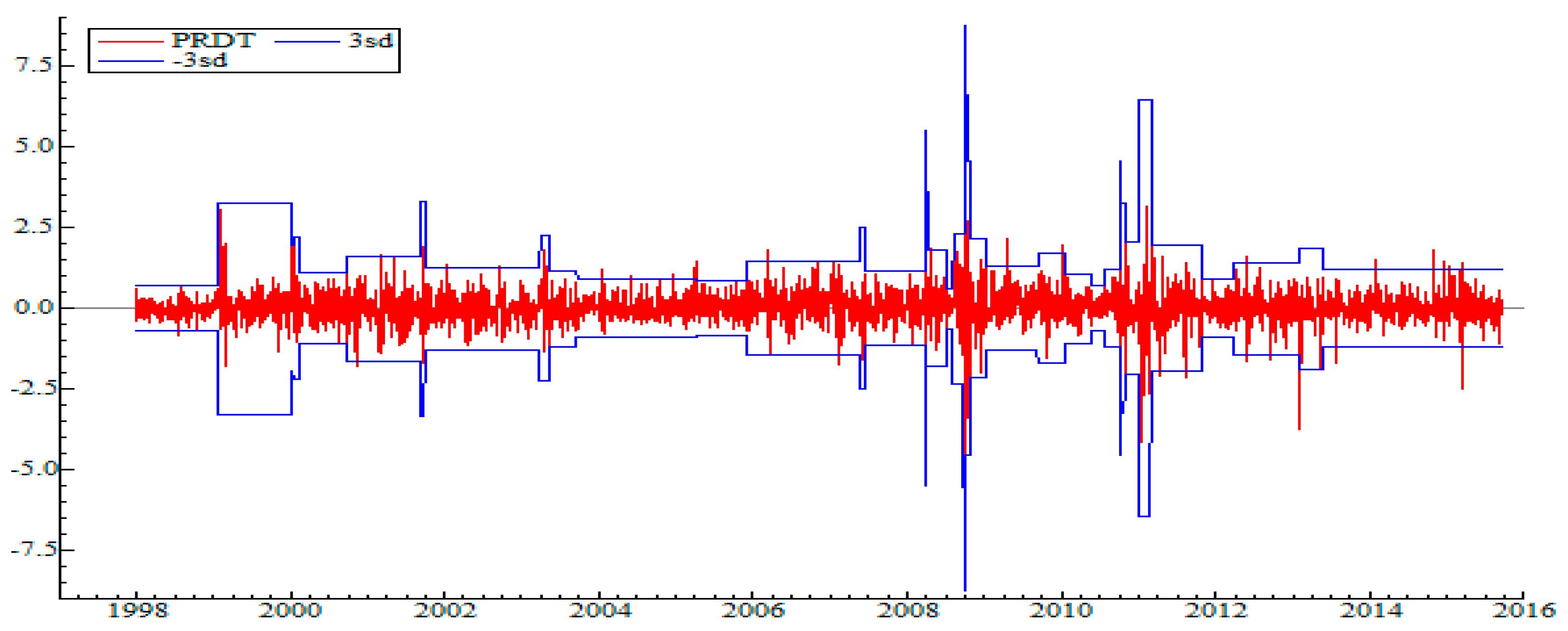
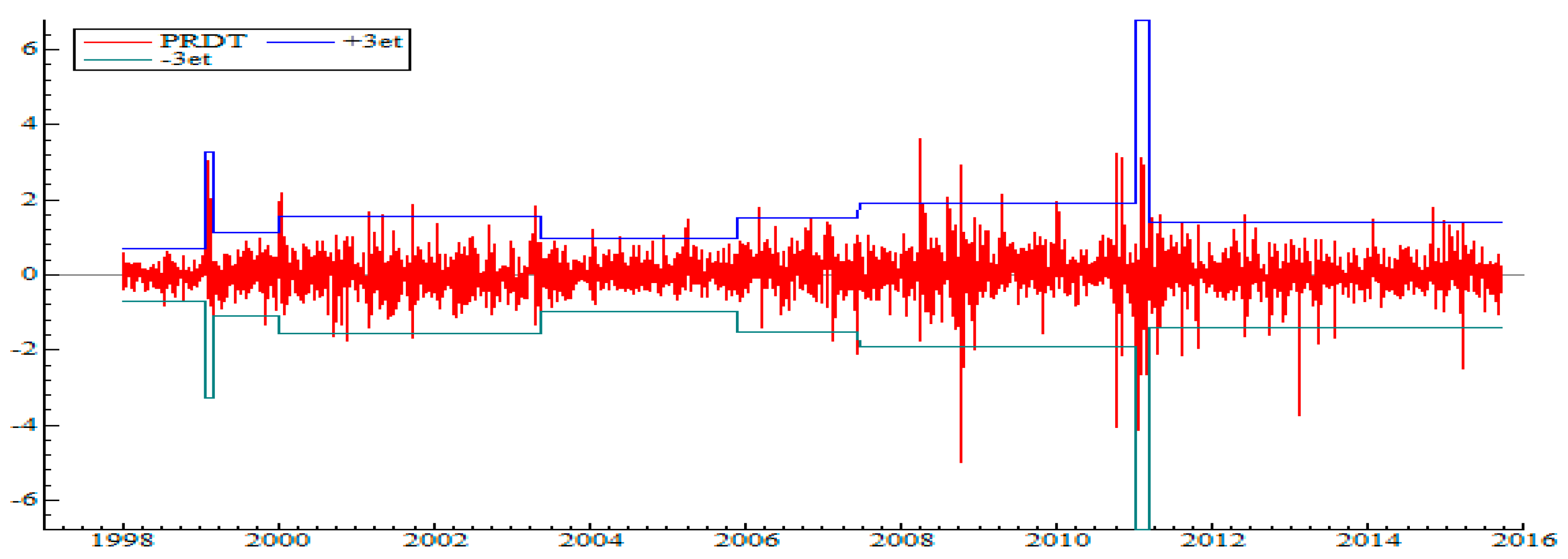
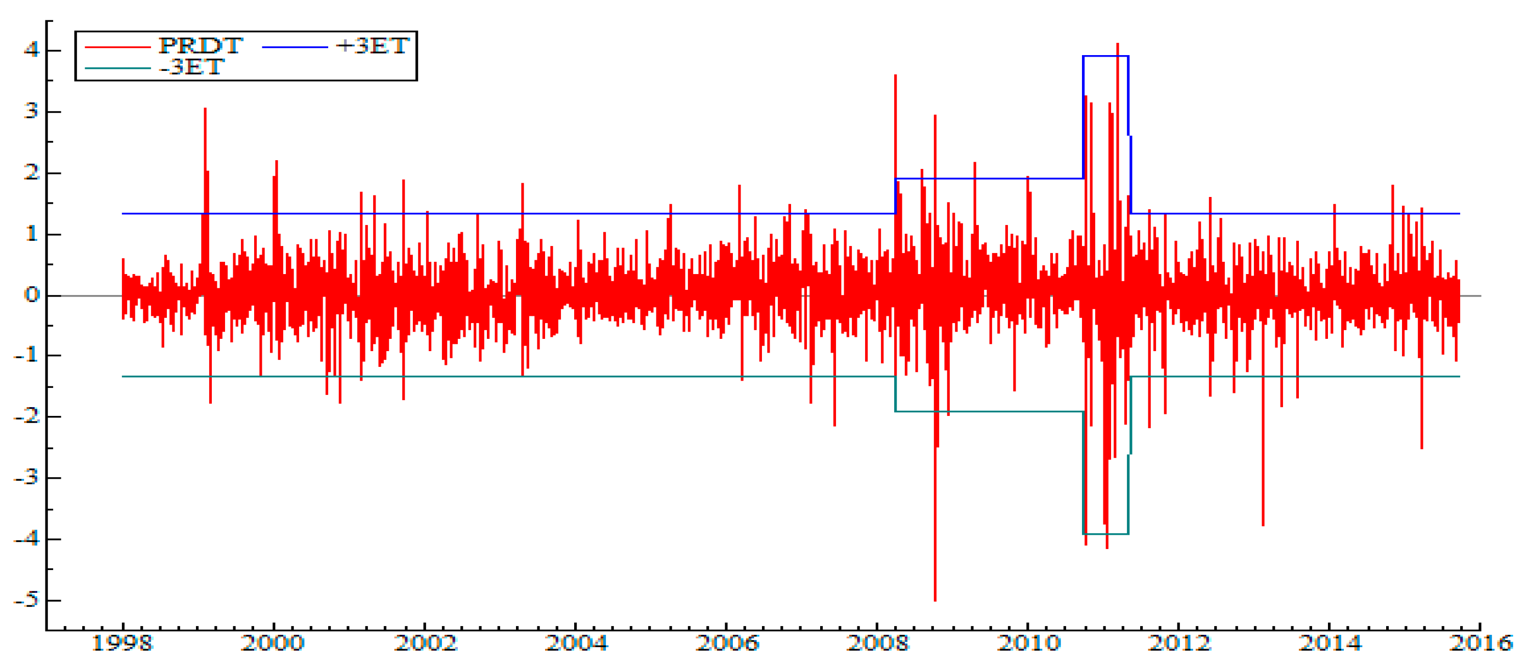
5.1. Detection of Regime Change Points in the Variance

In accordance with Souffargi and Boubaker (2022), we apply Inclan and Tiao’s (1994) ICSS algorithm and the modified ICSS developed by Sansó et al. (2004). The variance regimes determined using the ICSS algorithm are presented in

Table 3. Structural breakpoints in volatility as detected by the ICSS and modified ICSS algorithm.

T	κ1	κ2
27-01-1999 02-03-1999 05-01-2000 14-01-2000 10-02-2000 21-09-2000 14-09-2001 01-10-2001 31-03-2003 16-05-2003 22-09-2003 31-03-2005 08-04-2005 30-11-2005 24-05-2007 18-06-2007 27-03-2008 04-04-2008 11-07-2008 07-08-2008 29-09-2008 08-10-2008 23-10-2008 12-01-2009 11-09-2009 18-01-2010 24-05-2010 26-07-2010 05-10-2010 07-10-2010 02-11-2010 07-01-2011 08-03-2011 26-10-2011 30-03-2012 05-02-2013 28-05-2013	27-01-1999 02-03-1999 05-01-2000 22-05-2003 30-11-2005 18-06-2007 07-01-2011 08-03-2011	27-03-2008 01-10-2010 09-05-2011

Notes: This table reports the results of Inclan and Tiao (1994) and Sansó et al. (2004) for structural breaks in the Tunisian market’s daily returns.

. The number of breakpoints was 38 for ICSS (IT), 7 for ICSS (${\kappa }_1$), and 3 for ICSS (${\kappa }_2$). The dates are not the same for the three statistics, but there is a coincidence in the very-high-volatility regime (Figure 3, Figure 4 and Figure 5):

• In 2008, a high-volatility regime was linked to the 2008 global economic and financial crisis.
• Late 2010–early 2011: The most turbulent and volatile regime, corresponding to popular uprisings, that is, the Tunisian revolution.
• May 2011: Return to relative calm directly linked to post-revolutionary hope (elections, democracy, and optimism).

These patterns indicate that the stock market is sensitive to national and global news. Regime changes indicate structural breaks in the unconditional variance process. In the following, structural breakpoints are incorporated into the conditional variance equation of GARCH-type models in the form of dummy variables.

5.2. DML GARCH-Type Models with Structural Break Estimation Results and Diagnostics

The estimated results3 indicate that models with dummy variables for sudden changes in variance are more relevant and confirm that the distribution of the series is far from the normal distribution. One of the most interesting findings of this study was that heavy-tailed distributions performed better when dummy variables were considered. In addition, the domination of Student’s t distribution cannot be called into question for models with and without dummy variables. Moreover, the comparison of the synthetic statistics shows that the HYGARCH model is more relevant for describing the conditional variance since all the synthetic statistics carried out on the residuals are strongly reduced. Thus, the ICSS (IT)-HYGARCH model appears to be the most satisfactory representation for describing the volatility of the TUNINDEX index in the sample. The estimation results for the ARFIMA-HYGARCH–Student model with dummies are presented in

Table 4. ICSS (IT)-ARFIMA (1, d, 2)-HYGARCH under Student-t innovation’s distribution.

	Coefficient	t-Prob
d-ARFIMA	0.0888 ***	0.0000
AR(1)	−0.6624 ***	0.0000
MA(1)	0.8058 ***	0.0000
MA(2)	0.1318 ***	0.0000
IT1	0.9834 ***	0.0936
IT2	−0.5366 *	0.0222
IT3	1.0875 *	0.0667
IT4	−0.6598	0.1883
IT5	−0.1418	0.1184
IT6	0.2431	0.1756
IT7	0.6586 *	0.0938
IT8	−0.4959 *	0.0627
IT9	0.3859 **	0.0343
IT10	−0.1417	0.1131
IT11	−0.0548 *	0.0581
IT12	0.7669 ***	0.0070
IT13	−0.6376 ***	0.0059
IT14	0.1770 **	0.0413
IT15	0.5358 *	0.0908
IT16	−0.3076 *	0.0767
IT17	3.7894 *	0.0800
IT18	−2.9453 *	0.0935
IT19	−0.1639 ***	0.0000
IT20	0.6961 **	0.0438
IT21	10.0941	0.1166
IT22	−9.6629 *	0.0885
IT23	0.3536	0.6961
IT24	−0.1232	0.3146
IT25	0.1994	0.1625
IT26	−0.0701	0.2162
IT27	−0.0783 ***	0.0000
IT28	0.0693	0.2036
IT29	9.2775	0.2174
IT30	−8.9530	0.1988
IT31	1.6249 *	0.0819
IT32	−1.6244 **	0.0447
IT33	4.3378 ***	0.0098
IT34	−2.1860 ***	0.0017
IT35	−0.3154 ***	0.0000
IT36	0.0615	0.5207
IT37	0.0942	0.7317
IT38	−0.1411 ***	0.0000
d-Figarch	0.2268 ***	0.0000
ARCH (Phi1)	0.9537 ***	0.0000
GARCH (Beta1)	0.9623 ***	0.0000
Student (DF)	8.4889 ***	0.0000
Log Alpha (HY)	0.1202 *	0.0597
Q2 (20)	18.3968	0.4298
ARCH (10)	0.6815	0.7426

Notes: *, ** and *** denote significance at the 10%; 5%; and 1% level, respectively.

. Of the 38 dummy variables incorporated in the conditional volatility equation, the dummies IT32, IT33, IT34, IT35, and IT38 constitute the points of structural change during the revolutionary and post-revolutionary periods. These variables are highly significant at the 5% level. More interestingly, our results reveal that the weak form of the Tunisian stock market is inefficient. In fact, the regulatory framework related to information efficiency is still relatively weak in terms of the transparency and disclosure of information.

5.3. Model Predictive Performance

Table 5. Comparison of the predictive performance of the ARFIMA-FIGARCH-St, ARFIMA-FIAPARCH-St and ARFIMA-HYGARCH-St models without and with dummies.

h = 1	ARFIMA-FIGARCH-St		ARFIMA-ICSS-FIGARCH-St		ARFIMA-κ1-FIGARCH-St		ARFIMA-κ2-FIGARCH-St
MSE	0.009254	(0.004818)	0.003512	(0.002793)	0.004068	(0.004236)	0.003893	(0.004425)
MAE	0.0962	(0.06941)	0.05926	(0.05284)	0.06378	(0.06508)	0.06239	(0.06652)
TIC	0.4274	(0.4679)	0.2262	(0.401)	0.2477	(0.4519)	0.241	(0.4573)
RMSE	0.0962	(0.06941)	0.05926	(0.05284)	0.06378	(0.06508)	0.06239	(0.06652)
h = 5	ARFIMA FIAPARCH-St		ARFIMA-ICSS-FIAPARCH-St		ARFIMA-κ1-FIAPARCH-St		ARFIMA-κ2-FIAPARCH-St
MSE	0.003966	(0.004414)	0.003349	(0.003923)	0.009386	(0.004606)	0.003933	(0.00437)
MAE	0.06298	(0.06644)	0.05787	(0.06264)	0.09688	(0.06786)	0.06272	(0.0661)
TIC	0.2438	(0.457)	0.2197	(0.4424)	0.4317	(0.4623)	0.2426	(0.4558)
RMSE	0.06298	(0.06644)	0.05787	(0.06264)	0.09688	(0.06786)	0.06272	(0.0661)
h = 10	ARFIMA-HYGARCH-St		ARFIMA-ICSS-HYGARCH-St		ARFIMA-κ1-HYGARCH-St		ARFIMA-κ2-HYGARCH-St
MSE	0.003941	(0.004691)	0.00955	(0.005005)	0.009379	(0.005505)	0.003856	(0.004558)
MAE	0.06278	(0.06849)	0.09772	(0.07074)	0.09684	(0.07419)	0.06209	(0.06751)
TIC	0.2429	(0.4646)	0.4371	(0.4726)	0.4315	(0.4845)	0.2396	(0.461)
RMSE	0.06278	(0.06849)	0.09772	(0.07074)	0.09684	(0.07419)	0.06209	(0.06751)

Notes: This table reports 1-, 5-, and 10-step-ahead forecasts of the conditional mean (on the left) and conditional variance (on the right). MSE is Mean Squared Error, MAE is the mean absolute prediction error, TIC is the Theil Inequality Coefficient, and RMSE is Root Mean Squared Error.

lists the forecast evaluation criteria (MSE, MAE, TIC, RMSE) calculated for the models. The forecast results show that the models without dummies are beaten by all models tested for all forecast horizons4.

The FIAPARCH model appears to outperform the HYGARCH model in terms of forecasting, as forecast errors are the smallest, regardless of the forecast criterion and period. This result is valid in terms of the conditional mean and variance. Thus, the persistence of volatility modelled using the FIAPARCH model, combined with the introduction of structural breakpoints, significantly improves volatility forecasting.

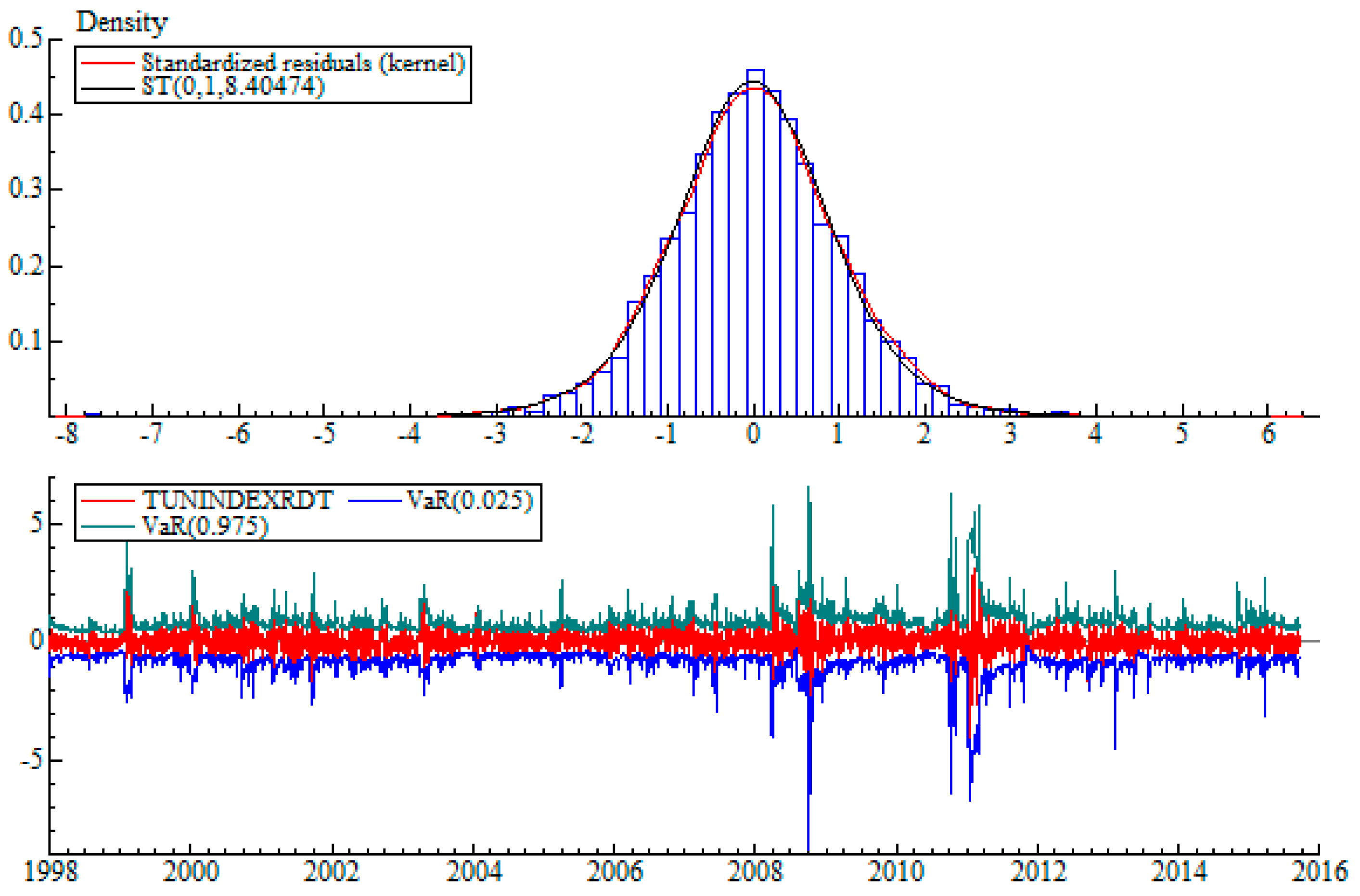
5.4. Value-at-Risk and ES Modelling

Backtesting is essential to validate any model. Backtesting consists of comparing the calculated VaR with the actual realized profits and losses. Thus, for a 99% confidence level, the actual losses should exceed the VaR forecasts in only 1% of cases. Otherwise, we are forced to question the validity of the model.

5.4.1. Backtesting In-Sample

To test the contribution of the double long memory model with structural breaks to VaR calculations, we compare their predictive power with a “classic” VaR method: the RiskMetrics method. The principle of the latter is to assign more weight to recent data than to old data, which makes estimators more responsive to changes in market conditions. This reactivity is essential, as markets are composed of a succession of calm and turbulent periods. While the transition from one period to another remains statistically unpredictable, it is important for estimators to be able to detect and translate a change in period as quickly as possible, hence the interest in this method. Formally, the RiskMetrics model is equivalent to the IGARCH (1,1) model with λ = 0.94 for daily data.

The analysis of

Table 6. In-sample backtesting of VaR and ES for short and long positions.

	Panel A. Short Position				Panel B. Long Position
Quantile	Success Rate	Kupiec LRT	DQT	ESF	Quantile	Failure Rate	Kupiec LRT	DQT	ESF
Without dummies ARFIMA-FIGARCH
0.95000	0.93666	15.267 (9.3335 × 10−5)	19.780 (0.0030303)	0.92612	0.050000	0.051078	0.10711 (0.74346)	4.2166 (0.64739)	−0.94183
0.97500	0.97072	3.1477 (0.076033)	8.9401 (0.17698)	1.0682	0.025000	0.028150	1.7239 (0.18919)	12.806 (0.046224)	−1.0756
0.99000	0.98842	1.0541 (0.30456)	6.2504 (0.39574)	1.2728	0.010000	0.010443	0.085948 (0.76939)	7.4811 (0.27863)	−1.4611
0.99500	0.99410	0.68136 (0.40912)	12.554 (0.050692)	1.4565	0.0050000	0.0063564	1.4996 (0.22073)	12.377 (0.054065)	−1.7704
0.99750	0.99614	2.7954 (0.094537)	45.438 (3.8305 × 10−8)	1.4680	0.0025000	0.0038593	2.7954 (0.094537)	3.7817 (0.70619)	−1.8591
ARFIMA-FIAPARCH
0.95000	0.94302	4.3327 (0.037386)	10.779 (0.095454)	0.93101	0.050000	0.048354	0.25387 (0.61437)	3.1743 (0.78667)	−0.95550
0.97500	0.97276	0.88288 (0.34741)	7.0652 (0.31486)	1.0806	0.025000	0.024064	0.16044 (0.68875)	5.4236 (0.49073)	−1.1233
0.99000	0.98956	0.085948 (0.76939)	2.9911 (0.80997)	1.2187	0.010000	0.0095346	0.097882 (0.75439)	3.0611 (0.80113)	−1.5197
0.99500	0.99432	0.38690 (0.53393)	12.949 (0.043849)	1.4907	0.0050000	0.0056754	0.38690 (0.53393)	7.0252 (0.31852)	−1.7746
0.99750	0.99659	1.2992 (0.25436)	1.8026 (0.93693)	1.4840	0.0025000	0.0024972	1.4229 × 10−5 (0.99699)	0.13948 (0.99995)	−2.1762
ARFIMA-HYGARCH
0.95000	0.94597	1.4689 (0.22552)	5.8227 (0.44334)	0.94781	0.050000	0.044949	2.4456 (0.11786)	5.7780 (0.44851)	−0.98197
0.97500	0.97594	0.16044 (0.68875)	2.8905 (0.82247)	1.1007	0.025000	0.021793	1.9410 (0.16356)	5.8868 (0.43598)	−1.1677
0.99000	0.99047	0.097882 (0.75439)	3.0021 (0.80859)	1.2725	0.010000	0.0086266	0.88021 (0.34814)	4.2017 (0.64940)	−1.5851
0.99500	0.99501	2.8530 × 10−5 (0.99574)	15.067 (0.019740)	1.3361	0.0050000	0.0047673	0.048699 (0.82534)	8.2654 (0.21929)	−1.9254
0.99750	0.99728	0.086238 (0.76902)	0.27002 (0.99963)	1.5995	0.0025000	0.0022701	0.096315 (0.75630)	0.19800 (0.99985)	−2.2720
RiskMetrics
0.95000	0.93961	9.4080 (0.0021604)	83.850 (5.5511 × 10−16)	0.97461	0.050000	0.044268	3.1642 (0.075269)	35.633 (3.2485 × 10−6)	−0.99722
0.97500	0.96549	14.628 (0.00013095)	145.48 (0.00000)	1.1196	0.025000	0.025199	0.0071123 (0.93279)	37.312 (1.5305 × 10−6)	−1.2032
0.99000	0.98138	26.340 (2.8633 × 10−7)	109.96 (0.00000)	1.3415	0.010000	0.014302	7.2664 (0.0070255)	57.188 (1.6735 × 10−10)	−1.4571
0.99500	0.98729	36.829 (1.2893 × 10−9)	237.16 (0.00000)	1.4927	0.0050000	0.0088536	10.684 (0.0010808)	44.471 (5.9610 × 10−8)	−1.6461
0.99750	0.98888	70.648 (0.00000)	274.46 (0.00000)	1.5367	0.0025000	0.0065834	20.258 (6.7667 × 10−6)	90.773 (0.00000)	−1.8042
With dummies ARFIMA-FIGARCH
0.95000	0.94279	4.6131 (0.031729)	18.449 (0.0052031)	0.89055	0.050000	0.048808	0.13273 (0.71562)	4.5418 (0.60377)	−0.85211
0.97500	0.97299	0.71512 (0.39775)	4.7810 (0.57219)	1.0030	0.025000	0.025426	0.032563 (0.85680)	5.9818 (0.42523)	−0.99780
0.99000	0.98978	0.020549 (0.88601)	2.6673 (0.84929)	1.1595	0.010000	0.011124	0.54213 (0.46155)	3.4825 (0.74630)	−1.2357
0.99500	0.99432	0.38690 (0.53393)	1.2378 (0.97498)	1.1623	0.0050000	0.0061294	1.0532 (0.30477)	2.1823 (0.90219)	−1.3679
0.99750	0.99682	0.74777 (0.38718)	1.1009 (0.98150)	1.4176	0.0025000	0.0027242	0.086238 (0.76902)	0.27002 (0.99963)	−1.5662
ARFIMA-FIAPARCH
0.95000	0.94597	1.4689 (0.22552)	13.086 (0.041685)	0.90051	0.050000	0.046538	1.1367 (0.28636)	3.6434 (0.72481)	−0.87643
0.97500	0.97526	0.011827 (0.91340)	5.3098 (0.50474)	1.0315	0.025000	0.023610	0.35589 (0.55080)	4.8888 (0.55815)	−1.0177
0.99000	0.99024	0.025482 (0.87317)	2.7578 (0.83857)	1.1836	0.010000	0.010216	0.020549 (0.88601)	2.5986 (0.85727)	−1.2499
0.99500	0.99523	0.048699 (0.82534)	0.54004 (0.99732)	1.2352	0.0050000	0.0047673	0.048699 (0.82534)	0.54004 (0.99732)	−1.5277
0.99750	0.99728	0.086238 (0.76902)	0.27002 (0.99963)	1.4970	0.0025000	0.0024972	1.4229 × 10−5 (0.99699)	0.13948 (0.99995)	−1.5826
ARFIMA-HYGARCH
0.95000	0.94665	1.0185 (0.31287)	9.4534 (0.14964)	0.91518	0.050000	0.043587	3.9794 (0.046060)	6.6709 (0.35236)	−0.89863
0.97500	0.97616	0.24841 (0.61820)	3.1524 (0.78949)	1.0865	0.025000	0.022247	1.4211 (0.23323)	8.5323 (0.20164)	−1.0450
0.99000	0.99115	0.60828 (0.43544)	2.9439 (0.81586)	1.2327	0.010000	0.0083995	1.2052 (0.27228)	3.5046 (0.74335)	−1.3337
0.99500	0.99591	0.78866 (0.37450)	1.0481 (0.98372)	1.3101	0.0050000	0.0045403	0.19310 (0.66035)	0.61174 (0.99620)	−1.5572
0.99750	0.99750	1.4229 × 10−5 (0.99699)	0.13948 (0.99995)	1.5695	0.0025000	0.0018161	0.91363 (0.33915)	0.87963 (0.98977)	−1.8439

shows that the results of the backtesting in-sample indicate poor performance of the RiskMetrics model. This model proved to be inappropriate for both the long and short positions. The inclusion of structural breakpoints in the conditional variance equation significantly improves the power of all three models to provide a more relevant VaR estimate. Interestingly, when structural breakpoints are considered, p-values increase when a very high level of confidence is required. This leads us to highlight an important result: the introduction of structural breakpoints in the variance significantly improves the prediction of extreme tails.

For long positions, ARFIMA-FIGARCH with structural breaks and ARFIMA–FIAPARCH with structural breaks are ahead of ARFIMA-HYGARCH with structural breaks. In addition, as depicted in Figure 6, ARFIMA-FIAPARCH with structural breaks proves its slight predominance for long positions. For short positions, the ARFIMA-HYGARCH model with structural breaks performed better. The p-values were all greater than 0.05.

5.4.2. Backtesting Out-of-Sample

The results of the out-of-sample backtesting of the selected models, carried out for a rolling fifty-day window, are presented in

Table 7. Out-of-sample backtesting of VaR and ES for short and long positions, 2015–2020.

	Panel A. Short Position				Panel B. Long Position
Quantile	Success Rate	Kupiec LRT	DQT	ESF	Quantile	Failure Rate	Kupiec LRT	DQT	ESF
With dummies ARFIMA-HYGARCH
0.95000	0.94762	0.14817 (0.70029)	0.15038 (0.69818)	0.34162	0.050000	0.049206	0.016793 (0.89689)	0.016708 (0.89715)	−0.42699
0.97500	0.97381	0.072153 (0.78823)	0.073260(0.78665)	0.38899	0.025000	0.025397	0.0080984 (0.92829)	0.0081400 (0.92811)	−0.49772
0.99000	0.99127	0.21442 (0.64333)	0.20523 (0.65053)	0.46804	0.010000	0.0063492	1.9489 (0.16271)	1.6963 (0.19277)	−0.56897
0.99500	0.99603	0.29023 (0.59007)	0.26960 (0.60360)	0.56656	0.0050000	0.0031746	0.97017 (0.32464)	0.84390 (0.35828)	−0.65495
0.99750	0.99841	0.48403 (0.48660)	0.42089 (0.51649)	0.38525	0.0025000	0.0023810	0.0072769 (0.93202)	0.0071608 (0.93256)	−0.77941
ARFIMA-FIAPARCH
0.95000	0.91587	25.868 (3.6557 × 10−7)	30.894 (2.7253 × 10−8)	0.32255	0.050000	0.071429	10.815 (0.0010067)	12.180 (0.00048293	−0.38649
0.97500	0.95714	13.626 (0.00022305)	16.484 (4.9075 × 10−5)	0.38541	0.025000	0.040476	10.459 (0.0012208)	12.381 (0.00043374)	−0.46576
0.99000	0.98175	6.9696 (0.0082905)	8.6708 (0.0032334)	0.43339	0.010000	0.016667	4.7114 (0.029964)	5.6566 (0.017390)	−0.69602
0.99500	0.98968	5.4703 (0.019343)	7.1612 (0.0074497)	0.46698	0.0050000	0.0071429	1.0260 (0.31111)	1.1630 (0.28085)	−0.68582
0.99750	0.99524	2.0388 (0.15334)	2.5850 (0.10788)	0.55245	0.0025000	0.0039683	0.92308 (0.33667)	1.0892 (0.29664)	−0.74953
ARFIMA-FIGARCH
0.95000	0.92619	13.199 (0.00028015)	15.038 (0.00010539)	0.32951	0.050000	0.062698	3.9723 (0.046255)	4.2774 (0.038623)	−0.40151
0.97500	0.96270	6.8114 (0.0090576)	7.8225 (0.0051598)	0.37591	0.025000	0.034921	4.5374 (0.033162)	7.8225 (0.0051598)	−0.48474
0.99000	0.98651	1.3991 (0.23687)	1.5520 (0.21284)	0.43983	0.010000	0.0095238	0.029325 (0.86403)	0.028860 (0.86510)	−0.58175
0.99500	0.99206	1.8516 (0.17359)	2.1839 (0.13946)	0.47945	0.0050000	0.0055556	0.075438 (0.78358)	0.078169 (0.77979)	−0.62533
0.99750	0.99603	0.92308 (0.33667)	1.0892 (0.29664)	0.56656	0.0025000	0.0023810	0.0072769 (0.93202)	0.0071608 (0.93256)	−0.77941
Without dummies ARFIMA-HYGARCH
0.95000	0.94444	0.79149 (0.37365)	0.81871 (0.36556)	0.34067	0.050000	0.049206	0.016793 (0.89689)	0.016708 (0.89715)	−0.43280
0.97500	0.97302	0.1984 (0.65597)	0.20350 (0.65191)	0.39069	0.025000	0.026190	0.072153 (0.78823)	0.073260 (0.78665)	−0.46395
0.99000	0.99127	0.21442 (0.64333)	0.20523 (0.65053)	0.46804	0.010000	0.0063492	1.9489 (0.16271)	1.6963 (0.19277)	−0.56897
0.99500	0.99603	0.29023 (0.59007)	0.26960 (0.60360)	0.56656	0.0050000	0.0031746	0.97017 (0.32464)	0.84390 (0.35828)	−0.65495
0.99750	0.99841	0.48403 (0.48660)	0.42089 (0.51649)	0.38525	0.0025000	0.0023810	0.0072769 (0.93202)	0.0071608 (0.93256)	−0.77941
ARFIMA-FIAPARCH
0.95000	0.92063	19.563 (9.7349 × 10−6)	22.874 (1.7299 × 10−6)	0.32870	0.050000	0.073810	13.199 (0.00028015)	15.038 (0.00010539)	−0.37557
0.97500	0.95794	12.531 (0.00040031)	15.051 (0.00010465)	0.38982	0.025000	0.038889	8.5501 (0.0034551)	9.9715 (0.0015898)	−0.47546
0.99000	0.98175	6.9696 (0.0082905)	8.6708 (0.0032334)	0.44786	0.010000	0.015873	3.7254 (0.053591)	4.3899 (0.036152)	−0.70995
0.99500	0.99048	4.0905 (0.043124)	5.1831 (0.022808)	0.47913	0.0050000	0.0087302	2.8792 (0.089728)	3.5240 (0.060487)	−0.78024
0.99750	0.99524	2.0388 (0.15334)	2.5850 (0.10788)	0.55245	0.0025000	0.0039683	0.92308 (0.33667)	1.0892 (0.29664)	−0.74953
ARFIMA-FIGARCH
0.95000	0.92619	13.199 (0.00028015)	15.038 (0.00010539)	0.33053	0.050000	0.065873	6.1032 (0.013494)	6.6834 (0.0097316)	−0.38926
0.97500	0.96587	3.8723 (0.049090)	4.3061 (0.037977)	0.36784	0.025000	0.035714	5.2496 (0.021951)	5.9341 (0.014851)	−0.48170
0.99000	0.98413	3.7254 (0.053591)	4.3899 (0.036152)	0.44005	0.010000	0.011111	0.15167 (0.69695)	0.15713 (0.69182)	−0.68124
0.99500	0.99206	1.8516 (0.17359)	2.1839 (0.13946)	0.47945	0.0050000	0.0055556	0.075438 (0.78358)	0.078169 (0.77979)	−0.62533
0.99750	0.99603	0.92308 (0.33667)	1.0892 (0.29664)	0.56656	0.0025000	0.0023810	0.0072769 (0.93202)	0.0071608 (0.93256)	−0.77941
RiskMetrics
0.95000	0.93492	5.5311 (0.018682)	6.0317 (0.014051)	0.80584	0.050000	0.051587	0.066174 (0.79699)	0.066834 (0.79600)	−1.0352
0.97500	0.95952	10.459 (0.0012208)	12.381 (0.00043374)	0.93511	0.025000	0.033333	3.2553 (0.071193)	3.5897 (0.058137)	−1.1936
0.99000	0.97778	14.107 (0.00017267)	19.012 (1.2988 × 10−5)	1.0623	0.010000	0.020635	11.013 (0.00090463)	14.395 (0.00014822)	−1.4150
0.99500	0.98492	16.677 (4.4318 × 10−5)	25.730 (3.9263 × 10−7)	1.1197	0.0050000	0.014286	14.503 (0.00013993)	21.838 (2.9670 × 10−6)	−1.6806
0.99750	0.98810	23.232 (1.4362 × 10−6)	44.690 (2.3080 × 10−11)	1.2002	0.0025000	0.011111	20.160 (7.1217 × 10−6)	37.466 (9.3026 × 10−10)	−1.8526

. The results confirmed the poor performance of the RiskMetrics model, despite its popularity and reputation in the field of VaR estimation. This is consistent with the findings of Giot and Laurent (2004) and So and Philip (2006). The invalidity of the RiskMetrics approach lies in the fact that the VaR measure assumes a normal distribution. This assumption contradicts reality. This law is clearly not adapted to the Tunisian context because it considerably underestimates extreme events, which are the most important events in the VaR calculations. The results also suggest the superiority of the ARFIMA-HYGARCH model with breaks. Thus, all of these analyses allow us to emphasize the following:

The dual long-memory models outperformed the RiskMetrics method at all the confidence levels. The empirical distribution of the TUNINDEX stock market returns is characterized by fat tails containing many extreme values whose probabilities of occurrence are higher than those assumed by the normal distribution. This justifies the choice of a conditional innovation density function other than the normal distribution, that is, a Student distribution. Our findings are in line with Aloui and Ben Hamida (2014).

The out-of-sample forecasting of VaR using the ARFIMA-HYGARCH model seems more relevant. Indeed, the p-value of the LR test is usually high, and the null hypothesis of model validity is often accepted. The innovative aspect of the dual long-memory model with structural breaks has succeeded in accounting for both long-term dependence on the mean and volatility of TUNINDEX returns, thereby delivering an accurate VaR and ES estimators. Indeed, these processes have the advantage of taking into account both short-term behaviour via autoregressive and moving-average terms and long-term behaviour via the fractional integration parameter. In particular, the inclusion of structural breakpoints in the conditional variance equation significantly improved the prediction of extreme events.

Market efficiency is closely linked to the absence of memory. The efficiency hypothesis was associated with the random walk model. Tunisian stock prices are far from random walks, and the return processes are not white noise. These results suggest that, among other things, the financial market is inefficient. The price observed in the market does not fluctuate randomly around its fundamental value, making it possible to generate abnormal returns. Our findings have significant relevance for Tunisian investors and policymakers. In fact, precise risk estimates aid investors in the development of improved hedging strategies. As for regulators, effective financial stability monitoring is made possible through improved forecasting of extreme losses. Moreover, portfolio managers benefit from upgraded risk models because they help them allocate capital more efficiently and effectively manage downside risk.

6. Conclusions

The main idea of this study is to propose an approach that can be used to model the dynamics of Tunisian stock prices more accurately and adequately, considering the character of double long memories and structural changes in variance. We propose three time-series models that incorporate both long-term dependence in the level and volatility of returns, in which one of the major contributions is the presence of structural breaks in variance. We also used four conditional innovation density functions: normal distribution, Student distribution, GED distribution, and Skewed Student distribution.

The empirical results show that the inclusion of structural breakpoints in the conditional variance equation and DLM provides better short- and long-term predictability. We integrated the student distribution as the conditional density function of innovations. This distribution could account for the excess kurtosis observed in the data. In such a framework, the innovative aspect of the ICSS-ARFIMA-HYGARCH model with Student’s t distribution succeeded in accounting for both the long-term dependence in the level and volatility of TUNINDEX index returns, excess kurtosis, and structural changes, thereby delivering an accurate estimator of VaR and expected shortfall. This method improves risk management practices, particularly in markets that are susceptible to economic and political shocks.

References

1. Abdi, A., Souffargi, W., & Boubaker, A. (2023). Family firms’ resilience during the COVID-19 pandemic: Evidence from French firms. Corporate Ownership and Control, 20(3), 1–18. [Google Scholar] [CrossRef]
2. Aggarwal, R., Inclan, C., & Leal, R. (1999). Volatility in emerging stock markets. Journal of Financial and Quantitative Analysis, 34(01), 33–55. [Google Scholar] [CrossRef]
3. Ahamada, I., & Aïssa, M. S. B. (2005). Changements Structurels dans la Dynamique de l’lnflation aux États-Unis: Approches Non Paramétriques. Annales d’Economie et de Statistique, 157–172. [Google Scholar] [CrossRef]
4. Allen, D. E., Singh, A. K., & Powell, R. J. (2013). EVT and tail-risk modelling: Evidence from market indices and volatility series. The North American Journal of Economics and Finance, 26, 355–369. [Google Scholar] [CrossRef]
5. Aloui, C., & Ben Hamida, H. (2014). Modelling and forecasting value at risk and expected shortfall for GCC stock markets: Do long memory, structural breaks, asymmetry, and fat-tails matter? The North American Journal of Economics and Finance, 29, 349–380. [Google Scholar] [CrossRef]
6. Arouri, M. E. H., Hammoudeh, S., Lahiani, A., & Nguyen, D. K. (2012). Long memory and structural breaks in modeling the return and volatility dynamics of precious metals. The Quarterly Review of Economics and Finance, 52(2), 207–218. [Google Scholar] [CrossRef]
7. Artzner, P., Delbaen, F., Eber, J. M., & Heath, D. (1999). Coherent measures of risk. Mathematical Finance, 9(3), 203–228. [Google Scholar] [CrossRef]
8. Aydogan, K., & Booth, G. G. (1988). Are there long cycles in common stock returns? Southern Economic Journal, 55, 141–149. [Google Scholar] [CrossRef]
9. Baillie, R. T., Bollerslev, T., & Mikkelsen, H. O. (1996). Fractionally integrated generalized autoregressive conditional heteroskedasticity. Journal of Econometrics, 74(1), 3–30. [Google Scholar] [CrossRef]
10. Barkoulas, J., Labys, W. C., & Onochie, J. (1997). Fractional dynamics in international commodity prices. Journal of Futures Markets, 17(2), 161–189. [Google Scholar] [CrossRef]
11. Barkoulas, J. T., & Baum, C. F. (1996). Long-term dependence in stock returns. Economics Letters, 53(3), 253–259. [Google Scholar] [CrossRef]
12. Bellalah, M., Aloui, C., & Abaoub, E. (2005). Long-range dependence in daily volatility on Tunisian stock market. International Journal of Business, 10(3), 191–216. [Google Scholar]
13. Bisaglia, L., & Guégan, D. (1998). A comparison of techniques of estimation in long memory processes. Computational Statistics & Data Analysis, 27(1), 61–81. [Google Scholar]
14. Bollerslev, T. (1986). Generalized autoregressive conditional heteroskedasticity. Journal of Econometrics, 31(3), 307–327. [Google Scholar] [CrossRef]
15. Bollerslev, T. (1987). A conditionally heteroskedastic time series model for speculative prices and rates of return. The Review of Economics and Statistics, 69, 542–547. [Google Scholar] [CrossRef]
16. Charfeddine, L., & Ajmi, A. N. (2013). The Tunisian stock market index volatility: Long memory vs. switching regime. Emerging Markets Review, 16, 170–182. [Google Scholar] [CrossRef]
17. Cheung, Y. W. (1993). Long memory in foreign-exchange rates. Journal of Business & Economic Statistics, 11(1), 93–101. [Google Scholar]
18. Cheung, Y. W., & Lai, K. S. (1995). A search for long memory in international stock market returns. Journal of International Money and Finance, 14(4), 597–615. [Google Scholar] [CrossRef]
19. Corazza, M., Malliaris, A. G., & Nardelli, C. (1997). Searching for fractal structure in agricultural futures markets. Journal of Futures Markets, 17(4), 433–473. [Google Scholar] [CrossRef]
20. Crato, N. (1994). Some international evidence regarding the stochastic memory of stock returns. Applied Financial Economics, 4(1), 33–39. [Google Scholar] [CrossRef]
21. Davidson, J. (2004). Moment and memory properties of linear conditional heteroscedasticity models, and a new model. Journal of Business & Economic Statistics, 22, 16–29. [Google Scholar]
22. Degiannakis, S. (2004). Volatility forecasting: Evidence from a fractional integrated asymmetric power ARCH skewed-t model. Applied Financial Economics, 14(18), 1333–1342. [Google Scholar] [CrossRef]
23. Degiannakis, S., Floros, C., & Dent, P. (2013). Forecasting value-at-risk and expected shortfall using fractionally integrated models of conditional volatility: International evidence. International Review of Financial Analysis, 27, 21–33. [Google Scholar] [CrossRef]
24. Diebold, F. X. (1998). The past, present, and future of macroeconomic forecasting. Journal of Economic Perspectives, 12(2), 175–192. [Google Scholar] [CrossRef]
25. Ding, Z., Granger, C. W., & Engle, R. F. (1993). A long memory property of stock market returns and a new model. Journal of Empirical Finance, 1(1), 83–106. [Google Scholar] [CrossRef]
26. DiSario, R., Saraoglu, H., McCarthy, J., & Li, H. (2008). Long memory in the volatility of an emerging equity market: The case of Turkey. Journal of International Financial Markets, Institutions and Money, 18(4), 305–312. [Google Scholar] [CrossRef]
27. Engle, R. F., & Manganelli, S. (2004). CAViaR: Conditional autoregressive value at risk by regression quantiles. Journal of Business & Economic Statistics, 22(4), 367–381. [Google Scholar]
28. Ewing, B. T., & Malik, F. (2005). Re-examining the asymmetric predictability of conditional variances: The role of sudden changes in variance. Journal of Banking & Finance, 29(10), 2655–2673. [Google Scholar]
29. Ewing, B. T., & Malik, F. (2010). Estimating volatility persistence in oil prices under structural breaks. Financial Review, 45(4), 1011–1023. [Google Scholar] [CrossRef]
30. Ewing, B. T., & Malik, F. (2016). Volatility spillovers between oil prices and the stock market under structural breaks. Global Finance Journal, 29, 12–23. [Google Scholar] [CrossRef]
31. Fang, H., Lai, K. S., & Lai, M. (1994). Fractal structure in currency futures price dynamics. Journal of Futures Markets, 14, 169–169. [Google Scholar] [CrossRef]
32. Ferrara, L., & Guegan, D. (2000). Forecasting financial times series with generalized long memory processes. In Advances in quantitative asset management (pp. 319–342). Springer US. [Google Scholar]
33. Fung, H. G., & Lo, W. C. (1993). Memory in interest rate futures. Journal of Futures Markets, 13(8), 865–872. [Google Scholar] [CrossRef]
34. Fung, H. G., Lo, W. C., & Peterson, J. E. (1994). Examining the dependency in intra-day stock index futures. Journal of Futures Markets, 14(4), 405–419. [Google Scholar] [CrossRef]
35. Geweke, J., & Porter-Hudak, S. (1983). The estimation and application of long memory time series models. Journal of Time Series Analysis, 4(4), 221–238. [Google Scholar] [CrossRef]
36. Gil-Alana, L. A. (2006). Fractional integration in daily stock market indexes. Review of Financial Economics, 15(1), 28–48. [Google Scholar] [CrossRef]
37. Giot, P., & Laurent, S. (2004). Modelling daily value-at-risk using realized volatility and ARCH type models. Journal of Empirical Finance, 11(3), 379–398. [Google Scholar] [CrossRef]
38. Granger, C. W., & Joyeux, R. (1980). An introduction to long-memory time series models and fractional differencing. Journal of Time Series Analysis, 1(1), 15–29. [Google Scholar] [CrossRef]
39. Greene, M. T., & Fielitz, B. D. (1977). Long-term dependence in common stock returns. Journal of Financial Economics, 4(3), 339–349. [Google Scholar] [CrossRef]
40. Halbleib, R., & Pohlmeier, W. (2012). Improving the value at risk forecasts: Theory and evidence from the financial crisis. Journal of Economic Dynamics and Control, 36(8), 1212–1228. [Google Scholar] [CrossRef]
41. Hammoudeh, S., & Li, H. (2008). Sudden changes in volatility in emerging markets: The case of Gulf Arab stock markets. International Review of Financial Analysis, 17(1), 47–63. [Google Scholar] [CrossRef]
42. Hammoudeh, S., Santos, P. A., & Al-Hassan, A. (2013). Downside risk management and VaR-based optimal portfolios for precious metals, oil and stocks. The North American Journal of Economics and Finance, 25, 318–334. [Google Scholar] [CrossRef]
43. Härdle, W., & Mungo, J. (2008). Value-at-risk and expected shortfall when there is long range dependence. (January 7, 2008). SFB 649 discussion paper 2008-006. Humboldt University of Berlin. [Google Scholar]
44. Helms, B. P., Kaen, F. R., & Rosenman, R. E. (1984). Memory in commodity futures contracts. Journal of Futures Markets, 4(4), 559–567. [Google Scholar] [CrossRef]
45. Hendricks, D. (1996). Evaluation of value-at-risk models using historical data. Economic Policy Review, 2(1), 39–70. [Google Scholar] [CrossRef]
46. Henry, O. T. (2002). Long memory in stock returns: Some international evidence. Applied Financial Economics, 12(10), 725–729. [Google Scholar] [CrossRef]
47. Hillebrand, E. (2005). Neglecting parameter changes in GARCH models. Journal of Econometrics, 129(1), 121–138. [Google Scholar] [CrossRef]
48. Hosking, J. R. M. (1981). Fractional differencing. Biometrika, 68(1), 165–176. [Google Scholar] [CrossRef]
49. Hurst, H. E. (1951). {Long-term storage capacity of reservoirs}. Transactions of the American Society of Civil Engineers, 116, 770–808. [Google Scholar] [CrossRef]
50. Hurst, H. E. (1957). A suggested statistical model of some time series which occur in nature. Nature, 180, 494. [Google Scholar] [CrossRef]
51. Inclan, C., & Tiao, G. C. (1994). Use of Cumulative sums of squares for retrospective detection of changes of variance. Journal of the American Statistical Association, 89(427), 913–923. [Google Scholar]
52. Jacobsen, B. (1996). Long term dependence in stock returns. Journal of Empirical Finance, 3(4), 393–417. [Google Scholar] [CrossRef]
53. Karolyi, G. (2006). Shock markets: What do we know about terrorism and the financial markets. Canadian Investment Review, 19(2), 9–15. [Google Scholar]
54. Kasman, A., Kasman, S., & Torun, E. (2009). Dual long memory property in returns and volatility: Evidence from the CEE countries’ stock markets. Emerging Markets Review, 10(2), 122–139. [Google Scholar] [CrossRef]
55. Kokoszka, P., & Leipus, R. (2000). Change-point estimation in ARCH models. Bernoulli, 6, 513–539. [Google Scholar] [CrossRef]
56. Korkmaz, T., Cevik, E. I., & Özataç, N. (2009). Testing for long memory in ISE using ARFIMA-FIGARCH model and structural break test. International Research Journal of Finance and Economics, 1(26), 186–191. [Google Scholar]
57. Kupiec, P. H. (1995). Techniques for verifying the accuracy of risk measurement models. The Journal of Derivatives, 3(2), 73–84. [Google Scholar] [CrossRef]
58. Lamoureux, C. G., & Lastrapes, W. D. (1990). Persistence in variance, structural change, and the GARCH model. Journal of Business & Economic Statistics, 8(2), 225–234. [Google Scholar]
59. Lo, A. W. (1991). Long-term memory in stock market prices. Econometrica, 59(5), 1279–1313. [Google Scholar] [CrossRef]
60. Mabrouk, S., & Aloui, C. (2010). One-day-ahead value-at-risk estimations with dual long-memory models: Evidence from the Tunisian stock market. International Journal of Financial Services Management, 4(2), 77–94. [Google Scholar] [CrossRef]
61. Mabrouk, S., & Saadi, S. (2012). Parametric Value-at-Risk analysis: Evidence from stock indices. The Quarterly Review of Economics and Finance, 52(3), 305–321. [Google Scholar] [CrossRef]
62. Malik, F. (2003). Sudden changes in variance and volatility persistence in foreign exchange markets. Journal of Multinational Financial Management, 13(3), 217–230. [Google Scholar] [CrossRef]
63. Malik, F. (2011). Estimating the impact of good news on stock market volatility. Applied Financial Economics, 21(8), 545–554. [Google Scholar] [CrossRef]
64. Mandelbrot, B. (1972). Statistical methodology for nonperiodic cycles: From the covariance to R/S analysis. In Annals of economic and social measurement (volume 1, pp. 259–290). NBER. [Google Scholar]
65. Mandelbrot, B. B., & Wallis, J. R. (1969). Some long-run properties of geophysical records. Water Resources Research, 5(2), 321–340. [Google Scholar] [CrossRef]
66. Marzo, M., & Zagaglia, P. (2010). Volatility forecasting for crude oil futures. Applied Economics Letters, 17(16), 1587–1599. [Google Scholar] [CrossRef]
67. McLeod, A. I., & Hipel, K. W. (1978). Preservation of the rescaled adjusted range: 1. A reassessment of the Hurst Phenomenon. Water Resources Research, 14(3), 491–508. [Google Scholar] [CrossRef]
68. McMillan, D. G., & Kambouroudis, D. (2009). Are RiskMetrics forecasts good enough? Evidence from 31 stock markets. International Review of Financial Analysis, 18(3), 117–124. [Google Scholar] [CrossRef]
69. Mikosch, T., & Stărică, C. (2004). Nonstationarities in financial time series, the long range dependence, and the IGARCH effects. Review of Economics and Statistics, 86(1), 378–390. [Google Scholar] [CrossRef]
70. Perron, P., & Qu, Z. (2007). An analytical evaluation of the log-periodogram estimate in the presence of level shifts [Unpublished Manuscript]. Department of Economics, Boston University.
71. Peters, E. E. (1989). Fractal structure in the capital markets. Financial Analysts Journal, 45(4), 32–37. [Google Scholar] [CrossRef]
72. Robinson, P. M., & Henry, M. (1999). Long and short memory conditional heteroskedasticity in estimating the memory parameter of levels. Econometric theory, 15(3), 299–336. [Google Scholar] [CrossRef]
73. Rodrigues, P. M., & Rubia, A. (2011). The effects of additive outliers and measurement errors when testing for structural breaks in variance. Oxford Bulletin of Economics and Statistics, 73(4), 449–468. [Google Scholar] [CrossRef]
74. Rossignolo, A. F., Fethi, M. D., & Shaban, M. (2012). Value-at-Risk models and Basel capital charges: Evidence from Emerging and Frontier stock markets. Journal of Financial Stability, 8(4), 303–319. [Google Scholar] [CrossRef]
75. Sadique, S., & Silvapulle, P. (2001). Long-term memory in stock market returns: International evidence. International Journal of Finance & Economics, 6(1), 59–67. [Google Scholar]
76. Sansó, A., Aragó, V., & Carrion, J. L. (2004). Testing for changes in the unconditional variance of financial time series. Revista de Economia Financiera, 4, 32–53. [Google Scholar]
77. Scaillet, O. (2004). Nonparametric estimation and sensitivity analysis of expected shortfall. Mathematical Finance: An International Journal of Mathematics, Statistics and Financial Economics, 14(1), 115–129. [Google Scholar] [CrossRef]
78. Shieh, S. J. (2006). Long memory and sampling frequencies: Evidence in stock index futures markets. International Journal of Theoretical and Applied Finance, 9(05), 787–799. [Google Scholar] [CrossRef]
79. So, M. K., & Philip, L. H. (2006). Empirical analysis of GARCH models in value at risk estimation. Journal of International Financial Markets, Institutions and Money, 16(2), 180–197. [Google Scholar] [CrossRef]
80. Souffargi, W., & Boubaker, A. (2022). Structural breaks, asymmetry and persistence of stock market volatility: Evidence from post-revolution Tunisia. International Journal of Economics and Finance, 14(9), 1–51. [Google Scholar] [CrossRef]
81. Souffargi, W., & Boubaker, A. (2023). The effects of rising terrorism on a small capital market: Evidence from Tunisia. Defence and Peace Economics, 34(3), 323–342. [Google Scholar] [CrossRef]
82. Souffargi, W., & Boubaker, A. (2024). Impact of political uncertainty on stock market returns: The case of post-revolution Tunisia. Cogent Social Sciences, 10(1), 2324525. [Google Scholar] [CrossRef]
83. Tang, T. L., & Shieh, S. J. (2006). Long memory in stock index futures markets: A value-at-risk approach. Physica A: Statistical Mechanics and its Applications, 366, 437–448. [Google Scholar] [CrossRef]
84. Tolvi, J. (2003). Long memory in a small stock market. Economics Bulletin, 7(3), 1–13. [Google Scholar]
85. Tse, Y. K. (1998). The conditional heteroscedasticity of the yen–dollar exchange rate. Journal of Applied Econometrics, 13(1), 49–55. [Google Scholar] [CrossRef]
86. Yamai, Y., & Yoshiba, T. (2005). Value-at-risk versus expected shortfall: A practical perspective. Journal of Banking & Finance, 29(4), 997–1015. [Google Scholar]
Figure 1. Daily TUNINDEX index prices and returns (left) and empirical distribution of the TUNINDEX returns and the best normal distribution (right): 1998–2016.
Jrfm 18 00203 g001
Figure 2. Autocorrelation function for Tunisian squared returns.
Jrfm 18 00203 g002
Figure 3. Structural breakpoints detected by ICSS (IT). Notes: Bands represent ±3 standard deviations.
Jrfm 18 00203 g003
Figure 4. Structural breakpoints detected by ICSS (kappa 1). Notes: Bands represent ±3 standard deviations.
Jrfm 18 00203 g004
Figure 5. Structural breakpoints detected by ICSS (kappa 2). Notes: Bands represent ±3 standard deviation.
Jrfm 18 00203 g005
Figure 6. Backtesting in-sample of VaR ICSS (IT)-ARFIMA–FIAPARCH-St.
Jrfm 18 00203 g006