Article

Who Is Leading in Communication Tone? Wavelet Analysis of the Fed and the ECB

by
Pinar Deniz
1,† and
Thanasis Stengos
2,*,†
1
Department of Economics, Marmara University, Istanbul 34854, Türkiye
2
Department of Economics, University of Guelph, Guelph, ON N1G2W1, Canada
*
Author to whom correspondence should be addressed.
These authors contributed equally to this work.
J. Risk Financial Manag. 2025, 18(4), 191; https://doi.org/10.3390/jrfm18040191
Submission received: 24 February 2025 / Revised: 21 March 2025 / Accepted: 28 March 2025 / Published: 2 April 2025
(This article belongs to the Special Issue Machine Learning Based Risk Management in Finance and Insurance)

Abstract

:
This study examines the relationship between the communication tone of the Fed and that of the ECB over the period from January 2000 to September 2023. The tones were measured using both lexicon-based and transform-based algorithms. Wavelet coherence analysis helped distinguish the scale of the relationship over time and frequency domains. Our findings suggest a dynamic process regarding the lead/lag positions, and the similarity of the two algorithms in the medium run highlights the leading role of the ECB during the (pre-)crisis period of the US and the leading role of the Fed during the QE period of the ECB. Hence, the variability in the leader/follower role suggests no strong predictive structural relationship between the two communication tones.

1. Introduction

In this paper, we examine the interdependence of the communication tones of the Fed and the ECB, arguably the two most influential central banks (CBs). The interdependence of monetary policies is expected as price fluctuations may spill over between countries or country blocks via trade links or other events such as global economic crises, pandemics, etc. Monetary policies with the main mandate of maintaining price stability may be interdependent via the globalization of prices, as suggested by Eijffinger (2008). Many arguments have been put forward in the early literature for the potential welfare gains from monetary policy coordination compared to following national monetary policy rules (Canzoneri & Gray, 1985; Hamada, 1974, 1979; Laskar, 1986; Oudiz et al., 1984). Arguments on the opposite side maintain that countries may decide to put national monetary policies above international coordination if the welfare gains from ensuring stabilization in the domestic arena are expected to be higher than when following a coordinated rule (Devereux & Engel, 2003; Obstfeld & Rogoff, 2002). The literature on CB cooperation is diverse and there are both theoretical and empirical studies on the topic (Belke & Gros, 2005; Bergin & Jordà, 2004; Pappa, 2004; Scotti, 2006).
In examining the international interdependence and coordination of monetary policy, several studies observe the leading position of the US (see Batten and Ott (1985), Burdekin (1989), Burdekin and Burkett (1992), Dominguez (1998), Tetik (2020), and Galán Figueroa and Villalba Padilla (2022)), while others deny the strong leadership of the US (see Chung (1993) and Krampf (2019)). By 1999, the euro had emerged as a major rival to the dollar, yet the early literature is dominated by empirical findings of the leading effect of the US over the Eurozone due to possible sluggishness and inefficiency in the ECB’s initial responses (Belke & Cui, 2010; Ehrmann & Fratzscher, 2002, 2005; Eijffinger, 2008; Mandler, 2010; Ullrich, 2003).
The study of Blinder et al. (2008) highlights the emergence and importance of CB communications with the public in defining macroeconomic objectives, improving the predictability of monetary policy decisions and managing expectations. In other words, communication tools have become policy instruments of the CBs (de Haan & Hoogduin, 2024). Hence, in addition to the announced policy indicators, communication tools are also closely monitored to detect any signs that are not directly discerned in the current numeric data to take early action in financial markets. There is an important strand of literature that deals with the communication strategies adopted by the CBs in line with the importance of transparency, credibility and managing expectations as a tool of monetary policy1 (Blinder et al., 2024; Lastra & Dietz, 2022; Svensson, 2006). Information from communication tools may include current and future expectations and prospective policy actions of the boards. Hence, communication tools of the CBs can be informative and important in paving the road for sentiment analysis to measure communication tones.
The literature on CB communication tones uses a variety of communication tools. In this study, we employed verbal communication tools of the CBs, leaving written formats aside under the motivation that in-person communication has a direct connection with the audience in real-time, which may generate immediate adaptation to contextual changes. Moreover, verbal communication tools are more accessible and receive more attention by the public and the media.
We examined the relationship between the two CBs over time and frequency domains, which we believe is crucial to scrutinize dynamics over the long-term horizon, which is susceptible to transitions using wavelets that allow for short, medium and long-term linkages to be revealed. Furthermore, we measured the sentiments (tones) of the two CBs using two complementary methodologies in the analysis of economic and financial texts, namely, the Loughran and McDonald (2011) Master Dictionary (1993–2021) as a lexicon-based approach and FinBERT as a transformer-based approach.
The time and frequency aspect of the interdependence of the communication tones of the two CBs could carry crucial information regarding the dynamics of the relationship2. In this regard, wavelet-based approaches fill the gap by gathering information both in time and frequency domains regarding the relationship between the two CBs to shed light on the leader/follower role and the direction. Our empirical findings suggest that the relationship between the two CBs was dynamic in time and frequency dimensions and there was no static leading role assigned to any of the CBs. Moreover, the lexicon-based and transformer-based algorithms were relatively similar in the medium run, which may suggest that alternative methodologies are also complementary. To the best of our knowledge, our study is the first to scrutinize the relationship between the communication tones of two CBs, taking account of the dynamics over time and frequency dimensions and using both lexicon-based and transformer-based methods.
The remainder of this study is organized as follows. Section 2 provides a literature review, while Section 3 provides a snapshot to the two CBs. Section 4 introduces the data and describes the methodological tools that we used, while Section 4 presents the findings and robustness checks. Finally, Section 5 concludes this article, while we include some additional information as figures in Appendix A.

2. Literature Review

The literature on the communication tones of CBs uses a variety of communication tools. Verbal communication tools are more likely to capture expressions and are more engaged with the public and the media. Accordingly, Bjerkander and Glas (2024) asserted that speeches as a communication tool provide a unique and timely channel for central bankers to influence public sentiments; Bohl et al. (2023) also highlighted the role of speeches as a direct communication to the public. Gertler and Horvath (2018) noted that in the aftermath of the global financial crisis, the content of the verbal communication of CBs expanded, becoming more complex and integrated into the international arena. In addition to speeches by CB governors, readily available on both CBs’ websites, other speech forms have been included for more extensive robustness checks, including press conferences and hearings/testimonies to parliament/congress. Several studies articulate the informativeness of other verbal communication. Wischnewsky et al. (2021) used Fed testimonies that emphasized direct interaction with politicians; Schmeling and Wagner (2016) used ECB press conferences that emphasized improved communication with the public. The recent study by Kaminskas and Jurkšas (2024) used a large set of verbal tools, namely, speeches, monetary policy accounts and press conferences by highlighting the media attention regarding these tools.
The literature has utilized fairly complex textual analysis techniques such as narrative analysis and content analysis. Following the pioneering work of Romer and Romer (1989), several studies examined the importance of wording for the ECB and the Fed (Bailey & Schonhardt-Bailey, 2008; de Haan et al., 2007; Heinemann & Ullrich, 2007; Rosa, 2011; Rosa & Verga, 2007, 2008; Ullrich, 2008). The empirical methodology changed its direction after the creation of several dictionaries (Apel & Grimaldi, 2014; Bennani & Neuenkirch, 2017; Loughran & McDonald, 2011; Picault & Renault, 2017). Using dictionaries, several studies examined the relationship between CB communication tones (including linguistic complexity and net negativity) and other variables (Dybowski & Kempa, 2020; Hayo et al., 2022; Hayo & Zahner, 2023; Hilscher et al., 2024; Hüpper & Kempa, 2023; Klejdysz & Lumsdaine, 2023; Möller & Reichmann, 2021; Shapiro & Wilson, 2022; Szyszko et al., 2022).
However, a textual comparison of the Fed and the ECB has not been extensively investigated, with a few exceptions. Kahveci and Odabaş (2016) examined semantic content using a computer-aided text analysis program, Diction, and investigated whether there was a change between the pre- and post-2008 crisis, while Bohl et al. (2023) examined how the mandates of the two CBs affected their communication tones and compared them. Similarly, Hayo and Zahner (2023) investigated how much of the variation in sentiments is explained by macroeconomic and financial variables using the Loughran and McDonald (2011) dictionary, while Hilscher et al. (2024), using deep learning models to extract sentiments, examined the relationship between tones (sentiments) and macroeconomic variables for each of the CBs and investigated the relationship between the Fed and the ECB using a basic dynamic OLS model. Regarding the relationship between the sentiments, they found that the ECB and the Fed had some degree of synchronization and that ECB sentiment negatively affected Fed sentiment 3 to 5 quarters in the future; yet, there was no evidence that Fed sentiment affected ECB sentiment. In this study, we examined how the relationship between the communication tones of the two CBs evolved over time using the collection of whole speeches between 2000 and 2023. The study of Hilscher et al. (2024) is the closest to achieving this, yet our study has two important differences: (i) our study examined the relationship between the two CBs over both time and frequency domains, something that we believe is crucial to scrutinize dynamics over the long-term horizon, which is susceptible to transition, but also allows short, medium and long-term linkages to be revealed, and (ii) we measured sentiments (tones) of the two CBs, making use of two prominent algorithms used for economic and financial texts, namely, the Loughran and McDonald (2011) Master Dictionary (1993–2021) as a lexicon-based approach and FinBERT as a transformer-based approach.
In the literature, some recent studies have downplayed lexicon-based algorithms, arguing that they are outdated and less precise than transformer-based methods. However, Kotelnikova et al. (2021) asserted that lexicon-based algorithms are easier to interpret and faster because they do not require training and observed that lexicon-based methods surpass transformer-based methods at a certain level in terms of performance. On the other hand, Kokab et al. (2022) defined the superiority of transformer-based algorithms over lexicon-based ones in terms of reducing dependence on manually chosen lexicons. As a result, we suggest that lexicon-based algorithms are also informative and should be used as complementary methods to transformer-based methods, depending on the area of investigation. In order to minimize the conditionality on the chosen lexicon and enhance the interpretation of the sentiment scores, we used the most relevant lexicon specified to economic and financial texts, i.e., the Loughran and McDonald (2011) lexicon.

3. A Snapshot to the ECB and the Fed

This section briefly introduces the two CBs that we considered in our analysis, the ECB and the Fed; provides insights regarding the communications strategies; and compares key macroeconomic indicators of the two CBs throughout the time horizon. The ECB was established in June 1998 after several preparatory phases following the first step of Economic and Monetary Union (EMU).
The main objective of the ECB is to maintain price stability; hence, it follows a single mandate. It gives utmost importance to keep inflation low, stable and predictable and acknowledges the long-run neutrality of money, such that real variables are not affected by nominal variables in the long run, accepting inflation as a monetary phenomenon. Overall, it aims to anchor inflation expectations via monetary policy. The Governing Council (GC) has an inflation target of 2% over the medium term. The primary monetary policy instrument is the policy rate and the monetary policy strategy includes communication with the public through statements, press conferences (speeches), the Economic Bulletin and monetary policy accounts.
The Fed sets its monetary policy to promote maximum employment and stable prices, thus having a dual mandate. However, it also has other functions, such as moderating long-term interest rates and promoting the stability, safety and efficiency of the financial system and consumer protection. The Fed does not acknowledge the long-run neutrality of money. Yellen (2005) asserted that “monetary policy should be at neutral only when economic conditions are just right”. For the Fed, accountability is of the utmost importance and is achieved via transparency about its policy negotiations and actions via official communications to the public.
Figure 1 and Figure 2 provide a snapshot of the policy rates and the industrial production indices of the Euro area and the US to investigate whether there exists a leader/follower relationship. As direct actions of the two CBs, policy rates reflect monetary policy decision-making, whereas industrial production indices reflect insights about the general economy. Looking at the time series of the policy rates given in Figure 1, we observe a dynamic pattern until around 2011, with the Fed having a leading role. Similarly, the post-pandemic period also reflects a leading role for the Fed. On the other hand, the time span between these two periods, depicted with the grey, shaded area, does not indicate such a pattern. This time span pertains generally to the Eurozone crisis, when the ECB implemented several actions such as “outright monetary transactions” (OMTs), started in mid-2012 to purchase bonds issued by Euro area countries, and “quantitative easing” (QE) through an asset purchase programme (APP) (from 2015 to 2022) to purchase assets (including sovereign bonds) as a tool for supporting growth. Both programs are in line with the ECB’s mandate of ensuring the functioning of the monetary policy transmission. During this period, there was a distinct negative trend in the policy rate of the ECB. On the other hand, the Fed started QE quite early, around December 2008; hence, the policy rate of the Fed reached the zero lower bound earlier than that of the ECB. There were other QEs during 2010 and 2012 via the purchases of treasury and mortgage-backed securities. Starting in late 2015, the Fed began raising its policy rate, which it did until 2019; this was followed by interest rate cuts due to the slow down in the economy. The pandemic period (2020–2022) reflects stable and zero lower bound rates for both CBs, which necessitated other actions such as purchase programs and QEs.
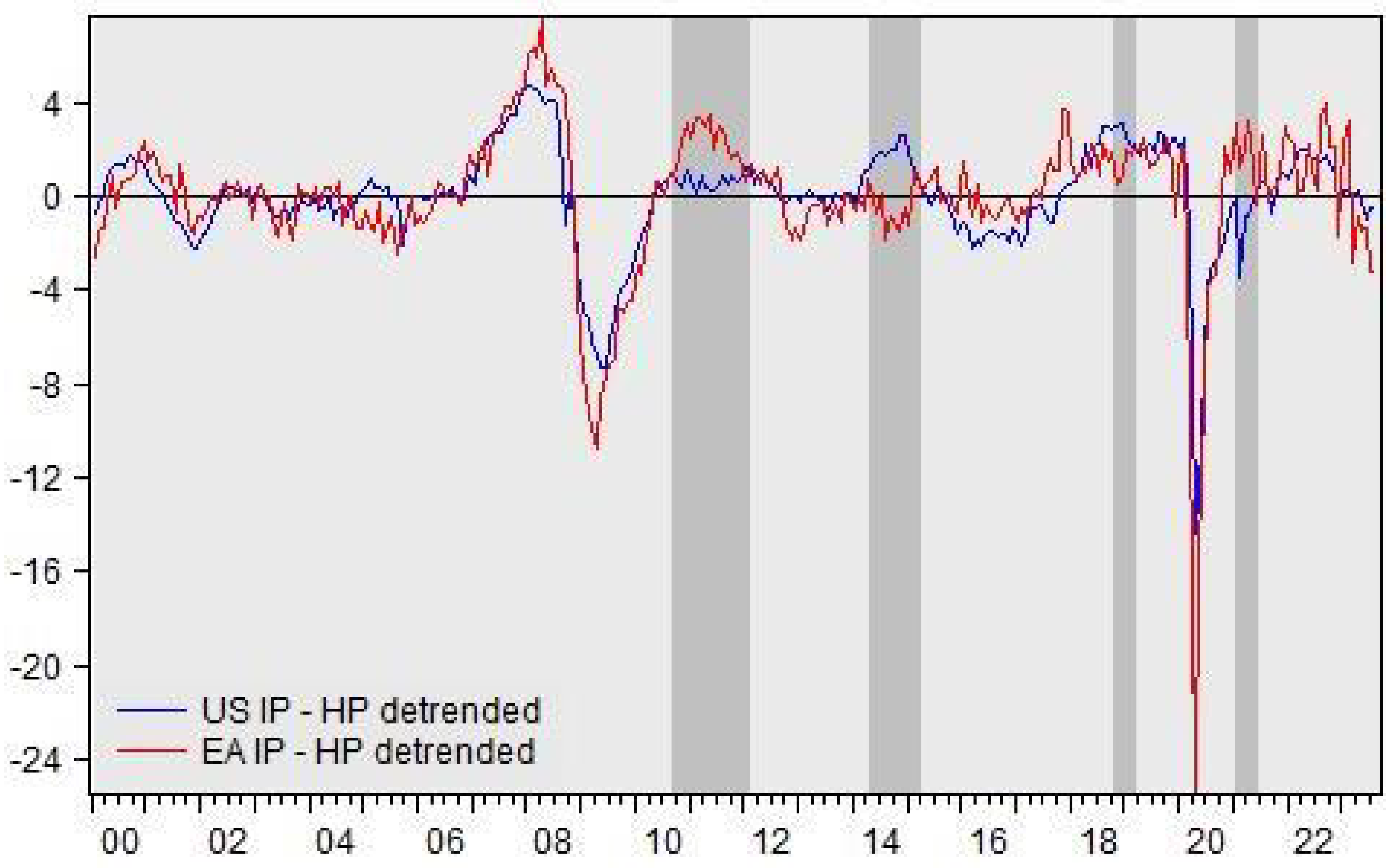
Figure 2 presents the HP-filtered industrial production indices of the US and Euro area. Eyeballing the figures, we can see that the indices followed a clear co-movement, except for the periods between 2010 and 2011, between mid-2014 and mid-2015, between late 2018 and early 2019, and between early 2021 and mid-2021. The first subperiod fell within Eurozone crisis; the second subperiod fell within the normalization period of the Fed, with a tremendous rise in economic growth, which was followed by a rise in the policy rate for the first time since the Great Financial Crisis (GFC), whereas, for the ECB, economic stagnation prevailed; the third subperiod fell within the last term of the normalization period, with a rise in the interest rate due to economic expansion in the US, whereas the Euro area went through economic contraction; and, lastly, the fourth sub-period reflected a recovery in the Euro area, whereas another economic downturn was visible following the COVID-19 pandemic.
As a summary of the two key macroeconomic indicators, we may argue that there was a leader role of the Fed regarding the policy rate but not during the entire period or some of the co-movement. We may argue that over time, the ECB has become much more assertive in its responses, aided by the requirements of the EU enlargement process that would expand the sovereignty of the monetary policy in the region. The adherence to the rules set by the Maastricht criteria following the entry to the monetary union added an important source of credibility to the ECB as the main guarantor of price stability.

4. Methodology

4.1. Measuring the Communication Tones

To measure the communication tones of the two CBs, we chose in-person contact with the public arguing that the physical presence of the presidents or the governors enhances the attention given by the public. Out of all possible communication tools, speeches, press conferences and testimonies (hearings), there are the main in-person contacts with the public3 that are closely watched by the stakeholders. For our purposes, we scraped all speeches, press conferences and hearings of the European Parliament from the ECB and all speeches, Federal Open Market Committee (FOMC) press conference transcripts and testimonies to the US Congress4 from the Fed between January 2000 and September 2023. The content of the press conferences of the FOMC was directly related to monetary policy, whereas speeches and testimonies covered a larger area of the economy such as exchange rates, fiscal policies, etc. Swanson (2023) highlighted the importance of the speeches and testimonies of the Fed compared to FOMC announcements, which take place as press releases. There is also a branch of literature focusing on the verbal communication of the CBs (Anand et al., 2022; Gertler & Horvath, 2018; Jansen & De Haan, 2007; Ranaldo & Rossi, 2010; Rosa, 2011). Moreover, many studies have utilized in-person communication tools of the CBs to measure communication tones or sentiments5 (see (Anastasiou et al., 2023; Bohl et al., 2023; Ferrara & Angino, 2022; Hüpper & Kempa, 2023; Klejdysz & Lumsdaine, 2023; Parle, 2022; Szyszko et al., 2022)).
In the baseline model, we used speeches as the data source, which were the most frequent communication type. In the augmented model, press conference statements and hearings/testimonies were added. The sentiment scores from the finBERT and LM algorithms, the number of documents employed, and the date ranges are shown in Table 1. To measure the sentiments of the texts, the recent literature utilized natural language processing (NLP) algorithms under several approaches, such as lexicon-based, machine learning (ML)-based, deep learning (DL)-based, hybrid model, etc6. In this study, we employed the most frequently used methods to scale the sentiment of economic and financial texts, namely, lexicon-based and transformer-based algorithms. Lexicon-based algorithms measure sentiments by word-counting based on the selected dictionary, whereas transformer-based algorithms measure the sentiment of each sentence based on the selected trained texts, such as financial texts. For the lexicon-based algorithm, we used the Loughran and McDonald (2011) Master Dictionary (1993–2021), hereafter LM. For the transformer-based algorithm, we used FinBERT.

4.1.1. LM Lexicon

Lexicon-based algorithms utilize a specific dictionary that classifies words into different sentiments such as positive, negative, neutral, etc. Basically, sentiment scores are measured following the word-counting of the relevant categories. There are many lexicons used in the literature. The literature measuring CB communication tones uses the LM lexicon heavily for general sentiment (Anastasiou et al., 2023; Bohl et al., 2023; Hayo & Zahner, 2023; Klejdysz & Lumsdaine, 2023; Szyszko et al., 2022; Yu et al., 2023). Therefore, for the content of the CB communication tools, we employed the LM lexicon to measure the general tone of the two CBs.
In the lexicon-based algorithm, we employed the “rvest” R-package for textual mining and the “tm” and “NLP” R-packages for sentiment analysis. Before tone measurement, we applied some transformations on the original data. We removed unwanted symbols, punctuations, numbers and stop words. Then, we constructed the Document-Term Matrix, which was a NxM matrix where N was the number of speech documents and M was the number of single words in the speech documents. In our approach, our aim was not to distinguish terms such as “high inflation” and “low unemployment”, where the single word “high” (“low”) referred to a positive/hawkish (negative/dovish) tone, whereas “high inflation” (“low unemployment”) as a term referred to a negative (positive) tone. As such, using compound words did not help us measure the tone, independent of the message carried in the speech itself. The general tone was measured via the P W N W P W + N W formula, where PW and NW indicated positive and negative words counts, respectively. In a simple manner, according to the chosen dictionary, the total number of negative words were deducted from the total positive words given the overall text and divided by the summation of the negative and positive words, providing an index between −1 and 1. The tone variables were converted into a monthly frequency by arithmetic averaging.

4.1.2. FinBERT

Following the developments in the computational linguistics, large language models (LLMs) were created using ML and DL methods that took into account the grammar and order of the words via a learning process based on initial training on an enormous textual dataset.
Approaches based on ML utilize models trained on extensive labeled datasets to detect patterns in text and generalize these insights to new data. Among the various algorithms available, transformer-based models are particularly popular. A notable example is BERT (Bidirectional Encoder Representations from Transformers) by Google, which, after fine-tuning, is highly effective for sentiment analysis. BERT operates as a multi-layer deep learning framework, starting with an encoder that processes input text and concluding with an output layer designed to classify sentiment as positive, negative or neutral. Huang et al. (2023) introduced FinBERT, which is a form of bidirectional encoder representations from transformers (BERT) and DL-based NLP algorithms, customized for financial texts. FinBERT provides the likelihood of positive, negative and neutral sentiments, which is measured for each sentence within each document. Positive ( P o s i t ) , negative ( N e g i t ) and neutral ( N e u i t ) sentiment scores are the probabilities of positive, negative or neutral categories ( C p o s , C n e g and C n e u , respectively) given the sentence ( S i t ) , where i presents each sentence and t presents the timestamp of each document.
P ( C p o s | S i t ) + P ( C n e g | S i t ) + P ( C n e u | S i t ) = 1
To obtain the sentiment score of the overall document, we calculated positive and negative normalized positive intensities, i.e., positive sentiment intensity ( P S I ) and negative sentiment intensity ( N S I ):
P S I t = i = 1 N P o s i t N
N S I t = i = 1 N N e g i t N
where N is the total number of sentences in each document. We could calculate the overall tone by deducting negative sentiment intensity from positive sentiment intensity:
T o n e t = P S I t N S I t
For each sentence, sentiment scores were calculated and averages of these probabilities according to the total number of sentences provided the intensity of the sentiments. For instance, in a FED speech regarding remarks on the economy and monetary policy7, the positive, negative and neutral probabilities were 0.999, 0 and 0 for the first sentence; 0, 0.742 and 0.258 for the second sentence; and, 0, 0.998 and 0.002, respectively, for the third sentence, as given in Table 2. The averages of the positive, negative and neutral probabilities of the first three sentences were 0.33, 0.58 and 0.09, respectively. In other words, these values were the positive, negative and neutral sentiment intensities under the assumption that there were 3 sentences in this speech. Accordingly, T o n e was calculated as the deduction of N S I , i.e., 0.58, from P S I , i.e., 0.33, which gave a value of −0.25 in this example.
Before calculating the finBERT score, we filtered out documents using languages other than English. We employed the “reticulate” R-package and imported “transformers” and “torch” libraries and “yiyanghkust/finbert-tone” models for sentiment analysis. As for pre-processing, we applied a minimal procedure by truncating sentences to 512 tokens as a basic method of sentence splitting.

4.2. Wavelet Coherence

Since the relationship between the variables of interest are not static, many empirical studies employ methodologies allowing for asymmetric behavior. Regression models allowing for nonlinearity can be helpful at a certain point but are not satisfactory when the relationship cannot be parameterized. At this point, nonparametric models step in by avoiding assumptions about the functional form, such as kernel smoothing, which conducts localization (focusing on a specific subset of the data) in time, or Fourier-based methods, which conducts localization in frequency. Relatively higher frequencies and longer-term horizon data are more susceptible to asymmetricity in both time and frequency dimensions. Wavelets capture both by decomposing the series into fractions of time (bringing information at specific time periods) and scale (inversely related to frequency, hence bringing information at low frequencies, such as trends, and high frequencies, i.e., details, simultaneously). Wavelets are also advantageous in denoising by using a significance level and handling non-stationary series by using a mother wavelet, which is an oscillatory function to localize time and frequency components. Among several continuous and discreet wavelets for wavelet transformation, Morlet wavelet is one of the most common as it performs best in capturing oscillations which is highly possible in financial data. On the other hand, in the presence of sharp spikes, Morlet wavelet may not be ideal, which may require a pre-processing. To filter out potentially available abrupt changes or spikes in the CB speech data, we used monthly averages of the higher frequency data. This gave us a balance in between measuring scales from details to trends and filtering out excess noise. Morlet wavelet was presented as follows:
φ ( η ) = π 1 / 4 e i w 0 η e η 2 / 2
where w 0 is a dimensionless frequency and η is dimensionless time with η = s . t , where s is the scale factor. i is the imaginary unit, i.e., i = 1 , which creates the oscillation. e η 2 / 2 refers to the Gaussian envelope and π 1 / 4 defines the phase shift. Given time series X with values of x n , where n = 1 , . . . , N (i.e., N is the number of points in the time series), Grinsted et al. (2004) defines the formula of continuous wavelet transform (CWT) as follows:
W n X ( s ) = δ t s n = 1 N x n φ [ ( n n ) δ t s ]
where δ t is the uniform time steps to ensure that the time series is sampled in discreet form, δ t s is the normalization factor and ( n n ) shows the difference between the position of a data point and the center of the wavelet.
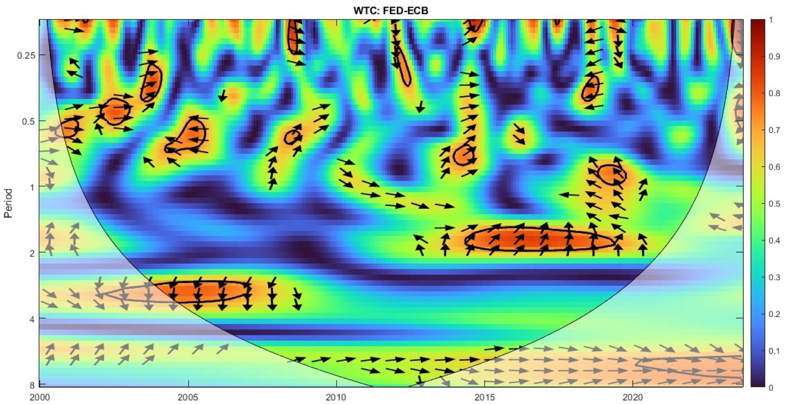
To examine the interdependence of the two CBs, we applied wavelet coherence (WTC) methodology8, which involves (i) wavelet coherence, which is similar to a traditional correlation in a localized form, to measure the strength of the relationship in the time frequency space; (ii) phase relationships to explore the lead/lag positions; (iii) the time domain, to take into account the time dynamics of the relationship; and (iv) the frequency domain, to interpret the relationship in terms of the frequency scale, such as short or long run.
To measure the WTC, the cross wavelet transform (XWT) of two time series, i.e., x n and y n , was measured by multiplying W n X and W n Y * , where (*) denotes complex conjugation. XWT captured common power and phase differences. Following Torrence and Webster (1999), wavelet coherence was defined as follows:
R n 2 ( s ) = | S ( s 1 W n X Y ( s ) ) | 2 S ( s 1 | W n X ( s ) | 2 ) S ( s 1 | W n Y ( s ) | 2 )
where S is the smoothing parameter. Wavelet coherence ( R n 2 ( s ) ), which was the absolute value squared of the smoothed cross-wavelet spectrum, was within the margin of 0 (no co-movement) and 1 (perfect co-movement). π / 2 represented a phase difference of one-quarter of a cycle. If R n 2 ( s ) ( 0 , π / 2 ) , the first variable led the second in-phase; if R n 2 ( s ) ( π / 2 , π ) , the first variable led the second anti-phase; if R n 2 ( s ) ( π , π / 2 ) , the second variable led the first anti-phase; and if R n 2 ( s ) ( π / 2 , 0 ) , the second variable led the first in-phase. The phase relationship was detected through the direction of the arrows. In our empirical analysis, the Fed was the first variable and the ECB was the second variable. Arrows pointing to the right denoted that the variables were in-phase, i.e., there was co-movement (in the same direction), whereas arrows pointing to the left denoted anti-phase (out of phase), i.e., movement in the opposite direction. Arrows pointing down and to the right indicated that the first variable led the in-phase, up and to the right indicated that the second variable led the in-phase, up and to the left indicated that the first variable led the anti-phase, and down and to the left indicated that the second variable led the anti-phase.
The significance level of the WTC was determined using Monte Carlo simulations; the 5% significance level is represented with a thick black outline that contains the red area (confidence area contour). The lighter shade under the thin black line that contains the cone of influence (COI) indicates an area that should be interpreted with caution since there were edge effects that might have distorted the picture.

5. Empirical Findings

This study utilized wavelet coherence methodology to investigate the interdependence of the communication tones of two CBs measured via sentiment analysis. Wavelet coherence analysis goes beyond regression models or Granger causality testing since it reveals information regarding co-movement and leader/follower patterns in varying time periods and frequency bands. As such, it is not limited to providing inference on a fixed environment in terms of time and the chosen frequency. Figure 3, Figure 4, Figure 5 and Figure 6 display the relationship between the two CBs involving time, frequency and wavelet coherence power using LM and finBERT algorithms using speeches and extended speeches of the two CBs. Right vertical axes display the wavelet coherence, which ranges in a color palette from dark blue (low values) to dark red (high values) according to the power. Left vertical axes display the scale bands, which range from the highest frequency (top of the left axis) to the lowest frequency (bottom of the left axis) and show the period in years. The highest frequency was one month and lowest frequency was 8 years9. Finally, the horizontal axis reflects the time period. Regarding the findings from the wavelet coherence, we disregarded the areas outside the significant region (red areas with a thick black outline) and outside the cone of influence (shaded region).

5.1. Wavelet Coherence for Speeches

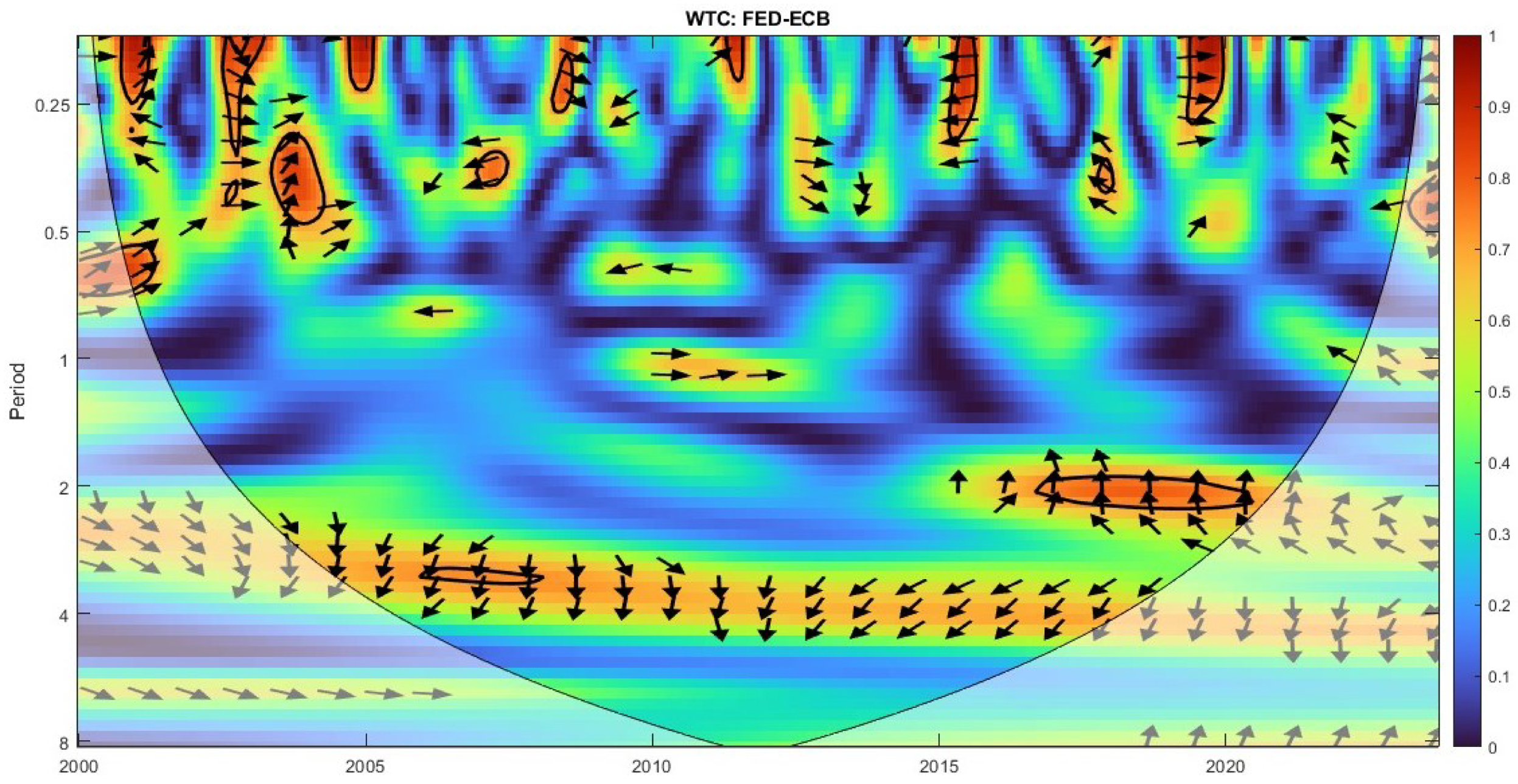
Regarding the LM-based approach, Figure 3 indicates that between mid-2000 and mid-2001, the Fed led the in-phase over 0–0.25 and 0.5–0.7 years of cycles; between mid-2002 and 2003, either the ECB led the in-phase or the two CBs comoved in the same direction over 0–0.45 years of cycles; between mid-2003 and mid-2004, the Fed led the in-phase over 0.3–0.5 years of cycles; between the end of 2006 and mid-2007, the ECB led the out-of-phase over 0.3–0.35 years of cycles; in 2008, the ECB led the in-phase over 0.1–0.3 years of cycles; in 2011, the Fed led the in-phase over 0–0.2 years of cycles; in 2015, the ECB led the out-of-phase over 0–0.4 years of cycles; between mid-2017 and 2016 the Fed leads out of phase over 0.4–0.45 years of cycles; and in 2019, either the two CBs co-moved in the same direction or the ECB led the in-phase over 0–0.3 years of cycles. These short-run findings suggest that the ECB had a leading role during 2002–2003, 2007–2008 and 2015. The year 2002 was a pivotal point for the ECB due to the physical launch of the euro. Accordingly, a leading role of the ECB could be expected, together with the rise in the communication with the public, to introduce the new currency. Moreover, the leading role of the ECB during the 2008 period was consistent with the financial crisis narrative of the US economy. During this period, the ECB increased its policy rate to maintain price stability, despite the concerns over economic stagnation, signaling a strong commitment to its primary mandate. Lastly, the 2015 period also stood out as period of the full-scale implementation of the QE to fight the prolonged period of low inflation. Moreover, the opposite directions of the two CBs was also consistent during that period since the Fed applied a contractionary monetary policy for the first time since the crisis. Regarding the leading role of the Fed in the short run, wavelet analysis pointed to the 2000–2001, 2003–2004, 2011 and 2017–2018 periods. The period up until 2006 was the Greenspan era of the Fed, which stood out as an influential governor with the longest official economic expansion in US history. Several studies highlight the strong communication skills of Greenspan (Bligh & Hess, 2007; El-Shagi & Jung, 2015; Mishkin, 2005) despite his vague rhetoric. Accordingly, a global leading role of the Fed was expected, excepting the ECB’s rise in communication during certain periods such as the physical introduction of the euro. During the period 2011, with a sovereign debt crisis in the countries of the South-West Euro Area Periphery (Portugal, Ireland, Italy, Greece and Spain), ECB’s communication tone became less powerful, which may have led to the dominance of the Fed. The 2017–2018 period also showed opposite direction paths for the two CBs, but this time with the Fed’s leading role. During this period, the Fed continued tightening its monetary policy, whereas the ECB continued QE. The different era of the two CBs appeared to create a divergence in their tones. Overall, in the short run, there was no clear dominance of any of the CBs. Hilscher et al. (2024), using a regression model with lagged regressors, observed a negative impact of the ECB on the Fed in the short run but not vice versa. In this respect, regression analysis failed to capture a relationship that could change over the time horizon and frequency. In this sense, the methodological contribution of wavelet analysis becomes clear.
Besides the significant regions in the short run, there were two significant regions in the medium run;: (i) between 2006 and 2008, the ECB led the out-of-phase over around 3.5 years of cycles, and (ii) between mid-2016 and mid-2020, the Fed led either the in-phase or out-of-phase over 2–2.5 years of cycles. The first region coincided with the mixed period (contractionary, steady and expansionary policy rate in order) of the Fed due to rising inflation risks and then the recession of the US economy and the contractionary monetary policy period of the ECB. For this period, wavelet coherence analysis depicted a leading role of the ECB but in an opposite direction. The second region again coincided with the mixed period (contractionary, steady and expansionary policy rate in order) of the Fed and the ECB’s main refinancing operations (MROs) hitting the 0% level period for the first time ever with large-scale quantitative easing. We could argue that the QE period of the ECB to increase inflation back to the 2% target level and revive the economy diminished the international effectiveness of the ECB by pursuing more domestic-oriented policies. Moreover, during this period, the Fed applied more assertive policies, which went together with the high growth rate before the COVID-19 pandemic. Last but not least, there seemed to be no significant region in the long run (below around period 4). Figure A1a of Appendix A shows the long-run trend of the LM lexicon using HP filtering. Eyeballing this, we could argue that there was no co-movement regarding the long-run trends of the two CBs.
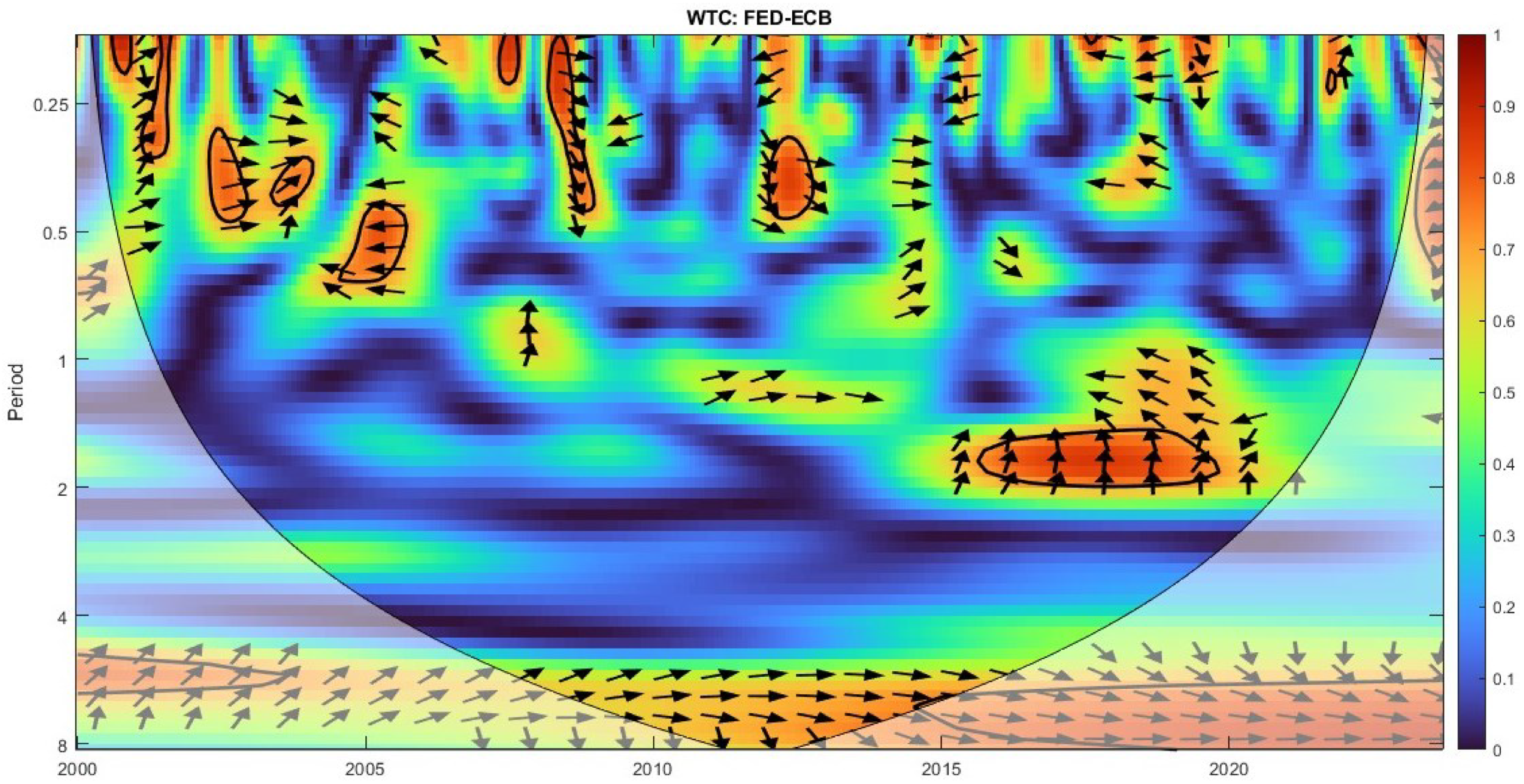
Regarding the finBERT approach, Figure 4 indicates that in 2001, the Fed led the in-phase over 0–0.24 years of cycles; in 2002, either the ECB or the Fed led the in-phase over 0.3–0.5 years of cycles; in 2003, the Fed led the in-phase over 0.3–0.4 years of cycles; between mid-2004 and mid-2005, the two CBs moved in the opposite direction over 0.4–0.7 years of cycles; in 2008, the ECB led the in-phase over 0–0.5 years of cycles; and, finally, in 2012, the ECB led the in-phase over 0.3–0.5 years of cycles. The leading role of the ECB during 2002 and the 2008 period in the short run was similar to that of the LM lexicon. Moreover, the leading role of the ECB during 2012 was in line with Mario Draghi’s famous “whatever it takes” speech that underlined the strong stance to preserve the euro. Besides the significant regions in the short run, there was one significant region in the medium run: between mid-2016 and 2019, the Fed led either the in-phase or out-of-phase over 1.8–2.1 years of cycles. This clear leading role of the Fed was also observed in the LM lexicon, highlighting the passive and internal-politics era of the ECB and the assertive and growing era of the Fed. Last but not least, there were two significant regions in the long run; between 2000 and 2003 and post-2015; however, they were inside the COI. Figure A1b of Appendix A shows the long-run trend of finBERT using HP filtering. Eyeballing this, there seems to be a co-movement in the shaded region, similar to the long-run result of the wavelet analysis.
After the inspection of the two wavelet coherence figures using LM and finBERT methods, a clear similarity in terms of the direction and lead/lag effects was observed in the medium run between 2016 and 2019. There were minor similarities during 2002 and 2008 in the short run; however, no similarity was captured in the long run. This finding suggests that the two methodologies, LM and finBERT, which are positioned in different contexts in the literature, are in fact not very diverse from each other, especially in the medium run. We managed to identify this observation by decomposing the relationship in terms of the frequency domain. Hence, wavelet analysis revealed its technical contribution as a methodology by decomposing the co-movement or lead/lag effects over the frequency domain.

5.2. Robustness Check: Wavelet Coherence for Extended Speeches

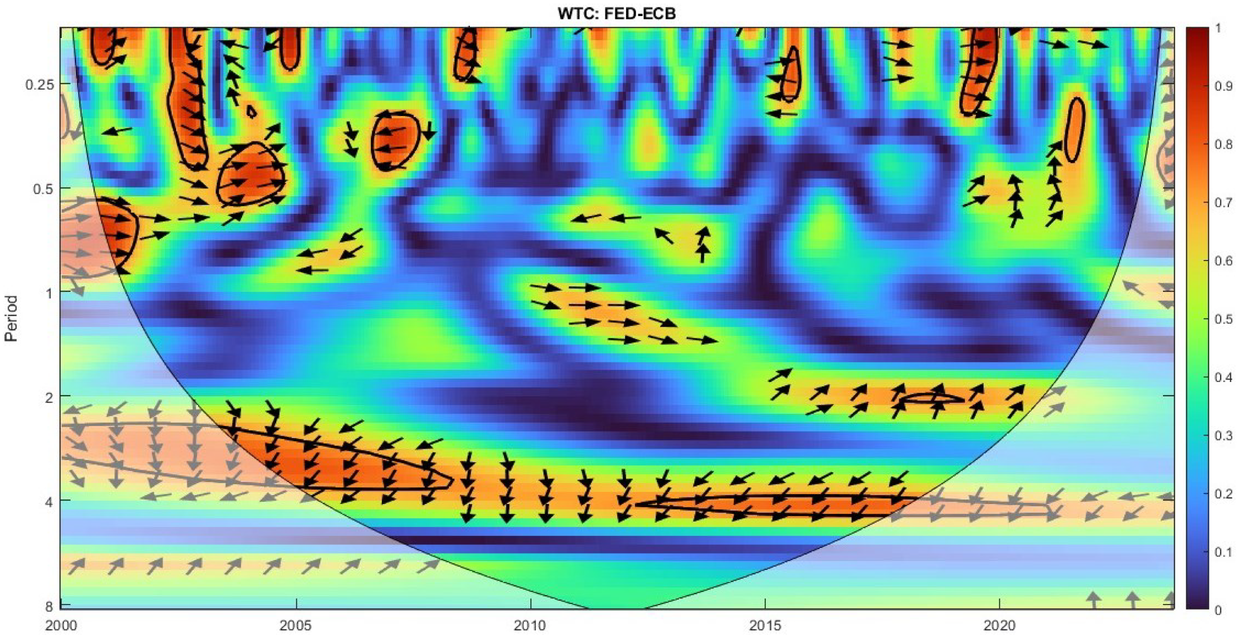
After the speeches, we employed extended speeches as a robustness check of the two CBs. An initial observation was that the wavelet visualization for the extended speech was similar to the visualization for the speech in the short run. Regarding the LM, Figure A1a shows that between mid-2000 and mid-2001, the Fed led the in-phase over 0–0.2 years of cycles and there was either a leading role of the Fed or an ECB in-phase over 0.5–0.8 years of cycles; in 2002, the ECB led the in-phase over 0–0.45 years of cycles; between mid-2003 and mid-2004, the Fed led the in-phase over 0.3–0.6 years of cycles; between the end of 2006 and mid-2007, the ECB led the out-of-phase over 0.3–0.4 years of cycles; in 2008, the ECB led the in-phase over 0–0.25 years of cycles; in 2015, the Fed led the out-of-phase over 0–0.3 years of cycles; in 2019, either the two CBs co-moved in the same direction or the ECB led the in-phase over 0–0.35 years of cycles. The leading roles of the ECB and the Fed in the short run during certain periods were consistent with the LM lexicon results obtained using the speeches. Besides the significant regions in the short run, there were two significant regions in the medium run: (i) between mid-2003 and 2008, the ECB led the out-of-phase over 2.5–3.5 years of cycles, and (ii) between mid-2017 and mid-2019, the Fed led the in-phase over around 2 years of cycles. The leading role of the ECB was also similar to that of the LM lexicon when using the speeches. However, the second significant region reflected a leading role of the Fed in the same direction, which was either in-phase or out-of-phase in the LM lexicon results when using the speeches. Last but not least, there seemed to be a significant region between 2013 and 2020 in the long run (below around period 4). Figure A1c of Appendix A also shows the long-run trend of the LM lexicon using HP filtering. Eyeballing this, we could argue that there seems to be a co-movement in the shaded region, similar to the long-run result of the wavelet analysis.
Regarding finBERT, Figure A1d indicates a leading role of either the Fed or the ECB for the in-phase between mid-2000 and mid-2001 over 0.5–0.6 years of cycles and in 2002 over 0.4–0.6 years of cycles; in 2003, the Fed led the in-phase over 0.3–0.45 years of cycles; between 2004 and mid-2005, either the Fed led the out-of-phase or the two CBs moved in the opposite direction over 0.5–0.7 years of cycles; in 2008, the ECB led the in-phase over 0–0.25 years of cycles and the Fed led the in-phase over 0.5–0.6 years of cycles; in 2012, the ECB led the in-phase over 0.3–0.5 years of cycles; in 2014, the Fed led the in-phase over 0–0.15 and 0.8–0.9 years of cycles; and in 2018, the ECB led the out-of-phase over 0.3–0.4 years of cycles. During 2003 and 2008 in the short run, the leading roles of the ECB and the Fed were similar to the LM results for the extended speeches. Besides the significant regions in the short run, there were two significant regions in the medium run: (i) between mid-2003 and 2007, the ECB led the out-of-phase over 2.5–3.5 years of cycles, and (ii) between mid-2014 and mid-2019, the Fed led the in-phase over around 2 years of cycles. These findings showed clear signs of similarities between the two algorithms in the medium run. Last but not least, there was one significant region in the long run after 2020; however, it was inside the COI. Figure A1b of Appendix A also shows the long-run trend of finBERT using HP filtering. Eyeballing the evidence, we could argue that there is a co-movement in the shaded region, similar to the long-run result of the wavelet analysis.
As shown in the two wavelet coherence figures produced using the LM and finBERT methods, the similarity in terms of the direction and lead/lag effects persisted in the medium run between mid-2003 and 2007 and between mid-2017 and mid-2019; there was a minor similarity during the periods of 2003 and 2008 in the short run; however, no similarity was captured in the long run.

6. Conclusions

In this study, we shed light on the leader/follower roles and their relationship by analyzing the communication tones of the speeches delivered by the two CBs using wavelet coherence analysis. The tones were measured by two prominent algorithms and significant regions for both algorithms were compared for similarity. Our findings suggest that there was no static leading role assigned either to the Fed or the ECB; on the contrary, the leading role changed over the time horizon. This dynamic relationship was also observed in terms of the frequency dimension such that the leading role varied over the frequency domain. Using wavelet coherence analysis, the dynamic relationship between the two CBs over the two dimensions was identified. Last but not least, we compared wavelet coherence visualizations between the LM lexicon and finBERT scores. A visual inspection shows that there were some minor similarities in the short run and major similarities in the medium run, a result that offers support to the LM lexicon approach as a useful complementary tool to transformer-based alternatives.
The findings regarding the medium run show the leading role of the ECB during the (pre-)crisis period of the US and the leading role of the Fed during the QE period of the ECB. Accordingly, we could argue that the GFC crisis affected the Fed losing its leadership, whereas reviving inflation back to the target level affected the ECB losing its leadership. This finding is, in a way, in line with the study of Bohl et al. (2023), which suggested that unemployment expectations in the Fed speeches ande inflation expectations in the ECB speeches influenced their tone. The findings in the medium run seem to be consistent with the narrative of the macroeconomic dynamics for both CBs. Our findings underscore the importance of counter-cyclical leadership, such that CBs may undertake proactive communication roles during the periods that their counterpart is facing economic challenges. Strong and confident language used by a leading CB may help mitigate potential spillover effects and maintain stability in global money markets. Moreover, it was observed that the independence of the communication tones, depicted by the blue area, was very common in the wavelet coherence visualizations. This suggests the relatively different communication strategies followed by the two CBs. In conclusion, we can argue that this examination of the interdependence of the communication tones of the two CBs is informative.

Author Contributions

Methodology, P.D. and T.S.; software, P.D. and T.S.; formal analysis, P.D. and T.S.; writing—original draft preparation, P.D. and T.S.; writing—review and editing, P.D. and T.S.; visualization, P.D. and T.S. All authors have read and agreed to the published version of the manuscript.

Funding

This research received no external funding.

Institutional Review Board Statement

Not applicable.

Informed Consent Statement

Not applicable.

Data Availability Statement

Data will be made available upon request.

Conflicts of Interest

The authors declare no conflicts of interest.

Appendix A. Long-Run Trends of the Lexicons
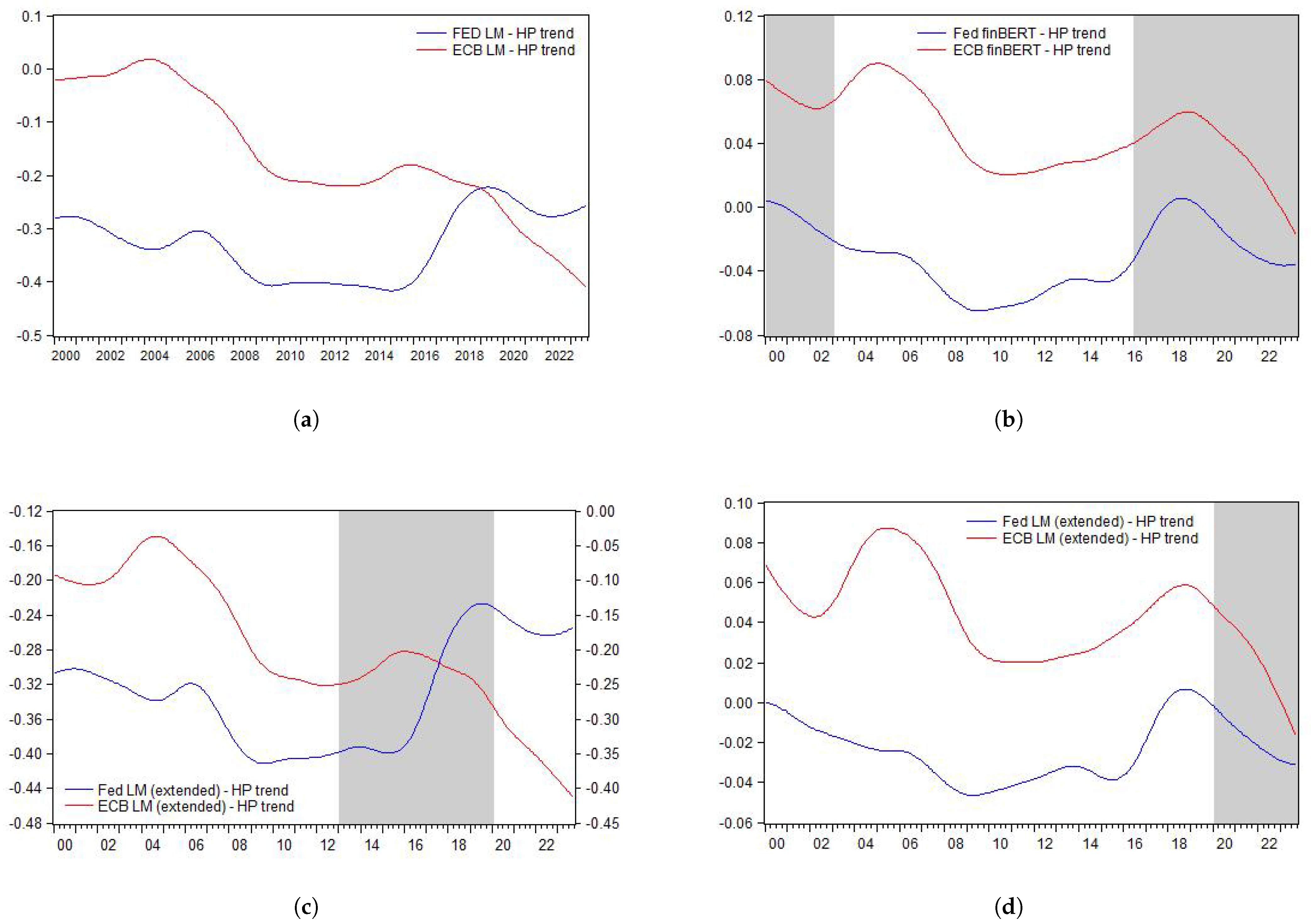
Figure A1. Long-run trends of LM and finBERT algorithms. (a) LM lexicon (speeches). (b) finBERT (speeches). (c) LM lexicon (extended speeches). (d) finBERT (extended speeches).
Jrfm 18 00191 g0a1

Notes

1
One relatively recent example to highlight the importance of the communication of the central banks is the public statements made several times by the ECB president, Jean-Claude Trichet, disregarding the impact of the US monetary policies on the Eurozone (Willard & Vidaillet, 2009).
2
While examining the relationship between the two CBs, regression models will neglect the dynamic structure of the relationship between two CBs, which are even dynamic as themselves. For example, Swanson (2023) mentions the change in the importance of the Fed speeches over time. Regarding the interdependence of the two CBs, Vukovic et al. (2021) apply wavelet coherence using money market returns with different maturities using interbank rates and bond returns for the period 2004–2018 taking into account the frequency domain of the relationship
3
There are some other communication tools, however they are discarded from the analysis due to their low frequency.
4
5
Szyszko et al. (2022) mention about the differences between the tone and the sentiment in the monetary policy literature such that sentiments are the unpredictable component of the tone.
6
NLP is a subfield of artificial intelligence to analyze human language and text pre-processing part of NLP helps clean and prepare the text. ML is the learning process of the machines from the patterns in the data. DL is a subset and more comprehensive version of ML that mimics the learning process of the brain and helps process unstructured data such as texts, images, etc.
7
8
We use the Matlab package of Grinsted et al. (2004).
9
We may assume period 1 as a threshold to divide short run (values lower than 1) and long run (values higher than 1) findings.

References

  1. Anand, A., Basu, S., Pathak, J., & Thampy, A. (2022). Whose speeches impact European markets: ECB’s or the national central banks’? European Financial Management, 28(5), 1413–1476. [Google Scholar] [CrossRef]
  2. Anastasiou, D., Krokida, S.-I., Tsouknidis, D., & Drakos, K. (2023). Can the tone of central bankers’ speeches discourage potential bank borrowers in the Eurozone? Journal of International Money and Finance, 139, 102950. [Google Scholar]
  3. Apel, M., & Grimaldi, M. B. (2014). How informative are central bank minutes? Review of Economics, 65(1), 53–76. [Google Scholar]
  4. Bailey, A., & Schonhardt-Bailey, C. (2008). Does deliberation matter in FOMC monetary policymaking? The Volcker Revolution of 1979. Political Analysis, 16(4), 404–427. [Google Scholar]
  5. Batten, D. S., & Ott, M. (1985). The interrelationship of monetary policies under floating exchange rates: Note. Journal of Money, Credit and Banking, 17(1), 103–110. [Google Scholar]
  6. Belke, A., & Cui, Y. (2010). US–Euro area monetary policy interdependence: New evidence from Taylor rule-based vecms. World Economy, 33(5), 778–797. [Google Scholar]
  7. Belke, A., & Gros, D. (2005). Asymmetries in transatlantic monetary policy-making: Does the ECB follow the fed? JCMS: Journal of Common Market Studies, 43(5), 921–946. [Google Scholar] [CrossRef]
  8. Bennani, H., & Neuenkirch, M. (2017). The (home) bias of European central bankers: New evidence based on speeches. Applied Economics, 49(11), 1114–1131. [Google Scholar] [CrossRef]
  9. Bergin, P. R., & Jordà, Ò. (2004). Measuring monetary policy interdependence. Journal of International Money and Finance, 23(5), 761–783. [Google Scholar]
  10. Bjerkander, L., & Glas, A. (2024). Talking in a language that everyone can understand? Clarity of speeches by the ECB Executive Board. Journal of International Money and Finance, 149, 103200. [Google Scholar]
  11. Bligh, M. C., & Hess, G. D. (2007). The power of leading subtly: Alan Greenspan, rhetorical leadership, and monetary policy. The Leadership Quarterly, 18(2), 87–104. [Google Scholar]
  12. Blinder, A. S., Ehrmann, M., De Haan, J., & Jansen, D.-J. (2024). Central bank communication with the general public: Promise or false hope? Journal of Economic Literature, 62(2), 425–457. [Google Scholar]
  13. Blinder, A. S., Ehrmann, M., Fratzscher, M., De Haan, J., & Jansen, D.-J. (2008). Central bank communication and monetary policy: A survey of theory and evidence. Journal of Economic Literature, 46(4), 910–945. [Google Scholar]
  14. Bohl, M. T., Kanelis, D., & Siklos, P. L. (2023). Central bank mandates: How differences can influence the content and tone of central bank communication. Journal of International Money and Finance, 130, 102752. [Google Scholar]
  15. Burdekin, R. C. (1989). International transmission of US macroeconomic policy and the inflation record of Western Europe. Journal of International Money and Finance, 8(3), 401–423. [Google Scholar]
  16. Burdekin, R. C., & Burkett, P. (1992). The impact of US economic variables on bank of Canada policy: Direct and indirect responses. Journal of International Money and Finance, 11(2), 162–187. [Google Scholar]
  17. Canzoneri, M. B., & Gray, J. A. (1985). Monetary policy games and the consequences of non-cooperative behavior. International Economic Review, 547–564. [Google Scholar]
  18. Chung, J. W. (1993). Monetary interdependence among G-3 countries. Applied Economics, 25(5), 681–688. [Google Scholar]
  19. de Haan, J., & Hoogduin, L. (2024). ECB communication policies: An overview and comparison with the Federal Reserve. Journal of International Money and Finance, 103050. [Google Scholar]
  20. de Haan, J., Jansen, D.-J., & de Haan, J. (2007). The importance of being vigilant: Has ecb communication influenced euro area inflation expectations? (Tech. Rep.). CESifo. [Google Scholar]
  21. Devereux, M. B., & Engel, C. (2003). Monetary policy in the open economy revisited: Price setting and exchange-rate flexibility. The Review of Economic Studies, 70(4), 765–783. [Google Scholar]
  22. Dominguez, K. M. (1998). Monetary interdependence and coordination. SSRN. [Google Scholar]
  23. Dybowski, T. P., & Kempa, B. (2020). The European Central Bank’s monetary pillar after the financial crisis. Journal of Banking & Finance, 121, 105965. [Google Scholar]
  24. Ehrmann, M., & Fratzscher, M. (2002). Interdependence between the euro area and the US: What role for EMU? (Available at SSRN 376184). European Central Bank. [Google Scholar]
  25. Ehrmann, M., & Fratzscher, M. (2005). Equal size, equal role? Interest rate interdependence between the euro area and the United States. The Economic Journal, 115(506), 928–948. [Google Scholar] [CrossRef]
  26. Eijffinger, S. C. (2008). How much inevitable US-Euro Area interdependence is there in monetary policy? Intereconomics, 43(6), 341–348. [Google Scholar] [CrossRef]
  27. El-Shagi, M., & Jung, A. (2015). Does the Greenspan era provide evidence on leadership in the FOMC? Journal of Macroeconomics, 43, 173–190. [Google Scholar] [CrossRef]
  28. Ferrara, F. M., & Angino, S. (2022). Does clarity make central banks more engaging? Lessons from ECB communications. European Journal of Political Economy, 74, 102146. [Google Scholar] [CrossRef]
  29. Galán Figueroa, J., & Villalba Padilla, F. I. (2022). Coordination and monetary policy among central banks. The NAFTA Case. Revista Economía y Política, 36, 45–66. [Google Scholar] [CrossRef]
  30. Gertler, P., & Horvath, R. (2018). Central bank communication and financial markets: New high-frequency evidence. Journal of Financial Stability, 36, 336–345. [Google Scholar] [CrossRef]
  31. Grinsted, A., Moore, J. C., & Jevrejeva, S. (2004). Application of the cross wavelet transform and wavelet coherence to geophysical time series. Nonlinear Processes in Geophysics, 11(5/6), 561–566. [Google Scholar] [CrossRef]
  32. Hamada, K. (1974). Alternative exchange rate systems and the interdependence of monetary policies. In National monetary policies and the international financial system. University of Chicago Press. [Google Scholar]
  33. Hamada, K. (1979). Macroeconomic strategy and coordination under alternative exchange rates. In International Economic Policy (pp. 292–324). Johns Hopkins University Press. [Google Scholar]
  34. Hayo, B., Henseler, K., Rapp, M. S., & Zahner, J. (2022). Complexity of ECB communication and financial market trading. Journal of International Money and Finance, 128, 102709. [Google Scholar] [CrossRef]
  35. Hayo, B., & Zahner, J. (2023). What is that noise? Analysing sentiment-based variation in central bank communication. Economics Letters, 222, 110962. [Google Scholar] [CrossRef]
  36. Heinemann, F., & Ullrich, K. (2007). Does it pay to watch central bankers’ lips? The information content of ECB wording. Swiss Journal of Economics and Statistics, 143, 155–185. [Google Scholar] [CrossRef]
  37. Hilscher, J., Nabors, K., & Raviv, A. (2024). Information in central bank Sentiment: An analysis of fed and ECB communication. (Available at SSRN 4797935). Available online: https://ssrn.com/abstract=4797935 (accessed on 1 February 2025).
  38. Huang, A. H., Wang, H., & Yang, Y. (2023). FinBERT: A large language model for extracting information from financial text. Contemporary Accounting Research, 40(2), 806–841. [Google Scholar]
  39. Hüpper, F., & Kempa, B. (2023). Inflation targeting and inflation communication of the Federal Reserve: Words and deeds. Journal of Macroeconomics, 75, 103497. [Google Scholar] [CrossRef]
  40. Jansen, D.-J., & De Haan, J. (2007). Were verbal efforts to support the euro effective? A high-frequency analysis of ECB statements. European Journal of Political Economy, 23(1), 245–259. [Google Scholar]
  41. Kahveci, E., & Odabaş, A. (2016). Central banks’ communication strategy and content analysis of monetary policy statements: The case of Fed, ECB and CBRT. Procedia-Social and Behavioral Sciences, 235, 618–629. [Google Scholar] [CrossRef]
  42. Kaminskas, R., & Jurkšas, L. (2024). ECB communication sentiments: How do they relate to the economic environment and financial markets? Journal of Economics and Business, 13, 106198. [Google Scholar]
  43. Klejdysz, J., & Lumsdaine, R. L. (2023). Shifts in ECB Communication: A textual analysis of the press conference. International Journal of Central Banking, 19(2), 473–542. [Google Scholar]
  44. Kokab, S. T., Asghar, S., & Naz, S. (2022). Transformer-based deep learning models for the sentiment analysis of social media data. Array, 14, 100157. [Google Scholar]
  45. Kotelnikova, A., Paschenko, D., Bochenina, K., & Kotelnikov, E. (2021, December 16–18). Lexicon-based methods vs. BERT for text sentiment analysis. International Conference on Analysis of Images, Social Networks and Texts (pp. 71–83), Tbilisi, GA, USA. [Google Scholar]
  46. Krampf, A. (2019). Monetary power reconsidered: The struggle between the Bundesbank and the fed over monetary leadership. International Studies Quarterly, 63(4), 938–951. [Google Scholar] [CrossRef]
  47. Laskar, D. (1986). International cooperation and exchange rate stabilization. Journal of International Economics, 21(1–2), 151–164. [Google Scholar]
  48. Lastra, R. M., & Dietz, S. (2022). Communication in monetary policy. Banking & Finance Law Review, 38, 365–403. [Google Scholar]
  49. Loughran, T., & McDonald, B. (2011). When is a liability not a liability? Textual analysis, dictionaries, and 10-Ks. The Journal of Finance, 66(1), 35–65. [Google Scholar]
  50. Mandler, M. (2010). Explaining ecb and fed interest rate correlation: Economic interdependence and optimal monetary policy. (Tech. Rep.). MAGKS Joint Discussion Paper Series in Economics. [Google Scholar]
  51. Mishkin, F. S. (2005). The Fed after Greenspan. Eastern Economic Journal, 31(3), 317–332. [Google Scholar]
  52. Möller, R., & Reichmann, D. (2021). ECB language and stock returns–A textual analysis of ECB press conferences. In The Quarterly Review of Economics and Finance (Volume 80, pp. 590–604). [Google Scholar]
  53. Obstfeld, M., & Rogoff, K. (2002). Global implications of self-oriented national monetary rules. The Quarterly Journal of Economics, 117(2), 503–535. [Google Scholar]
  54. Oudiz, G., Sachs, J., Blanchard, O. J., Marris, S. N., & Woo, W. T. (1984). Macroeconomic policy coordination among the industrial economies. Brookings Papers on Economic Activity, 1984(1), 1–75. [Google Scholar]
  55. Pappa, E. (2004). Do the ECB and the Fed really need to cooperate? Optimal monetary policy in a two-country world. Journal of Monetary Economics, 51(4), 753–779. [Google Scholar]
  56. Parle, C. (2022). The financial market impact of ECB monetary policy press conferences—A text based approach. European Journal of Political Economy, 74, 102230. [Google Scholar] [CrossRef]
  57. Picault, M., & Renault, T. (2017). Words are not all created equal: A new measure of ECB communication. Journal of International Money and Finance, 79, 136–156. [Google Scholar] [CrossRef]
  58. Ranaldo, A., & Rossi, E. (2010). The reaction of asset markets to Swiss National Bank communication. Journal of International Money and Finance, 29(3), 486–503. [Google Scholar] [CrossRef]
  59. Romer, C. D., & Romer, D. H. (1989). Does monetary policy matter? A new test in the spirit of Friedman and Schwartz. NBER Macroeconomics Annual, 4, 121–170. [Google Scholar]
  60. Rosa, C. (2011). Words that shake traders: The stock market’s reaction to central bank communication in real time. Journal of Empirical Finance, 18(5), 915–934. [Google Scholar]
  61. Rosa, C., & Verga, G. (2007). On the consistency and effectiveness of central bank communication: Evidence from the ECB. European Journal of Political Economy, 23(1), 146–175. [Google Scholar]
  62. Rosa, C., & Verga, G. (2008). The impact of central bank announcements on asset prices in real time. Thirteenth issue (June 2008) of the International Journal of Central Banking, 4(2), 175–217. [Google Scholar]
  63. Schmeling, M., & Wagner, C. (2016). Does central bank tone move asset prices? Journal of Financial and Quantitative Analysis, 60(1), 36–67. [Google Scholar]
  64. Scotti, C. (2006). A bivariate model of Fed and ECB main policy rates. FRB International Finance Discussion Paper No. 875. Available online: https://ssrn.com/abstract=953025 (accessed on 14 January 2025).
  65. Shapiro, A. H., & Wilson, D. J. (2022). Taking the fed at its word: A new approach to estimating central bank objectives using text analysis. The Review of Economic Studies, 89(5), 2768–2805. [Google Scholar]
  66. Svensson, L. E. (2006). The instrument-rate projection under inflation targeting: The norwegian example. Center for Economic Policy Studies, Princeton University. [Google Scholar]
  67. Swanson, E. T. (2023). The importance of fed chair speeches as a monetary policy tool. AEA Papers and Proceedings, 113, 394–400. [Google Scholar]
  68. Szyszko, M., Rutkowska, A., & Kliber, A. (2022). Do words affect expectations? The effect of central banks communication on consumer inflation expectations. The Quarterly Review of Economics and Finance, 86, 221–229. [Google Scholar]
  69. Tetik, M. (2020). Testing of leader-follower interaction between fed and emerging countries’ central banks. The Journal of Economic Asymmetries, 22, e00181. [Google Scholar]
  70. Torrence, C., & Webster, P. J. (1999). Interdecadal changes in the ENSO–monsoon system. Journal of Climate, 12(8), 2679–2690. [Google Scholar]
  71. Ullrich, K. (2003). A comparison between the Fed and the ECB: Taylor rules. (ZEW Discussion Paper). Leibniz Centre for European Economic Research. [Google Scholar]
  72. Ullrich, K. (2008). Inflation expectations of experts and ECB communication. The North American Journal of Economics and Finance, 19(1), 93–108. [Google Scholar]
  73. Vukovic, D. B., Lapshina, K. A., & Maiti, M. (2021). Wavelet coherence analysis of returns, volatility and interdependence of the US and the EU money markets: Pre & post crisis. The North American Journal of Economics and Finance, 58, 101457. [Google Scholar]
  74. Willard, A., & Vidaillet, T. (2009). Trichet says ECB considering more steps but U.S. different. [Newspaper Article, News on 18 March]. Reuters. Available online: https://www.reuters.com/article/business/trichet-says-ecb-considering-more-steps-but-u-s-different-idUSTRE52G78E/ (accessed on 10 January 2025).
  75. Wischnewsky, A., Jansen, D.-J., & Neuenkirch, M. (2021). Financial stability and the fed: Evidence from congressional hearings. Economic Inquiry, 59(3), 1192–1214. [Google Scholar]
  76. Yellen, J. (2005). The Yellen View, The International Economy Magazine. Available online: http://www.international-economy.com/TIE_Sp05_Yellen.pdf (accessed on 30 October 2024).
  77. Yu, Z., Liu, W., & Yang, F. (2023). A central bankers’ sentiment index of global financial cycle. Finance Research Letters, 57, 104161. [Google Scholar]
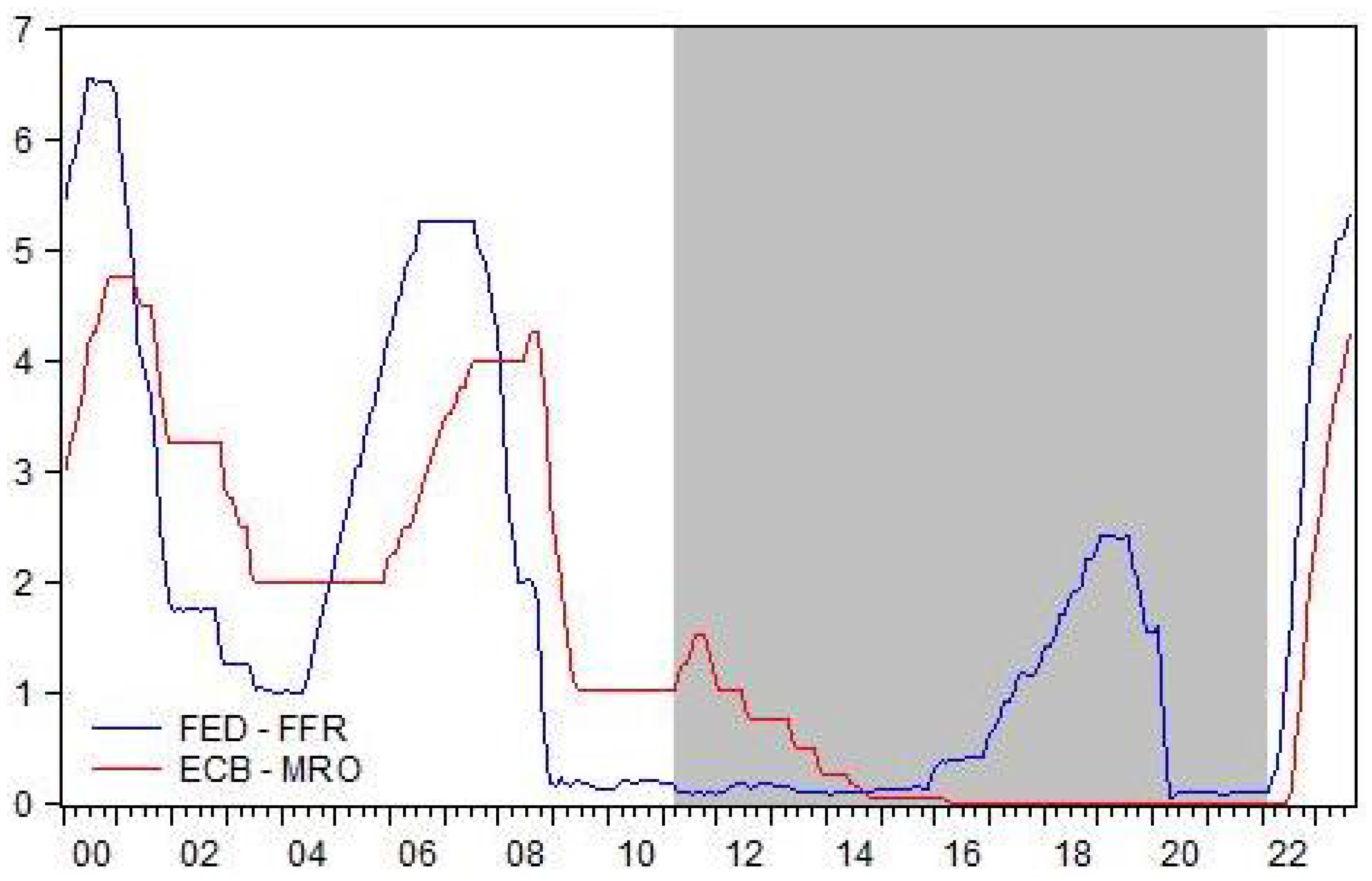
Figure 1. The Fed and the ECB policy rates (2000–2023). Note: Monthly averages of federal funds effective rate (FFR) and main refinancing operations (MROs) were used. The gray area provides a visual indication of a period with no co-movement.
Jrfm 18 00191 g001
Figure 2. The US and the Eurozone industrial production indices (2000–2023). Note: Monthly industrial production index (seasonally adjusted). The gray area provides a visual indication of a period with no co-movement.
Jrfm 18 00191 g002
Figure 3. WTC between the Fed and the ECB using LM for speeches.
Jrfm 18 00191 g003
Figure 4. WTC between the Fed and the ECB using finBERT for speeches.
Jrfm 18 00191 g004
Figure 5. WTC between the Fed and the ECB using LM for extended speeches.
Jrfm 18 00191 g005
Figure 6. WTC between the Fed and the ECB using finBERT for extended speeches.
Jrfm 18 00191 g006
Table 1. Descriptive statistics.
FedECB
Speech Conf Testimony Speech Conf Hearing
FinBERT
Mean−0.032−0.0430.0150.0460.0090.081
Std0.0480.0280.0740.0520.0530.080
Min−0.160−0.117−0.179−0.179−0.123−0.066
Max0.1490.0040.5000.2420.1310.284
LM
Mean−0.330−0.397−0.330−0.163−0.426−0.151
Std0.1660.0950.2190.1880.1200.187
Min−0.742−0.617−0.838−0.597−0.686−0.590
Max0.313−0.1220.3750.3980.0810.318
Obs2857018728524299
Date start01:200004:201101:200001:200003:200001:2000
Date end09:202309:202309:202309:202309:202309:2023
No. of docs1470713712244256102
Note: Conf is short for press conference.
Table 2. Example sentences for finBERT measurement.
Sentence Pos it Neg it Neu it
“The average pace of job gains over the past year has slowed somewhat and the labor force participation rate has also improved over the same time frame, a sign that labor market supply and demand may be coming into better balance”.0.99900
“Despite this tightening of bank lending standards, we have not seen signs of a sharp contraction in credit that would significantly slow economic activity”.00.7420.258
“This, along with my own expectation that progress on inflation is likely to be slow given the current level of monetary policy restraint, suggests that further policy tightening will be needed to bring inflation down in a sustainable and timely manner”.00.9980.002
Sentiment intensity0.330.580.09
Disclaimer/Publisher’s Note: The statements, opinions and data contained in all publications are solely those of the individual author(s) and contributor(s) and not of MDPI and/or the editor(s). MDPI and/or the editor(s) disclaim responsibility for any injury to people or property resulting from any ideas, methods, instructions or products referred to in the content.