Hedging via Perpetual Derivatives: Trinomial Option Pricing and Implied Parameter Surface Analysis

Abstract

We introduce a fairly general, recombining trinomial tree model in the natural world. Market completeness is ensured by considering a market consisting of two risky assets, a riskless asset and a European option. The two risky assets consist of a stock and a perpetual derivative of that stock. The option has the stock and its derivative as its underlying. Using a replicating portfolio, we develop prices for European options and generate the unique relationships between the risk-neutral and real-world parameters of the model. We discuss calibration of the model to empirical data in the cases in which the risky asset returns are treated as either arithmetic or logarithmic. From historical price and call option data for select large cap stocks, we develop implied parameter surfaces for the real-world parameters in the model.

1. Introduction

Despite known limitations—log-normal prices driven by Brownian motion; absence of the drift term of the underlying in its option price; assumption of the abilities to borrow any monetary amount at the risk-free rate; and trade assets of any monetary amount continuously in time with no transaction costs—the Black–Scholes–Merton (BSM) model (Black & Scholes, 1973; Merton, 1973) continues to serve as a fundamental reference tool in option pricing. Our interest here is in discrete tree models, which address option pricing without dealing with the machinery of stochastic integration theory. As real trading occurs over (perhaps very short, but nonetheless) discrete time intervals, such models avoid continuous-time assumptions and engender a more realistic pricing model.

As introduced by Sharpe (1978) and formalized by Cox et al. (1979), the basic discrete model, employing a recombining binomial tree, was specifically designed to converge to the BSM model as $\mathsf{\Delta }t\downarrow 0$. Binomial pricing models have undergone continued development, including providing faster rates of convergence (Leisen & Reimer, 1996) and efficient computation of the “Greeks” (Tian, 1993), as well as addressing the inclusion of stochastic volatility (Bates, 1996; Hilliard & Schwartz, 1996), skewness and kurtosis (Rubinstein, 1998) and jump processes (Bates, 1996; Boyle, 1986). Kim et al. (2019) extended the basic Cox–Ross–Rubenstein model to a new version with time-dependent parameters. Hu et al. (2020) further extended the Kim et al. (2019) binomial option pricing model to allow for variable-spaced time increments.

Trinomial trees for option pricing were introduced by Boyle (1986). As with original formulations of binomial models (Cox et al., 1979; Jarrow & Rudd, 1983), trinomial trees were developed specifically to converge to the BSM option price formula in the continuous-time limit. By adding a third option to the pricing tree (that of no price change over a discrete time interval), trinomial tree models provide a richer state space and the potential for an improved rate of convergence to the BSM solution (compared to binomial models).1 A number of trinomial (and, by natural extension, multinomial) tree models have been developed subsequently (Boyle, 1988; Boyle et al., 1989; Boyle & Lau, 1994; Deutsch, 2009; Florescu & Viens, 2008; Kamrad & Ritchen, 1991; Kim et al., 2019; Langat et al., 2019; Ma & Zhu, 2015; Madan et al., 1989; Yuen & Yang, 2010). Convergence rate studies of trinomial models have been examined theoretically and numerically (Ahn & Song, 2007; Josheski & Apostolov, 2020; Lilyana et al., 2021; Ma & Zhu, 2015).

A fundamental problem with the published trinomial (and multinomial) trees is that they are defined directly in the risk-neutral world. The free parameters of the model—the directional price change factors and probabilities—are fit to the risk-neutral BSM model. Consequently, connection to crucial natural world parameters (the price drift and directional change probabilities) are lost. This connection is lost because no hedging is performed (i.e., no replicating portfolio is developed). This issue was first addressed in Kim et al. (2019) for the specific case of the Cox–Ross–Rubenstein model. However, their trinomial model is not market-complete. The purpose of this paper is to address the market-completeness issue in the context of a fairly general trinomial model. To ensure market completeness, we work within a market consisting of two risky assets, a riskless asset and a European contingent claim (call or put option). The market uncertainty is driven by a single Brownian motion. To ensure this, the two risky assets consist of a stock and a derivative based on that stock. As we wish to price the option for any possible maturity date, the stock derivative is chosen to be a perpetual derivative. We develop the replicating portfolio producing risk-neutral pricing. The resulting unique relationship between the risk-neutral and real-world parameters enables the computation of real-world implied parameter values.

In Section 2, we briefly review the price dynamics of the stock perpetual derivative (Lindquist & Rachev, 2025; Shirvani et al., 2020). In Section 3, we develop our general trinomial tree model, establishing the unique relationship between risk-neutral and real-world parameters. In Section 4, we discuss calibration of the model’s natural-world parameters to empirical data in the cases in which asset returns are either arithmetic or continuous (i.e., log-returns). Application of the model to empirical data is presented in Section 5. We consider historical stock and option prices for three large cap stocks and develop implied surfaces for the following parameters: volatility, price drift, price change probabilities and the risk-free rate. Final conclusions are presented in Section 6.

2. The Perpetual Derivative

Consider a market containing a risky asset $\mathcal{S}$ (stock), a riskless asset $\mathcal{B}$ (bond), and a perpetual derivative $\mathcal{D}$ of $\mathcal{S}$. The stock has the price dynamics

$$d{S}_t={\mu }_t{S}_{t}dt+{\sigma }_t{S}_{t}d{W}_t,$$

(1)

where $W_t$ is a standard Brownian motion, ${\mu }_t$ is a drift and ${\sigma }_t$ is a volatility. The bond has the dynamics

$$d{B}_t=r_{f,t}{B}_{t}dt,$$

(2)

where $r_{f,t}$ is a risk-free rate. The price, $g(S_t,t)$, of $\mathcal{D}$ is governed by the Itô process

$$d{g}_t=\left({\displaystyle \frac{\partial g_t}{\partial t}}+{\mu }_t{S}_t{\displaystyle \frac{\partial g_t}{\partial S_t}}+{\displaystyle \frac{{\sigma }_t^2{S}_t^2}{2}}{\displaystyle \frac{{\partial }^2{g}_t}{\partial S_t^2}}\right)dt+{\sigma }_t{S}_t{\displaystyle \frac{\partial g_t}{\partial S_t}}d{W}_t,$$

(3)

ensuring that uncertainty in the prices of $\mathcal{S}$ and $\mathcal{D}$ are driven by the same Brownian motion. To ensure that $\mathcal{D}$ can be priced, form a replicating portfolio ${\pi }_t^{\left(\mathcal{D}\right)}=a_t{S}_t+b_t{B}_t-g_t$. Requiring ${\pi }_t^{\left(\mathcal{D}\right)}=0$ and $d{\pi }_t^{\left(\mathcal{D}\right)}=0$ leads, in the standard way, to the BSM PDE for the price dynamics of $\mathcal{D}$,

$$r_{f,t}{g}_t={\displaystyle \frac{\partial g_t}{\partial t}}+r_{f,t}{S}_t{\displaystyle \frac{\partial g_t}{\partial S_t}}+{\displaystyle \frac{{\sigma }_t^2{S}_t^2}{2}}{\displaystyle \frac{{\partial }^2{g}_t}{\partial S_t^2}},$$

(4)

with initial data $g_0(S_0,0)$. Lindquist and Rachev (2025) investigated separable solutions to (4) and showed the existence of a one-parameter family of solutions. Of these solutions, the price process

$$g_t(S_t,t)=S_t^{-{\delta }_t},{\delta }_t={\displaystyle \frac{2r_{f,t}}{{\sigma }_t^2}},$$

(5)

for the perpetual derivative has the dynamics

$$d{g}_t={\mu }_{\delta }{g}_{t}dt+{\sigma }_{\delta }{g}_{t}d{W}_t,{\mu }_{\delta }=(1+{\delta }_t)r_{f,t}-{\mu }_t{\delta }_t,{\sigma }_{\delta }=-{\delta }_t{\sigma }_t.$$

(6)

This is also the form of the perpetual derivative (assuming time-independent parameters) used by Shirvani et al. (2020).2

3. Trinomial Tree Model

Consider the market $\{\mathcal{S},\mathcal{D},\mathcal{B},\mathcal{C}\}$, where $\mathcal{C}$ is a European contingent claim (option). We model the price development of $\mathcal{S}$, $\mathcal{D}$ and $\mathcal{B}$ on a trinomial tree and use a replicating portfolio under no-arbitrage conditions to determine the price of $\mathcal{C}$. We develop a general trinomial pricing model first, and then consider the two special cases in which returns are treated either as arithmetic or logarithmic. For simplicity we assume a constant time increment $\mathsf{\Delta }t=T/N$, $N\in \mathbb{N}\setminus 0$, on the tree, where T is the maturity date of the option. The notation for the general trinomial pricing tree is summarized in Figure 1.

On the “fundamental unit” of the trinomial tree,3 the stock price follows the discrete process,

$$S_{k+1}^{\left(i\right)}=\left\{\begin{array}{c}\begin{array}{cccc}\hfill S_{k+1}^{(i+1)}& =S_k^{\left(i\right)}{u}_k\hfill & \hfill & \mathrm{w}.\mathrm{p}.p_{u,k},\hfill \\ \hfill S_{k+1}^{\left(i\right)}& =S_k^{\left(i\right)}\hfill & \hfill & \mathrm{w}.\mathrm{p}.p_{m,k},\hfill \\ \hfill S_{k+1}^{(i-1)}& =S_k^{\left(i\right)}{d}_k\hfill & \hfill & \mathrm{w}.\mathrm{p}.p_{d,k},\hfill \end{array}\hfill \end{array}\right.$$

(7)

where we adopt the shortened notation $S_k^{\left(i\right)}=S_{k\mathsf{\Delta }t}^{\left(i\right)}$, $u_k=u_{k\mathsf{\Delta }t}$, $p_{u,k}=p_{u,k\mathsf{\Delta }t}$, etc., $k=0,1,\dots ,N$. The price change probabilities in the natural world are determined by independent, trinomially distributed random variables ${\zeta }_k$ satisfying $p_{u,k}=P({\zeta }_k=1)$, $p_{m,k}=P({\zeta }_k=0)$, and $p_{d,k}=P({\zeta }_k=-1)$ where $p_{u,k}+p_{m,k}+p_{d,k}=1$, $k=1,\dots ,N$. The pricing trees in this trinomial model are adapted to the discrete filtration

$${\mathbb{F}}^{\left(N\right)}=\left\{{\mathcal{F}}^{(N,k)}=\sigma ({\zeta }_1,\dots ,{\zeta }_k),k=1,\dots ,N;{\mathcal{F}}^{(N,0)}=\{\varnothing ,\mathrm{\Omega }\}\right\}.$$

(8)

The probabilities $p_{u,k}$, $p_{m,k}$ and $p_{d,k}$ are ${\mathcal{F}}^{(N,k)}$-measurable. The perpetual derivative price follows the discrete process

$${\left(S_{k+1}^{\left(i\right)}\right)}^{{\gamma }_k}=\left\{\begin{array}{c}\begin{array}{cccc}\hfill {\left(S_{k+1}^{(i+1)}\right)}^{{\gamma }_k}& ={\left(S_k^{\left(i\right)}\right)}^{{\gamma }_k}{u}_k^{{\gamma }_k}\hfill & \hfill & \mathrm{w}.\mathrm{p}.p_{u,k},\hfill \\ \hfill {\left(S_{k+1}^{\left(i\right)}\right)}^{{\gamma }_k}& ={\left(S_k^{\left(i\right)}\right)}^{{\gamma }_k}\hfill & \hfill & \mathrm{w}.\mathrm{p}.p_{m,k},\hfill \\ \hfill {\left(S_{k+1}^{(i-1)}\right)}^{{\gamma }_k}& ={\left(S_k^{\left(i\right)}\right)}^{{\gamma }_k}{d}_k^{{\gamma }_k}\hfill & \hfill & \mathrm{w}.\mathrm{p}.p_{s,k},\hfill \end{array}\hfill \end{array}\right.$$

(9)

where, for notational simplicity, we denote ${\gamma }_k=-{\delta }_k=-2r_{f,k}/{\sigma }_k^2$. The dynamics of the bond price is

$$B_{k+1}^{\left(i\right)}=\left\{\begin{array}{c}\begin{array}{cccc}\hfill B_{k+1}^{(i+1)}& =B_k^{\left(i\right)}{R}_{f,k}\hfill & \hfill & \mathrm{w}.\mathrm{p}.p_{u,k},\hfill \\ \hfill B_{k+1}^{\left(i\right)}& =B_k^{\left(i\right)}{R}_{f,k}\hfill & \hfill & \mathrm{w}.\mathrm{p}.p_{m,k},\hfill \\ \hfill B_{k+1}^{(i-1)}& =B_k^{\left(i\right)}{R}_{f,k}\hfill & \hfill & \mathrm{w}.\mathrm{p}.p_{d,k}.\hfill \end{array}\hfill \end{array}\right.$$

(10)

At time $t=k\mathsf{\Delta }t$, let $a_k$, $b_k$ and $c_k$ represent the number of respective shares of $\mathcal{S}$, $\mathcal{B}$ and $\mathcal{D}$ held in a portfolio used to replicate the price of the option $\mathcal{C}$ having $\mathcal{S}$ and $\mathcal{D}$ as underlying. Over the single time step $k\to k+1$, the arbitrage-free, replicating portfolio obeys

$$\begin{array}{cc}\hfill a_k{S}_k^{\left(i\right)}+b_k{B}_k^{\left(i\right)}+c_k{\left(S_k^{\left(i\right)}\right)}^{{\gamma }_k}& =f_k^{\left(i\right)},\hfill \\ \hfill a_k{S}_k^{\left(i\right)}{u}_k+b_k{B}_k^{\left(i\right)}{R}_{f,k}+c_k{\left(S_k^{\left(i\right)}\right)}^{{\gamma }_k}{u}_k^{{\gamma }_k}& =f_{k+1}^{(i+1)},\hfill \\ \hfill a_k{S}_k^{\left(i\right)}+b_k{B}_k^{\left(i\right)}{R}_{f,k}+c_k{\left(S_k^{\left(i\right)}\right)}^{{\gamma }_k}& =f_{k+1}^{\left(i\right)},\hfill \\ \hfill a_k{S}_k^{\left(i\right)}{d}_k+b_k{B}_k^{\left(i\right)}{R}_{f,k}+c_k{\left(S_k^{\left(i\right)}\right)}^{{\gamma }_k}{d}_k^{{\gamma }_k}& =f_{k+1}^{(i-1)}.\hfill \end{array}$$

(11)

Solution of the system (11) determines the terms $a_k{S}_k^{\left(i\right)}$, $b_k{B}_k^{\left(i\right)}$ and $c_k{\left(S_k^{\left(i\right)}\right)}^{{\gamma }_k}$. The recursive formula for the option price is then

$$f_k^{\left(i\right)}=R_{f,k}^{-1}\left(q_{u,k}{f}_{k+1}^{(i+1)}+q_{m,k}{f}_{k+1}^{\left(i\right)}+q_{d,k}{f}_{k+1}^{(i-1)}\right),$$

(12)

where the risk-neutral probabilities are

$$\begin{array}{cc}\hfill q_{u,k}& ={\displaystyle \frac{(d_k^{{\gamma }_k}-d_k)(R_{f,k}-1)}{D_{1,k}}},\hfill \\ \hfill q_{m,k}& =1-q_{u,k}-q_{d,k}={\displaystyle \frac{u_k^{{\gamma }_k}(R_{f,k}-d_k)+R_{f,k}(d_k-u_k)+d_k^{{\gamma }_k}(u_k-R_{f,k})}{D_{1,k}}},\hfill \\ \hfill q_{d,k}& ={\displaystyle \frac{(u_k-u_k^{{\gamma }_k})(R_{f,k}-1)}{D_{1,k}}},\hfill \\ \hfill \mathrm{where}{D}_{1,k}& =(u_k-1)d_k^{{\gamma }_k}-(u_k-d_k)+(1-d_k)u_k^{{\gamma }_k}.\hfill \end{array}$$

(13)

It is straightforward to show that $u_k{q}_{u,k}+q_{m,k}+d_k{q}_{d,k}=R_{f,k}$ and $u_k^{{\gamma }_k}{q}_{u,k}+q_{m,k}+d_k^{{\gamma }_k}{q}_{d,k}=R_{f,k}$. Consequently,

$${\pi }_{u,k}\stackrel{\mathrm{def}}{=}{\displaystyle \frac{q_{u,k}}{R_{f,k}}},{\pi }_{m,k}\stackrel{\mathrm{def}}{=}{\displaystyle \frac{q_{m,k}}{R_{f,k}}},{\pi }_{d,k}\stackrel{\mathrm{def}}{=}{\displaystyle \frac{q_{d,k}}{R_{f,k}}}$$

(14)

are the risk-neutral, single time step, price deflators:

$$\begin{array}{cc}\hfill B_k^{\left(i\right)}& =({\pi }_{u,k}+{\pi }_{m,k}+{\pi }_{d,k})R_{f,k}{B}_k^{\left(i\right)},\hfill \\ \hfill S_k^{\left(i\right)}& =({\pi }_{u,k}{u}_k+{\pi }_{m,k}+{\pi }_{d,k}{d}_k)S_k^{\left(i\right)},\hfill \\ \hfill {\left(S_k^{\left(i\right)}\right)}^{{\gamma }_k}& =({\pi }_{u,k}{u}_k^{{\gamma }_k}+{\pi }_{m,k}+{\pi }_{d,k}{d}_k^{{\gamma }_k}){\left(S_k^{\left(i\right)}\right)}^{{\gamma }_k}.\hfill \end{array}$$

4. Parameter Calibration and Continuous-Time Limits

In order to calibrate the parameters to real data, it is necessary to assume a form for the price change parameters $u_k$, $d_k$ and $R_{f,k}$. These forms must be self-consistent. For arithmetic returns, the self-consistent modeling of the parameters is

$$u_k=1+U_k,d_k=1+D_k,R_{f,k}=1+r_{f,k}\mathsf{\Delta }t,$$

(15)

while for log-returns the parameters are modeled as

$$u_k=e^{U_k},d_k=e^{D_k},R_{f,k}=e^{r_{f,k}\mathsf{\Delta }t}.$$

(16)

In either case, the no-arbitrage condition requires $D_k<r_{f,k}\mathsf{\Delta }t<U_k$. From (7), the returns (whether arithmetic or logarithmic) are given by

$$r_k=\left\{\begin{array}{cc}\hfill U_k,& \mathrm{w}.\mathrm{p}.p_{u,k},\hfill \\ \hfill 0,& \mathrm{w}.\mathrm{p}.p_{m,k},\hfill \\ \hfill D_k,& \mathrm{w}.\mathrm{p}.p_{d,k}.\hfill \end{array}\right.$$

(17)

We consider first the calibration of the natural world price change probabilities to historical data. Let $\{r_j,j=k-L+1,\dots ,k\}$ denote a historical record (i.e., a “window of length L”) of return (arithmetic or logarithmic) as appropriate data for $\mathcal{S}$. Consider the threshold values $r_{\mathrm{thr}}^{+}\gtrsim 0$ and $r_{\mathrm{thr}}^{-}\lesssim 0$. Denote by $L_{u,k}$ the number of these historical instances when $r_j>r_{\mathrm{thr}}^{+}$; $L_{m,k}$ the number when $r_{\mathrm{thr}}^{-}\le r_j\le r_{\mathrm{thr}}^{+}$; and $L_{d,k}$ the number when $r_j<r_{\mathrm{thr}}^{-}$. The natural probabilities can then be estimated from the historical data as

$$p_{u,k}={\displaystyle \frac{L_{u,k}}{L}},p_{m,k}={\displaystyle \frac{L_{m,k}}{L}},p_{d,k}={\displaystyle \frac{L_{d,k}}{L}}.$$

(18)

Note that $p_{d,k}+p_{u,k}+p_{m,k}=1$.

The parameters $U_k$ and $D_k$ are estimated by setting the conditional first and second moments of $r_k$ to the instantaneous mean and variance of the historical return series,

$$\begin{array}{cc}\hfill E\left[r_{k+1}|S_k^{\left(i\right)}\right]& =U_k{p}_{u,k}+D_k{p}_{d,k}={\mu }_k^{\left(r\right)}\mathsf{\Delta }t,\hfill \\ \hfill \mathrm{Var}\left[r_{k+1}|S_k^{\left(i\right)}\right]& =U_k^2{p}_{u,k}+D_k^2{p}_{d,k}-{\left(E\left[r_{k+1}|S_k^{\left(i\right)}\right]\right)}^2={\left({\sigma }_k^{\left(r\right)}\right)}^2\mathsf{\Delta }t.\hfill \end{array}$$

(19)

The instantaneous mean and variance are estimated using the same historical window as for the price change probabilities. Evaluating (19) from (17) produces

$$\begin{array}{cc}\hfill U_k& ={\displaystyle \frac{1}{1-p_{m,k}}}\left\{E\left[r_k|S_{k-1}^{\left(i\right)}\right]+\sqrt{{\displaystyle \frac{p_{d,k}}{p_{u,k}}}}\sqrt{\mathrm{Var}\left[r_k|S_{k-1}^{\left(i\right)}\right]-p_{m,k}E\left[r_k^2|S_{k-1}^{\left(i\right)}\right]}\right\}\hfill \\ \hfill & ={\displaystyle \frac{1}{1-p_{m,k}}}\left\{{\mu }_k^{\left(r\right)}\mathsf{\Delta }t+\sqrt{{\displaystyle \frac{p_{d,k}}{p_{u,k}}}}\sqrt{(1-p_{m,k}){\left({\sigma }_k^{\left(r\right)}\right)}^2\mathsf{\Delta }t-p_{m,k}{\left({\mu }_k^{\left(r\right)}\mathsf{\Delta }t\right)}^2}\right\},\hfill \\ \hfill D_k& ={\displaystyle \frac{1}{1-p_{m,k}}}\left\{E\left[r_k|S_{k-1}^{\left(i\right)}\right]-\sqrt{{\displaystyle \frac{p_{u,k}}{p_{d,k}}}}\sqrt{\mathrm{Var}\left[r_k|S_{k-1}^{\left(i\right)}\right]-p_{m,k}E\left[r_k^2|S_{k-1}^{\left(i\right)}\right]}\right\}\hfill \\ \hfill & ={\displaystyle \frac{1}{1-p_{m,k}}}\left\{{\mu }_k^{\left(r\right)}\mathsf{\Delta }t-\sqrt{{\displaystyle \frac{p_{u,k}}{p_{d,k}}}}\sqrt{(1-p_{m,k}){\left({\sigma }_k^{\left(r\right)}\right)}^2\mathsf{\Delta }t-p_{m,k}{\left({\mu }_k^{\left(r\right)}\mathsf{\Delta }t\right)}^2}\right\}.\hfill \end{array}$$

(20)

When $p_{m,k}=0$, $p_{u,k}\equiv p_k$, $p_{d,k}=1-p_k$, and (20) reduce to the binomial tree solutions,

$$U_k={\mu }_k^{\left(r\right)}\mathsf{\Delta }t+{\left[{\displaystyle \frac{1-p_k}{p_k}}\right]}^{1/2}{\sigma }_k^{\left(r\right)}\sqrt{\mathsf{\Delta }t},D_k={\mu }_k^{\left(r\right)}\mathsf{\Delta }t-{\left[{\displaystyle \frac{p_k}{1-p_k}}\right]}^{1/2}{\sigma }_k^{\left(r\right)}\sqrt{\mathsf{\Delta }t}.$$

The risk-neutral probabilities are computed from (13) using (20) and either (15) or (16), as appropriate.

From (7), for arithmetic returns, the conditional mean and the variance of the stock price are

$$\begin{array}{cc}\hfill \mathbb{E}\left[S_{k+1}|S_k^{\left(i\right)}\right]& =S_k^{\left(i\right)}\left(1+E\left[r_{k+1}|S_k^{\left(i\right)}\right]\right)=S_k^{\left(i\right)}\left(1+{\mu }_k^{\left(r\right)}\mathsf{\Delta }t\right),\hfill \\ \hfill \mathbb{V}\left[S_{k+1}|S_k^{\left(i\right)}\right]& ={\left(S_k^{\left(i\right)}\right)}^2\mathrm{Var}\left[r_{k+1}|S_k^{\left(i\right)}\right]={\left(S_k^{\left(i\right)}\right)}^2{\left({\sigma }_k^{\left(r\right)}\right)}^2\mathsf{\Delta }t,\hfill \end{array}$$

and the instantaneous drift and variance of the risky asset price and arithmetic return processes are identical,

$${\mu }_k={\mu }_k^{\left(r\right)},{\sigma }_k^2={\left({\sigma }_k^{\left(r\right)}\right)}^2.$$

(21)

However, for log-returns, there is no simple relation between the conditional mean and the variance of the stock price

$$\begin{array}{cc}\hfill \mathbb{E}\left[S_{k+1}|S_k^{\left(i\right)}\right]& =S_k^{\left(i\right)}\left(p_{u,k}{e}^{U_k}+p_{m,k}+p_{d,k}{e}^{D_k}\right),\hfill \\ \hfill \mathbb{V}\left[S_{k+1}|S_k^{\left(i\right)}\right]& ={\left(S_k^{\left(i\right)}\right)}^2\left(p_{u,k}{e}^{2U_k}+p_{m,k}+p_{d,k}{e}^{2D_k}\right)-{\left(E\left[S_{k+1}|S_k^{\left(i\right)}\right]\right)}^2,\hfill \end{array}$$

(22)

and the conditional mean and variance of the log-return (19). Under the assumption that terms of $o\left(\mathsf{\Delta }t\right)$ can be neglected, the exponentials in (22) can be expanded producing the following results:

$$\begin{array}{cc}\hfill \mathbb{E}\left[S_{k+1}|S_k^{\left(i\right)}\right]& =S_k^{\left(i\right)}\left\{1+\left({\mu }_k^{\left(r\right)}+{\displaystyle \frac{{\left({\sigma }_k^{\left(r\right)}\right)}^2}{2}}\right)\mathsf{\Delta }t\right\},\hfill \\ \hfill \mathbb{V}\left[S_{k+1}|S_k^{\left(i\right)}\right]& ={\left(S_k^{\left(i\right)}\right)}^2{\left({\sigma }_k^{\left(r\right)}\right)}^2\mathsf{\Delta }t.\hfill \end{array}$$

Thus, to terms of $O\left(\mathsf{\Delta }t\right)$ for log-returns, the instantaneous drift and variance of the price of the risky asset $\mathcal{S}$ are

$${\mu }_{k\mathsf{\Delta }t}={\mu }_{k\mathsf{\Delta }t}^{\left(r\right)}+{\displaystyle \frac{{\left({\sigma }_{k\mathsf{\Delta }t}^{\left(r\right)}\right)}^2}{2}},{\sigma }_{k\mathsf{\Delta }t}^2={\left({\sigma }_{k\mathsf{\Delta }t}^{\left(r\right)}\right)}^2.$$

We consider the continuous-time $\mathsf{\Delta }t\downarrow 0$ limits of the trinomial tree price processes. Let ${lim}_{\mathsf{\Delta }t\downarrow 0}k\mathsf{\Delta }t=t\in [0,T]$. As $\mathsf{\Delta }t\downarrow 0$, ${\mu }_k^{\left(r\right)}\to {\mu }_t^{\left(r\right)}$, ${\sigma }_k^{\left(r\right)}\to {\sigma }_t^{\left(r\right)}$, $r_{f,k}^{\left(r\right)}\to r_{f,t}$ and ${\gamma }_k\to {\gamma }_t$, where we assume that the second derivatives of ${\mu }_t^{\left(r\right)}$, ${\sigma }_t^{\left(r\right)}$, $r_{f,t}$ and ${\gamma }_t$ are continuous on $[0,T]$.4 A non-standard invariance principle (Davydov & Rotar, 2008) can be used to show that, under arithmetic returns, the pricing tree (7) generates a stochastic process which converges weakly in $D[0,T]$ topology (Skorokhod, 2005) to the cumulative return process $R_t$ determined by

$$d{R}_t=d{S}_t/S_t={\mu }_t^{\left(r\right)}dt+{\sigma }_t^{\left(r\right)}d{W}_t.$$

Under log-returns, the pricing tree (7) generates a càdlàg process which converges weakly in $D[0,T]$ topology to a continuous diffusion process governed by the stochastic differential equation

$$d{S}_t=\left({\mu }_t^{\left(r\right)}+{\displaystyle \frac{1}{2}}{\left({\sigma }_t^{\left(r\right)}\right)}^2\right)S_{t}dt+{\sigma }_t^{\left(r\right)}{S}_{t}d{W}_t.$$

In either case, the deterministic bond pricing tree (10) converges uniformly to

$$B_t=B_{0}exp\left({\int }_0^t{r}_{f,s}ds\right).$$

4.1. Estimation of $r_{\mathrm{thr}}^{-}$ and $r_{\mathrm{thr}}^{+}$

Estimation of the threshold values $r_{\mathrm{thr}}^{-}$ and $r_{\mathrm{thr}}^{+}$5 are critical for determining the range of returns that define $p_{m,t}$, i.e., that indicate “no (significant) change in the stock price”. We estimate these thresholds using hypothesis testing on mean values, as follows. Let $\{r_{t-L+1},\dots ,r_t\}$ denote a window of historical returns.

Consider the value $p>0$ basis points. Let ${\mathbb{S}}_p=\left\{r_{t-k}\right|0\le r_{t-k}\le {10}^{-4}p\}$ denote the sample of historical non-negative returns having value $\le {10}^{-4}p$. Let ${\mu }_p$ and $s_p$ denote, respectively, the mean and standard deviation of the sample ${\mathbb{S}}_p$. Perform a t-test for the null hypothesis $H_0:{\mu }_p=0$ versus the alternate $H_a:{\mu }_p>0$.6 Given a fixed significance level $\alpha$, for a sufficiently small value ${\delta }_p>0$ of p, $H_0$ will not be rejected. If we examine a sequence of values $p_j=j\delta p$, there exists some value $J^{+}\in \mathbb{N}$ such that the null hypothesis $H_0:{\mu }_{p_j}=0$ will not be rejected for $j=1,\dots ,J^{+}$, while it will be rejected when $j=J^{+}+1$. We set the threshold $r_{\mathrm{thr}}^{+}={\mu }_{p_{J^{+}}}$.7

By considering a sequence of basis points $p_j=j\delta p$ with ${\delta }_p<0$, and defining the samples ${\mathbb{S}}_{p_j}=\left\{r_{t-k}\right|{10}^{-4}{p}_j\le r_{t-k}\le 0\}$, we can perform t-tests for the null hypotheses $H_0:{\mu }_{p_j}=0$ versus the respective alternates $H_a:{\mu }_{p_j}<0$. The first rejection of the $H_0:{\mu }_{p_j}=0$ will occur at some value $j=J^{-}+1$. We set the threshold $r_{\mathrm{thr}}^{-}={\mu }_{p_{J^{-}}}$.

Changing the significance level $\alpha$ will affect the values of $J^{-}$ and $J^{+}$. As illustrated in Section 5, we used a stringent significance level.

4.2. Estimation of Extreme Values for $r_{\mathrm{thr}}^{-}$ and $r_{\mathrm{thr}}^{+}$

As $p_{d,t}+p_{m,t}+p_{u,t}=1$, there are only two independent price-change probabilities, which can be expressed as either $\{r_{\mathrm{thr}}^{-},r_{\mathrm{thr}}^{+}\}$ or $\{p_{d,t},p_{m,t}\}$.8 In Section 5, our focus is on computing implied parameter surfaces by fitting the computation of theoretical option prices to published option prices. By holding $p_{d,t}$ constant (equivalently, $r_{\mathrm{thr}}^{-}$), one can compute implied values for $p_{m,t}$ (equivalently, $r_{\mathrm{thr}}^{+}-r_{\mathrm{thr}}^{-}$). By holding $p_{m,t}$ constant, one can compute implied values for $p_{d,t}$. Implied parameter values reflect (as a function of time to maturity and moneyness) the views of the options market towards the value of that parameter. One of our investigations in Section 5 is on the option market view of the probability for extreme downturns. For this view, we will consider extreme returns below the conditional value at risk ${\mathrm{CVaR}}_{\beta }$9 and above the conditional value of return ${\overline{\mathrm{CVaR}}}_{\beta }$. Extreme price-change probabilities can be computed from (18) by setting $r_{\mathrm{thr}}^{-}={\mathrm{CVaR}}_{\beta }$ and $r_{\mathrm{thr}}^{+}={\overline{\mathrm{CVaR}}}_{\beta }$. It is natural to employ either a choice $\beta =0.01$ or $\beta =0.05$.

5. Application to Empirical Data

Using a window $\{t-L+1,\dots ,t\}$ of historical data, we utilized the trinomial tree model with arithmetic returns to compute European call option price surfaces for day t (Section 5.1).10 Using published option price data for t, we computed implied parameter surfaces, specifically for volatility (Section 5.2), mean (Section 5.3), risk-free rate (Section 5.4) and price change probabilities (Section 5.5). Implied surfaces for $p_{d,t}$ and $p_{m,t}$ based on the extreme thresholds are provided in Section 5.6. To examine temporal variability, we selected three distinct option pricing dates: 21 October 2024; 20 December 2024; and 21 February 2025.11 Parameter fits for each option pricing date were based upon an eight-year historical window.12 To obtain a view of asset variability, we considered four of the so-called “magnificent seven” U.S. stocks: Apple (AAPL); Amazon (AMZN); Microsoft (MSFT); and NVIDIA (NVDA).13 The initial stock prices used in computing options for the three dates corresponded to closing prices on that date. The risk-free rates $r_{f,t}$ for the option price dates were taken from the US Treasury 10-year yield curve.

As noted in Section 4.1, estimation of values for $r_{\mathrm{thr}}^{-}$ and $r_{\mathrm{thr}}^{+}$ depends on the significance level $\alpha$ used in hypothesis tests. Using a $\delta p=1$ basis point,

Table A1. Variation in threshold values $r_{\mathrm{thr}}$ with significance level $\alpha$.

$\mathit{\alpha }$	${\mathit{p}}_{{\mathit{J}}^{-}}$	${\mathit{r}}_{\mathbf{thr}}^{-}$	${\mathit{p}}_{{\mathit{J}}^{+}}$	${\mathit{r}}_{\mathbf{thr}}^{+}$	${\mathit{p}}_{{\mathit{J}}^{-}}$	${\mathit{r}}_{\mathbf{thr}}^{-}$	${\mathit{p}}_{{\mathit{J}}^{+}}$	${\mathit{r}}_{\mathbf{thr}}^{+}$
		$\times {\mathbf{10}}^{-\mathbf{5}}$		$\times {\mathbf{10}}^{-\mathbf{5}}$		$\times {\mathbf{10}}^{-\mathbf{5}}$		$\times {\mathbf{10}}^{-\mathbf{5}}$
	AAPL				AMZN
0.05	NS *	0	NS	0	NS	0	1	1.97
0.01	−1	−2.77	NS	0	−1	−2.36	1	1.97
0.005	−1	−2.77	NS	0	−1	−2.36	1	1.97
0.001	−2	−6.13	NS	0	−1	−2.36	1	1.97
0.0005	−2	−6.13	1	4.20	−1	−2.36	1	1.97
0.0001	−3	−10.6	1	4.20	−2	−8.06	2	9.36
	MSFT				NVDA
0.05	NS	0	NS	0	NS	0	NS	0
0.01	−1	−1.46	1	1.62	NS	0	NS	0
0.005	−1	−1.46	1	1.62	−1	−4.07	2	5.75
0.001	−1	−1.46	1	1.62	−2	−6.19	2	5.75
0.0005	−1	−1.46	1	1.62	−3	−11.5	3	11.5
0.0001	−2	−6.59	1	1.62	−3	−11.5	4	16.3

* NS indicates the null hypothesis was rejected for all values $p_j=j\delta p$, $j=1,2,\dots$.

in Appendix A shows how $r_{\mathrm{thr}}^{-}$ and $r_{\mathrm{thr}}^{+}$ vary with $\alpha$ for these four stocks. In our empirical computations, we used the values $r_{\mathrm{thr}}^{-}$ and $r_{\mathrm{thr}}^{+}$ obtained for $\alpha =0.001$, which establishes a strong criterion for rejecting the null hypothesis.

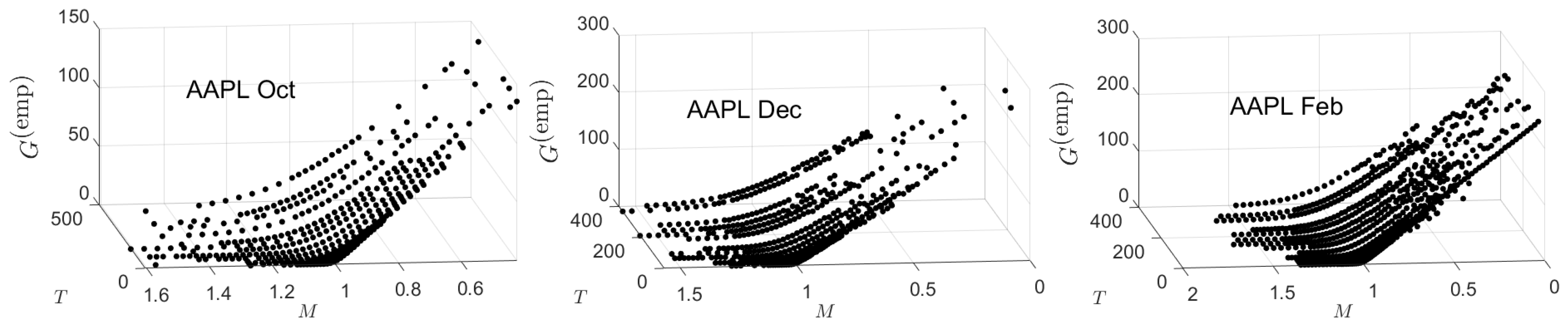
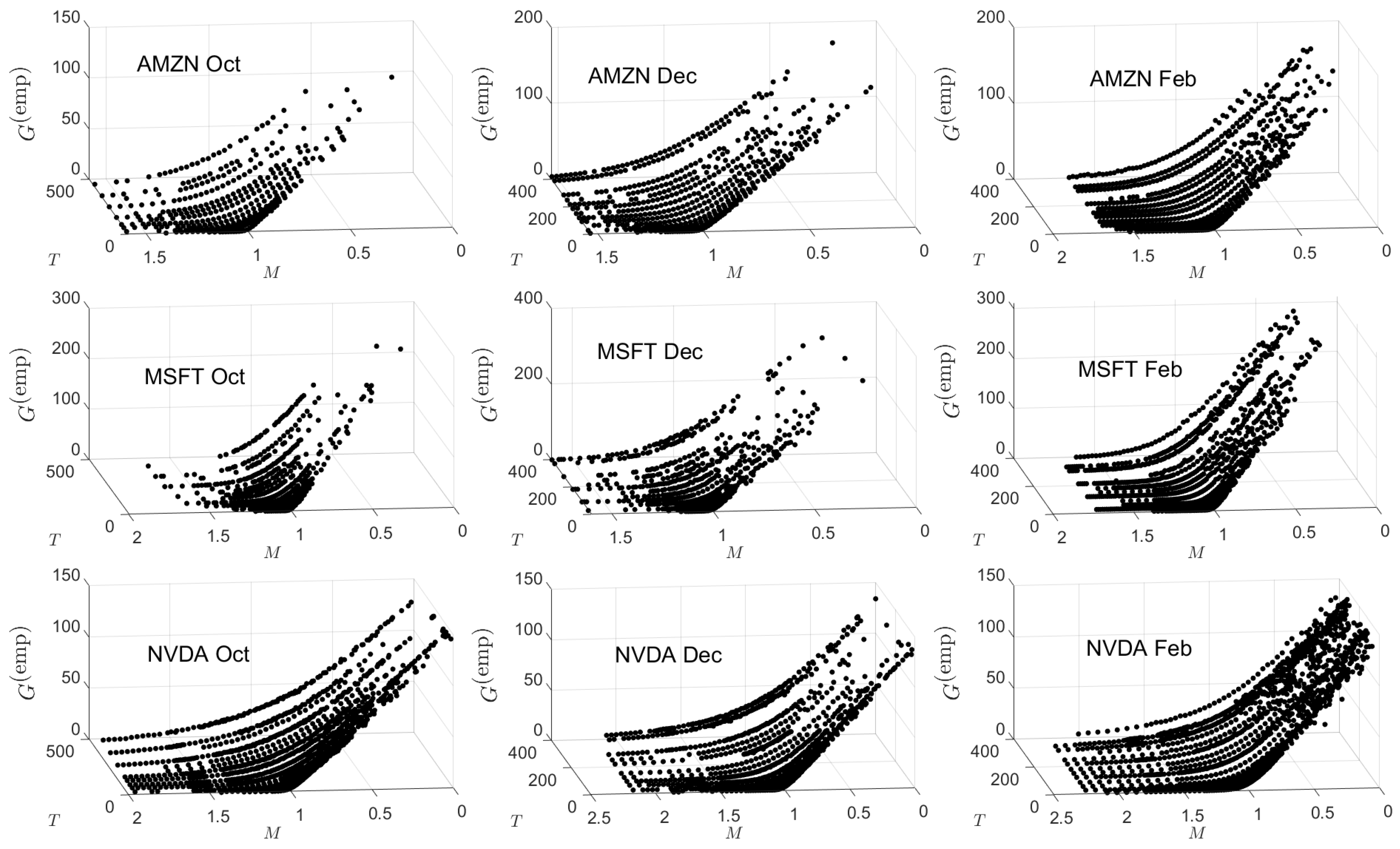
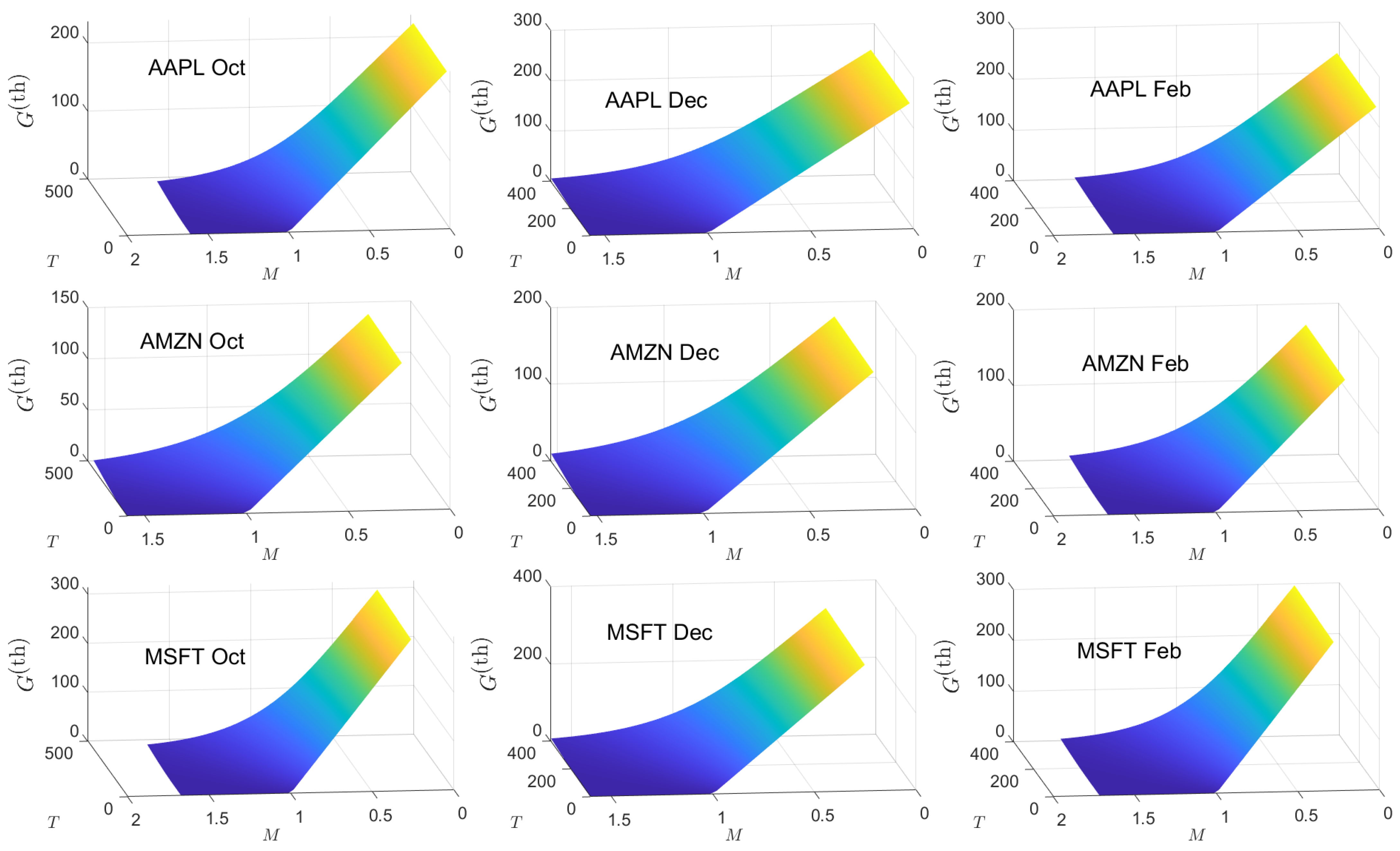
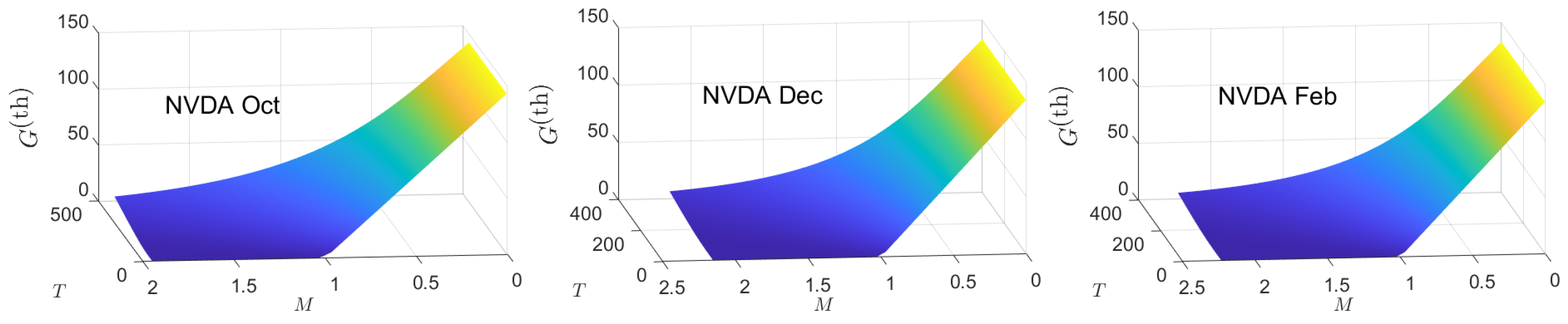
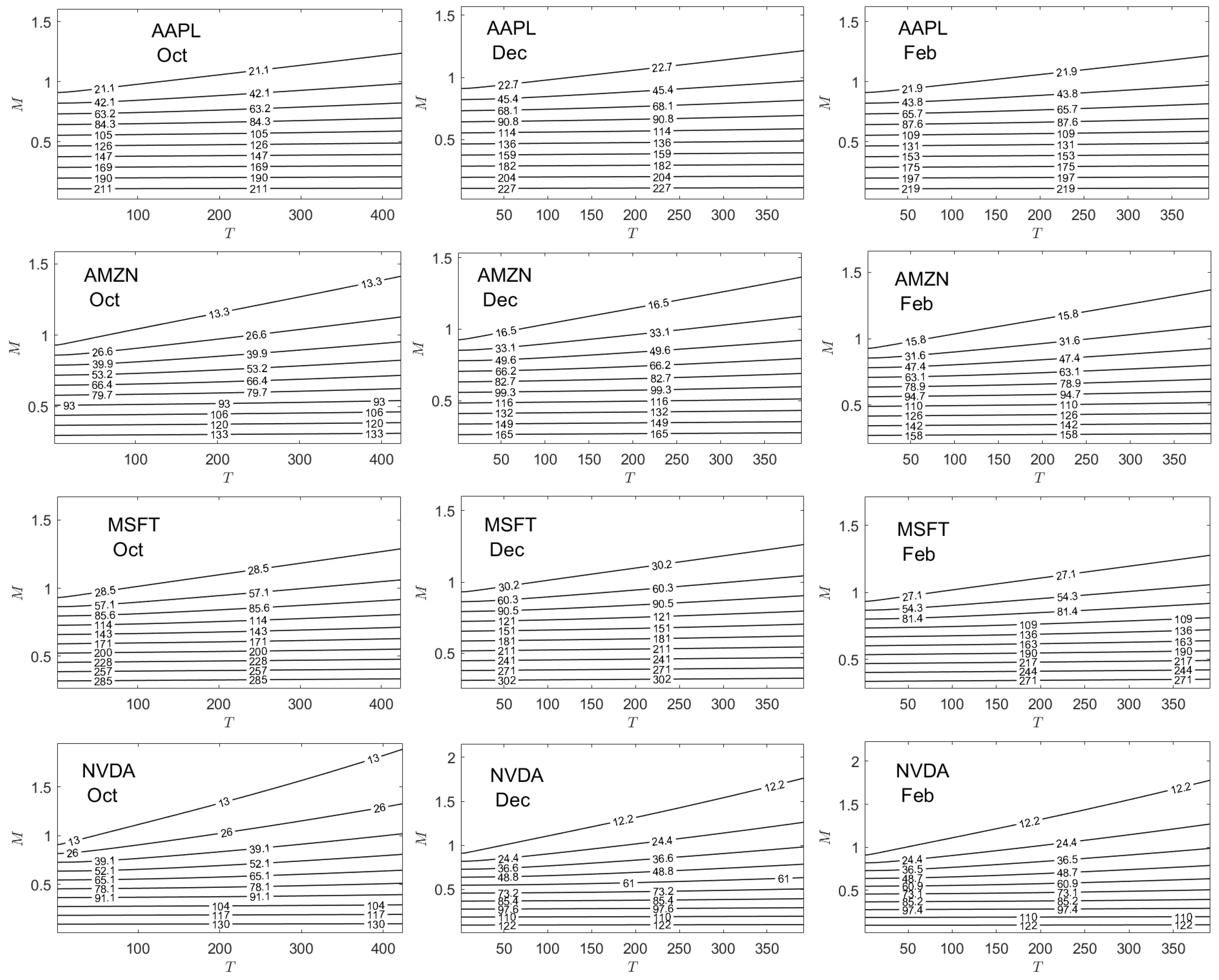
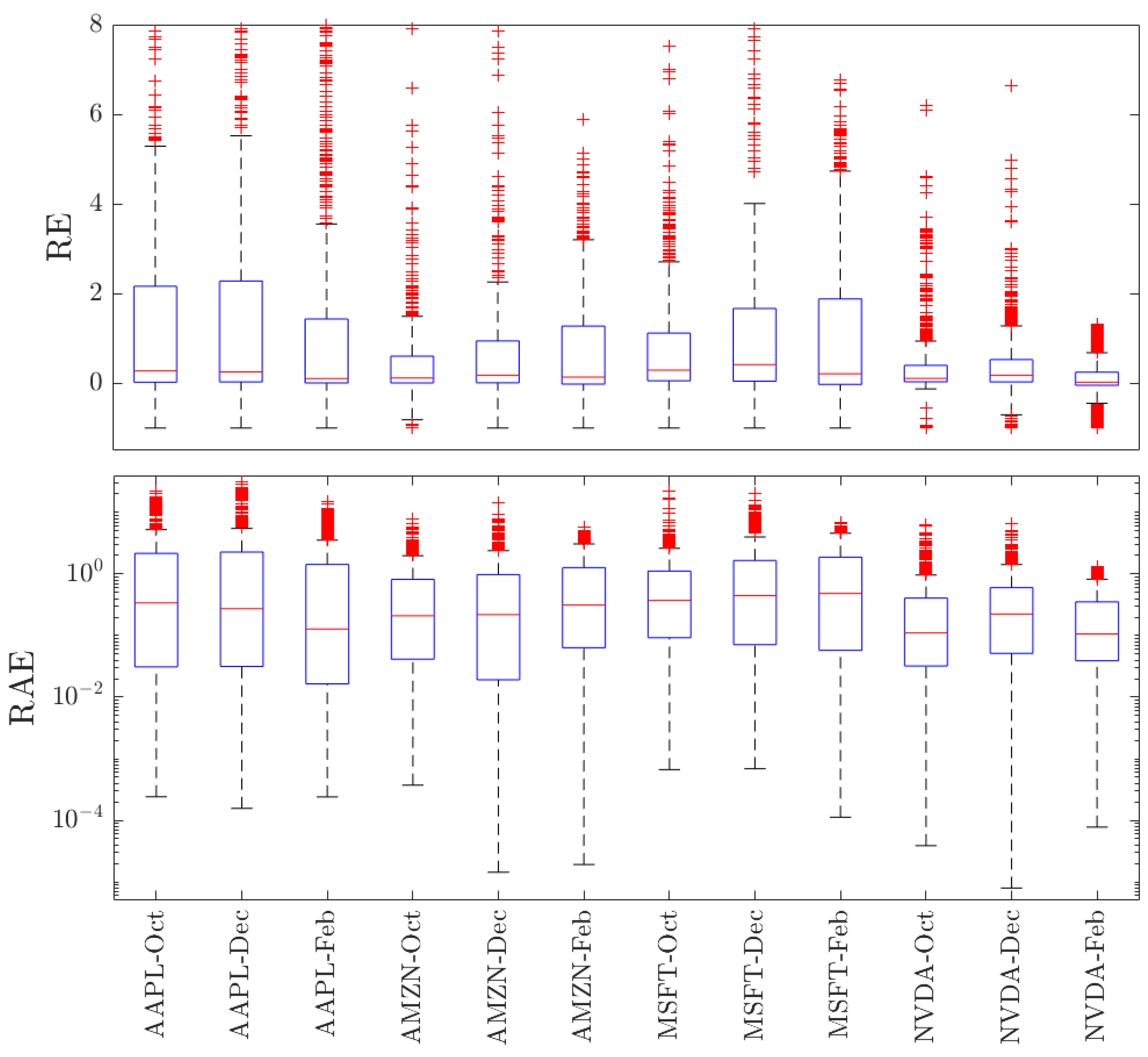
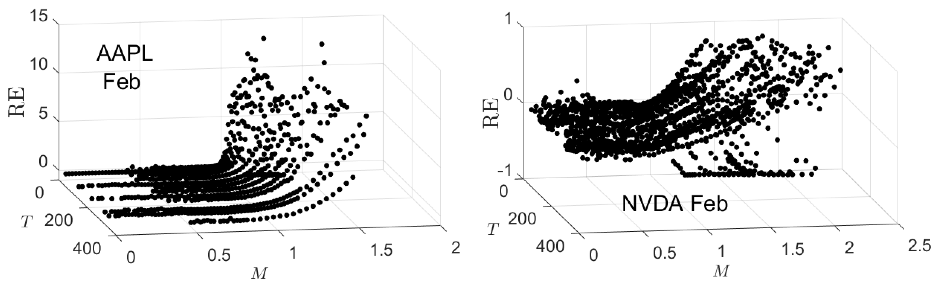
5.1. Option Prices

Let $G^{\left(\mathrm{emp}\right)}(S_0,T_i,K_j)$, $i=1,\dots ,I$, $j=1,\dots ,J$, denote the published prices for a call option having $\mathcal{S}$ as the underlying. Let $G^{\left(\mathrm{th}\right)}\left(S_0,T_i,K_j;{\sigma }_t^{\left(r\right)},{\mu }_t^{\left(r\right)},r_{\mathrm{thr}},r_{f,t}\right)$ denote the respective theoretical option prices computed from the trinomial tree. We computed theoretical call option prices for the maturity times $T=1,2,3,\dots ,T_I$14 and strike prices $K\in \{K_1,\dots ,K_J\}$. The parameters $p_{u,t}$, $p_{m,t}$, $p_{d,t}$, ${\mu }_t^{\left(r\right)}$ and ${\sigma }_t^{\left(r\right)}$ required for the theoretical model were estimated from the historical returns over the relevant eight-year period, as described in Section 4. The subscript t on each parameter refers to the date for which option prices were computed. As each date is known from context, for brevity of notation we drop the t subscript from all parameters in the remainder of Section 5.

Table 1. Parameter values computed from the historical returns.

Stock	${\mathit{S}}_0$	${\mathit{\mu }}^{\left(\mathit{r}\right)}$	${\mathit{\sigma }}^{\left(\mathit{r}\right)}$	${\mathit{p}}_{\mathit{d}}$	${\mathit{p}}_{\mathit{m}}$	${\mathit{p}}_{\mathit{u}}$	${\mathit{r}}_{\mathit{f}}$	Yearly	Daily
		$\times {\mathbf{10}}^{-\mathbf{3}}$	$\times {\mathbf{10}}^{-\mathbf{2}}$		$\times {\mathbf{10}}^{-\mathbf{3}}$			$\times {\mathbf{10}}^{-\mathbf{2}}$	$\times {\mathbf{10}}^{-\mathbf{4}}$
21 October 2024
AAPL	236.48	1.21	1.84	0.461	2.98	0.537	3 Mo	4.73	5.08
AMZN	189.07	0.976	2.08	0.465	1.99	0.533	10 Yr	4.19	1.12
MSFT	418.78	1.12	1.73	0.459	5.47	0.536
NVDA	143.71	2.73	3.25	0.454	3.48	0.543
20 December 2024
AAPL	254.49	1.24	1.84	0.459	2.98	0.538	3 Mo	4.34	4.67
AMZN	224.92	1.09	2.08	0.463	1.99	0.535	10 Yr	4.52	1.21
MSFT	436.60	1.11	1.73	0.456	5.46	0.539
NVDA	134.70	2.46	3.17	0.456	3.48	0.541
21 February 2025
AAPL	245.55	1.15	1.85	0.462	2.49	0.535	3 Mo	4.32	4.65
AMZN	216.58	1.02	2.09	0.467	1.99	0.531	10 Yr	4.42	1.19
MSFT	408.21	1.07	1.75	0.455	4.47	0.540
NVDA	134.43	2.44	3.20	0.456	2.98	0.541

provides the values for the initial price $S_0^{\left(0\right)}\equiv S_0$ and the estimated parameters. Table 1 also provides the US Treasury 10-year and 3-month yield curve rates. (The 3-month rate is used in Section 5.4).

The empirical option prices $G^{\left(\mathrm{emp}\right)}(S_0,T,M)$ are plotted as functions of $T\in \{T_1,\dots ,T_I\}$ and moneyness $M\in \{M_1,\dots ,M_J\}$, $M_j=K_j/S_0$, in Figure A1 (Appendix B). Three-dimensional scatterplots are employed to show how sparsely in T and M the empirical data are populated, as well as to see pricing “irregularities”. The theoretical call option prices $G^{\left(\mathrm{th}\right)}\left(S_0,T,M;{\sigma }^{\left(r\right)},{\mu }^{\left(r\right)},r_{\mathrm{thr}},r_f\right)$, $T\in \{1,2,3,\dots ,T_I\}$, $M\in \{M_1,\dots ,M_J\}$, based on the historical parameter values in Table 1 are plotted as surfaces in Figure A2 (Appendix B). Quantitatively, it is more informative to consider the contours of $G^{\left(\mathrm{th}\right)}(T,M)$. For each surface, 10 evenly spaced contour levels, projected on the $T,M$ plane, are plotted in Figure A3 (Appendix B). From the contours we see, for example, that the at-the-money price $G^{\left(\mathrm{th}\right)}(T,M=1)$ of AMZN computed for 20 December 2024 varies from below $16 at short maturities to approximately $40 at 390 days’ maturity.

As the empirical and theoretical option prices share the common points $(T,M)$, $T\in \{T_1,\dots ,T_I\}$, $M\in \{M_1,\dots ,M_J\}$, we utilized this set of points to investigate theoretical:empirical price differences. Specifically we defined the relative errors

$$\left.\begin{array}{cc}\hfill \mathrm{RE}(T_i,M_j)& ={\displaystyle \frac{G^{\left(\mathrm{th}\right)}(T_i,M_j)}{G^{\left(\mathrm{emp}\right)}(T_i,M_j)}}-1,\hfill \\ \hfill \mathrm{RAE}(T_i,M_j)& =\mathrm{abs}\left(\mathrm{RE}(T_i,M_j)\right),\hfill \end{array}\right\}i=1,\dots ,I,j=1,\dots ,J,$$

(23)

which are computed for all points $(T_i,M_j)$ for which there are empirical data. Figure 2 presents box–whisker summaries of the distributions of RE and RAE values for each combination of stock and option date. The RE distribution indicates that, given the parameter values, the trinomial model predominantly overestimated the option prices. Overall, the trinomial model fitted NVDA option prices the best, AAPL prices the worst. For all 12 stock–date combinations studied, the 75’th percentile for the RAE values did not exceed a value of 2.28; the median RAE value did not exceed 0.484; and the 25’th percentile did not exceed 0.092. The large values of RAE occur out-of-the-money, where empirical option prices are the smallest. In- and at-the-money, the trinomial model produced satisfactory fits. This is illustrated in Figure 3 which plots $\mathrm{RE}(T,M)$ for AAPL and NVDA for 21 February 2025 as a 3D scatterplot. The plots for the other stocks and dates display similar behavior.

Deep out-of-the-money pricing reflects the negative tail behavior of the return distribution. As our pricing model is Gaussian (geometric Brownian motion in the case of constant coefficients), our model is thin-tailed. In reality, asset return distributions are heavy-tailed. We would consequently expect that our model should underestimate deep in- and out-of-the-money option prices. The observation that our theoretical, out-of-the-money option prices are consistently higher than empirical option prices leads us to conclude that option traders were underestimating the out-of-the-money tail risk.

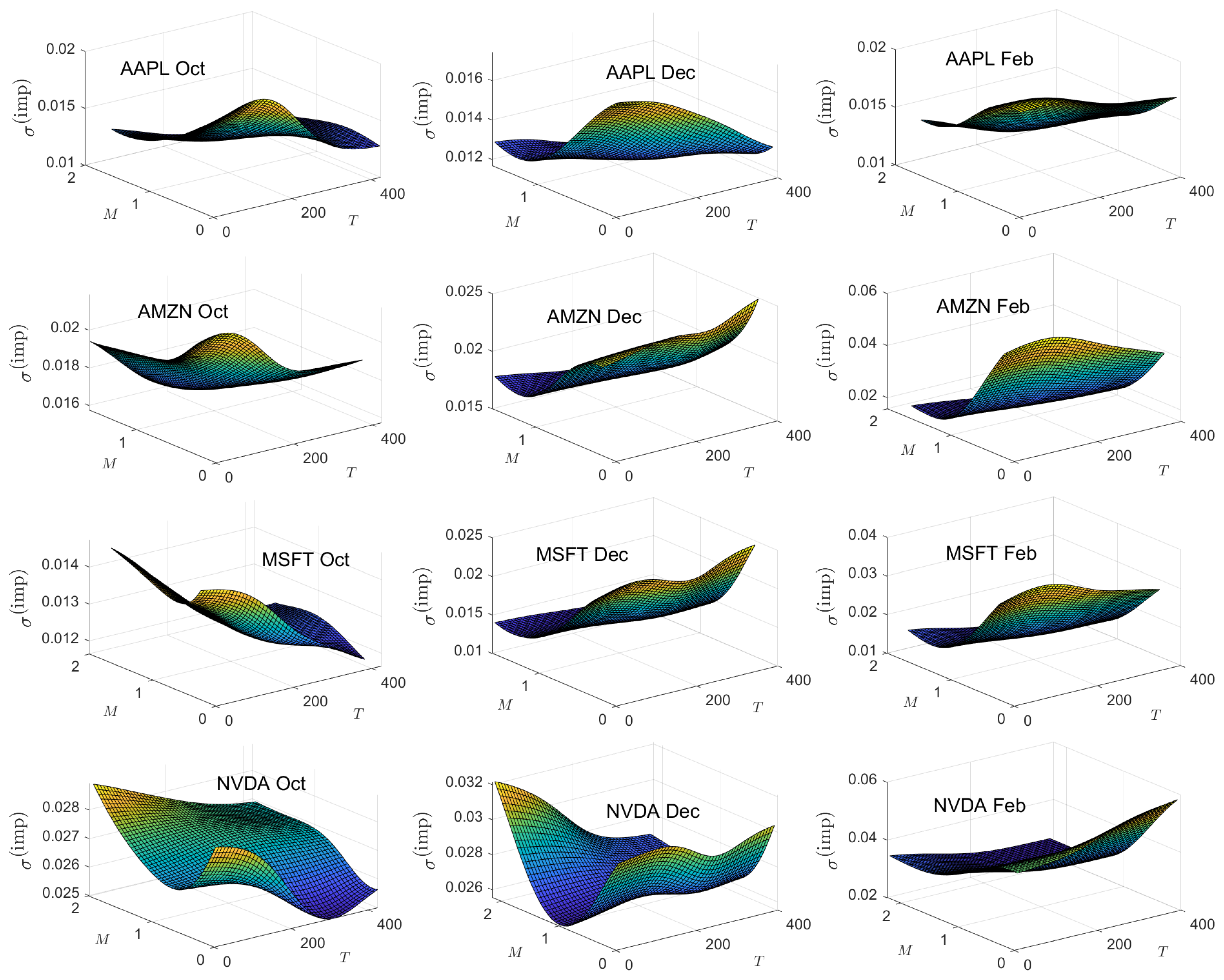
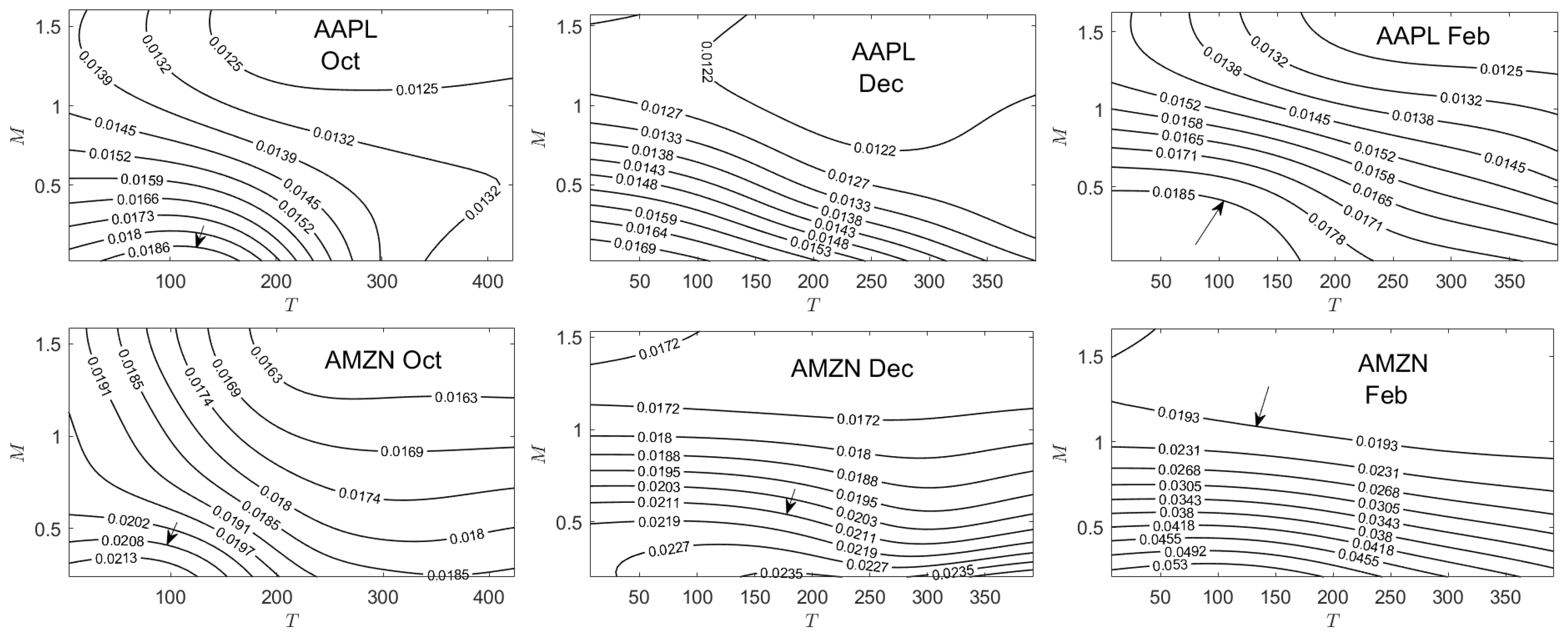
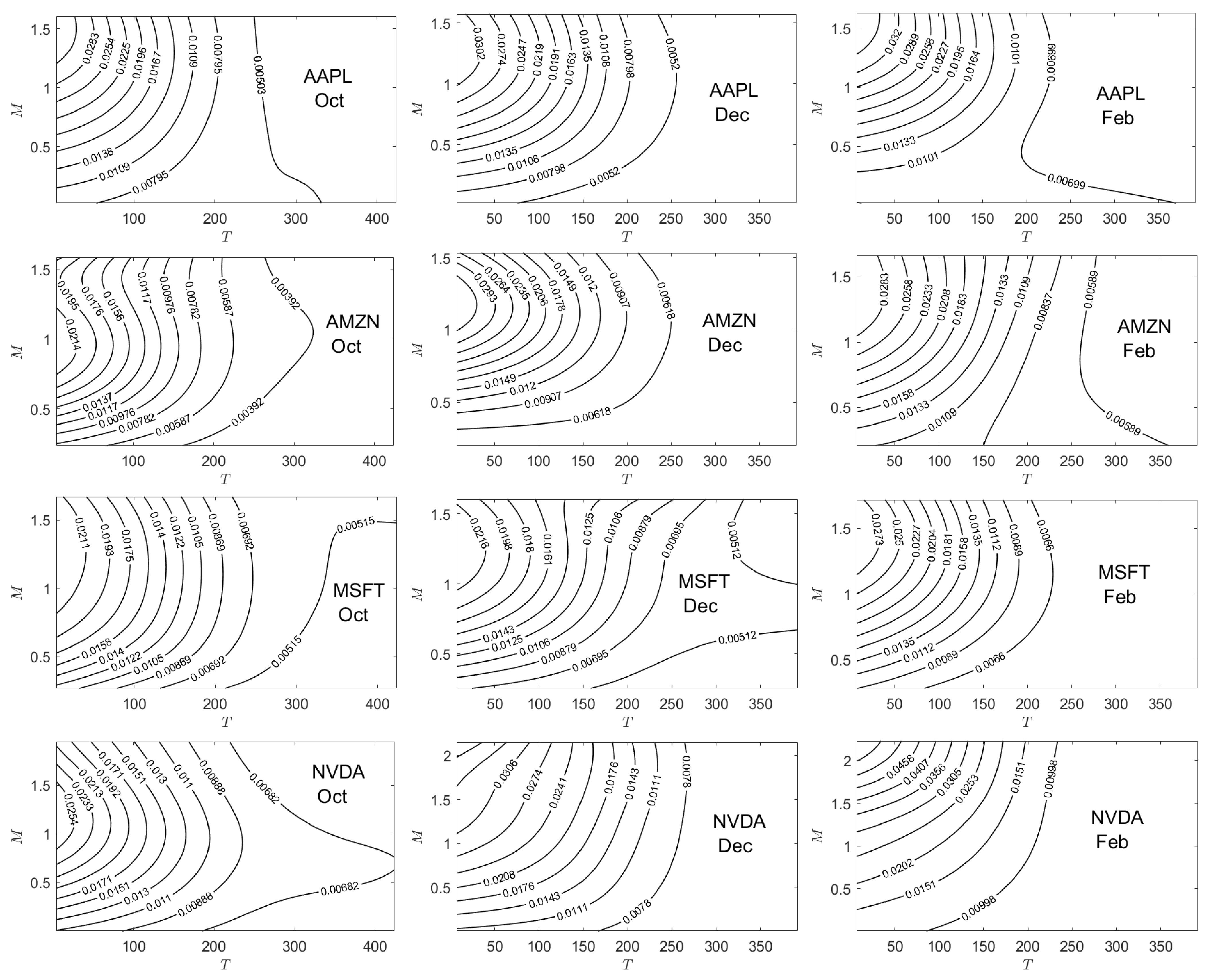
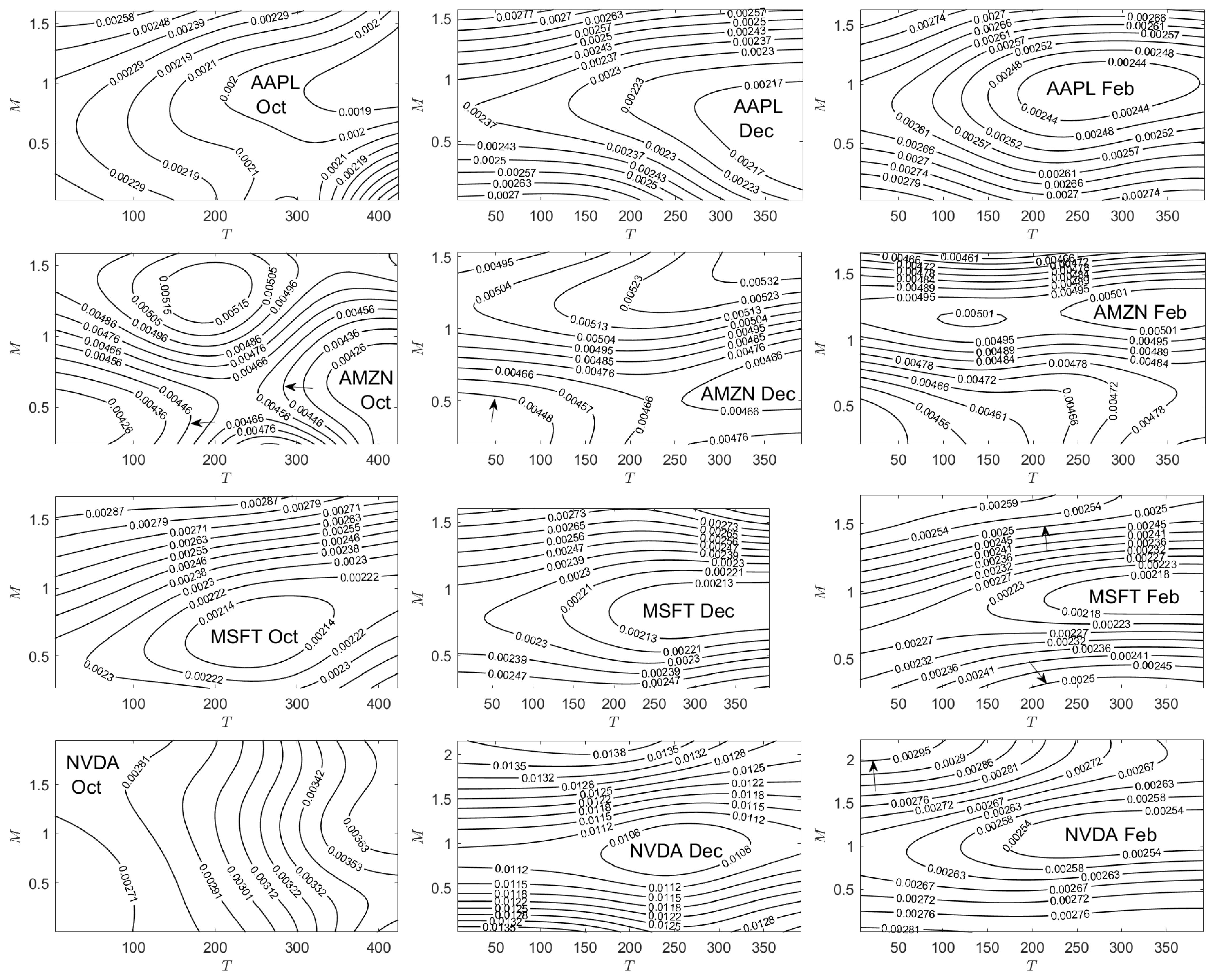
5.2. Implied Volatility

The implied volatility was computed via the optimization

$${\sigma }^{\left(\mathrm{imp}\right)}(T_i,K_j)=\underset{\sigma }{arg\; min}{\left({\displaystyle \frac{G^{\left(\mathrm{th}\right)}\left(S_0,T_i,K_j;\sigma ,{\mu }^{\left(r\right)},r_{\mathrm{thr}},r_f\right)-G^{\left(\mathrm{emp}\right)}(S_0,T_i,K_j)}{G^{\left(\mathrm{emp}\right)}(S_0,T_i,K_j)}}\right)}^2,$$

(24)

for all pairs of values $(T_i,K_j)$ for which there are empirical data. Using a Gaussian kernel smoother, implied volatility values were then computed for all coordinates $(T_i,K_j)$, $i=1,\dots ,I$, $j=1,\dots ,J$.15 The resultant implied volatility surfaces are shown in Figure A4 (Appendix C), while 10 contour levels of ${\sigma }^{\left(\mathrm{imp}\right)}$, projected on the $T,M$ plane, are shown in Figure A5. The implied volatility contour levels generally increase from the out-of-the money region into the in-the-money regions, with smaller dependence on maturity (increasing from the high-maturity-date to the low-maturity-date regions).

Based on the contour levels plotted, one can (approximately) position the contour associated with the appropriate historical value of ${\sigma }^{\left(r\right)}$ listed in Table 1. For example, for AAPL, the closest appropriate contour levels are 0.0186 (Oct) and 0.0185 (Feb). These contours are indicated by arrows. The implied volatility for AAPL in the vast majority of the $(T,M)$ regions falls below that of the historical volatility on these two dates. For AAPL (Dec), all implied volatilities lie below ${\sigma }^{\left(r\right)}$. It is apparent that, for AAPL on these three dates, option traders were anticipating lower future volatilities over the vast majority of the $(T,M)$ region. Similar observations can be deduced for the other three stocks for the three pricing dates.

Another view of the implied volatilities is provided in Figure 4, which uses box–whisker plots to summarize the implied volatility distribution for each stock–date combination. The distribution of implied volatilities is widest on 21 February 2025 and narrowest on 21 October 2024, reflecting the relative uncertainty held by option traders on those dates. From this figure, it is clear that option traders were anticipating lower future volatilities on 21 October 2024 and 20 December 2024. On 21 February 2025, the outlook was less optimistic.

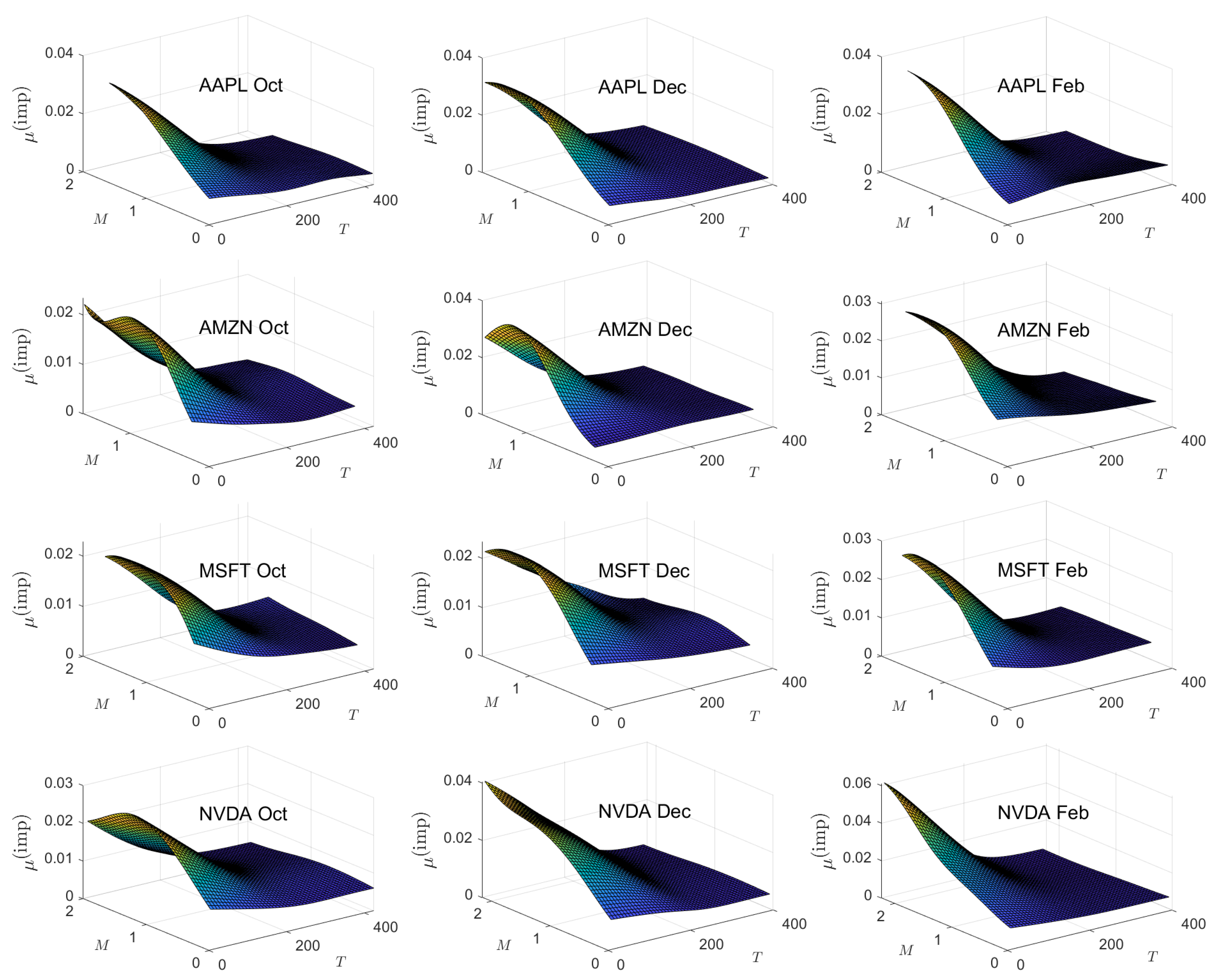
5.3. Implied Mean

The implied mean was computed via the optimization

$${\mu }^{\left(\mathrm{imp}\right)}(T_i,K_j)=\underset{\mu }{arg\; min}{\left({\displaystyle \frac{G^{\left(\mathrm{th}\right)}\left(S_0,T_i,K_j;{\sigma }^{\left(r\right)},\mu ,r_{\mathrm{thr}},r_f\right)-G^{\left(\mathrm{emp}\right)}(S_0,T_i,K_j)}{G^{\left(\mathrm{emp}\right)}(S_0,T_i,K_j)}}\right)}^2.$$

(25)

The resultant implied mean surfaces, and projected contours, are shown in Figure A6 and Figure A7 of Appendix C. The contour levels generally decrease in value as the maturity time T increases, becoming constant at large T. There is a secondary increase in value with moneyness. The box–whisker summaries of the distributions of ${\mu }^{\left(\mathrm{imp}\right)}(T,M)$ are shown in Figure 5. All 12 stock–date distributions are quite similar. In all cases, the entire range of ${\mu }^{\left(\mathrm{imp}\right)}$ values are higher than the respective historical value of ${\mu }^{\left(r\right)}$. For these three dates, option traders appear to be very optimistic regarding projected mean returns for these four stocks.

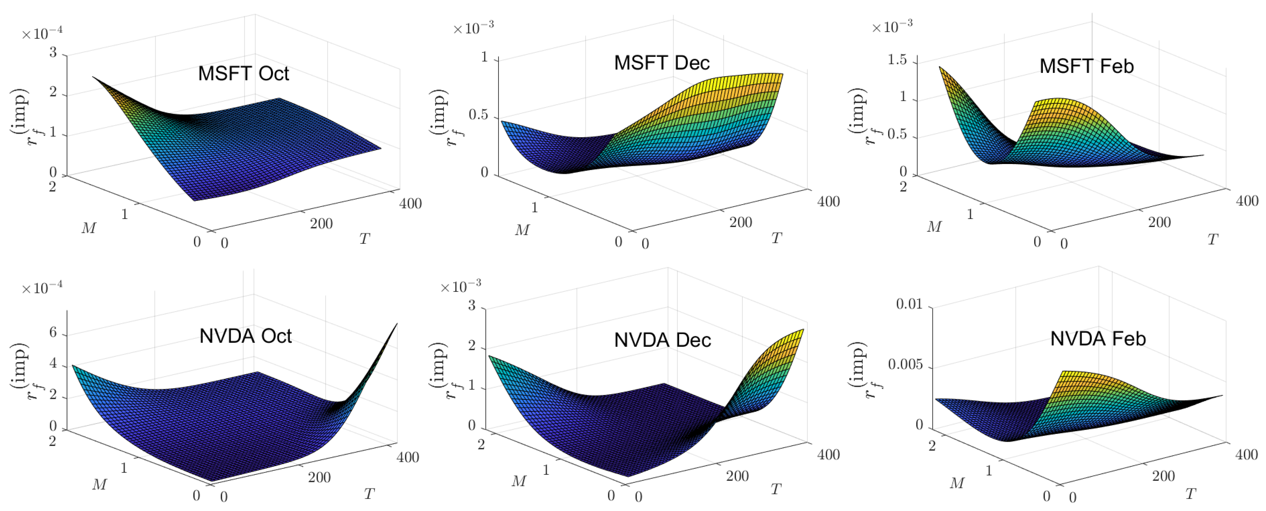
5.4. Implied Risk-Free Rate

The implied risk-free rate was computed via the optimization

$$r_f^{\left(\mathrm{imp}\right)}(T_i,K_j)=\underset{r_f}{arg\; min}{\left({\displaystyle \frac{G^{\left(\mathrm{th}\right)}\left(S_0,T_i,K_j;{\sigma }^{\left(r\right)},{\mu }^{\left(r\right)},r_{\mathrm{thr}},r_f\right)-G^{\left(\mathrm{emp}\right)}(S_0,T_i,K_j)}{G^{\left(\mathrm{emp}\right)}(S_0,T_i,K_j)}}\right)}^2.$$

(26)

Figure 6 presents box–whisker summaries of the distribution of $r_f^{\left(\mathrm{imp}\right)}(T,M)$ values for each stock–date combination. The right-arrows to the left of each box plot indicate the historical value of $r_f$ (3 Mo) and $r_f$ (10 Yr) provided in Table 1. This view makes it easy to see that, for AAPL on 20 December 2024, all values of $r_f^{\left(\mathrm{imp}\right)}(T,M)$ fall below both the $r_f$ (10 Yr) and $r_f$ (3 Mo) values for that date. The implication is that an investor should invest in either US treasury (preferably the 3 Mo as it has the highest yield) rather than this risky stock. In contrast, for NVDA on 21 February 2025, roughly 75% of the $(T,M)$ phase space corresponds to a region where investment in the risky stock is preferable to investment in either treasury.

The resultant implied risk-free rate surfaces and projected contours are shown in Figure A8 and Figure A9 (Appendix C). Select contour levels are provided16 with the contours corresponding to $r_f$ (10 Yr) and $r_f$ (3 Mo) values indicated by arrows. For a given pair of $(T,M)$ values, it is therefore possible to determine whether an investment in the 10 Yr treasury note, the risky asset, or the 3 Mo treasury bill is more appropriate.

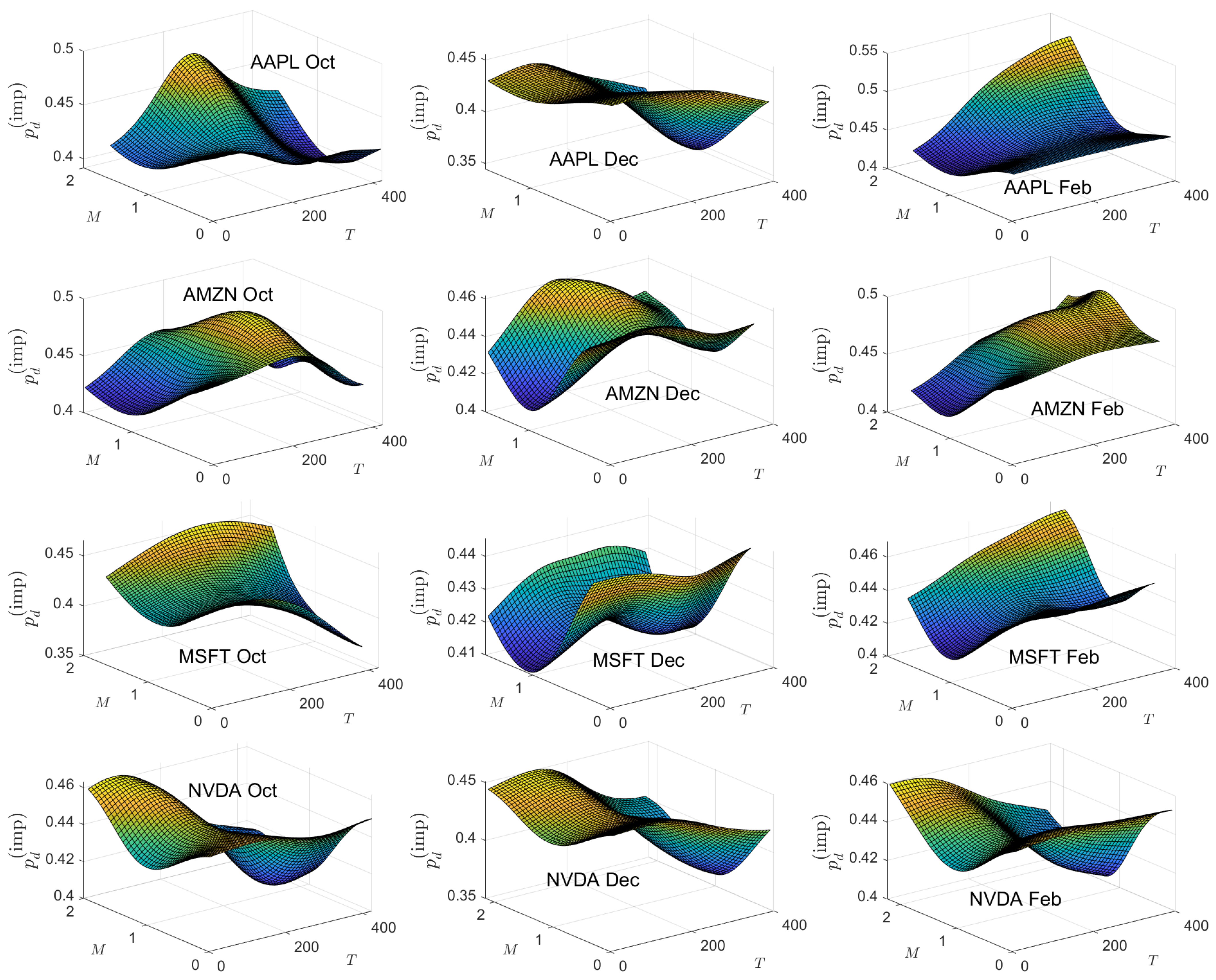
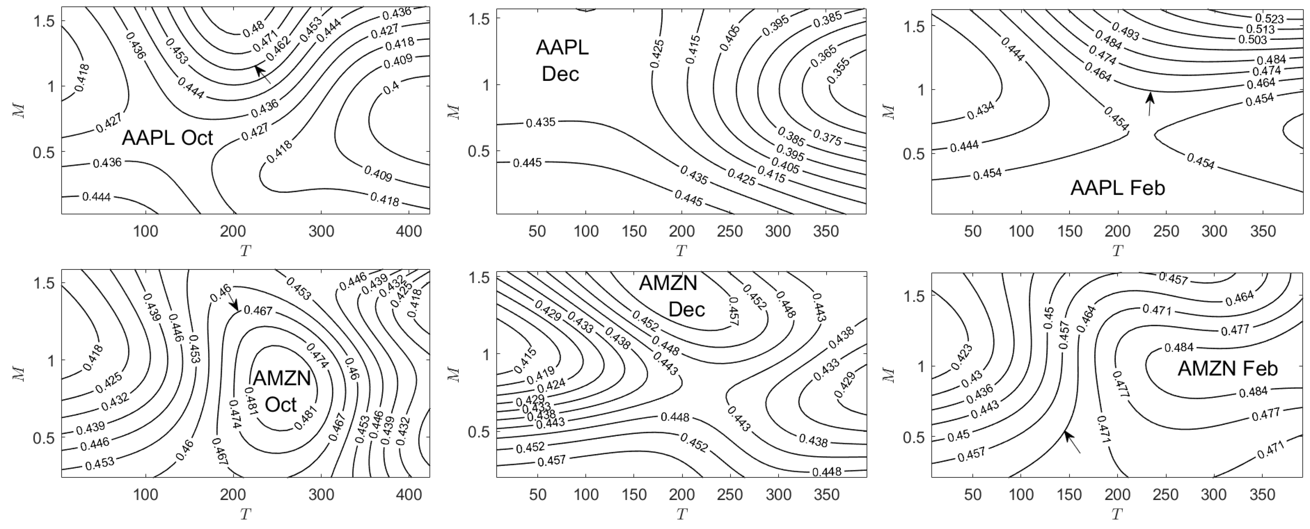
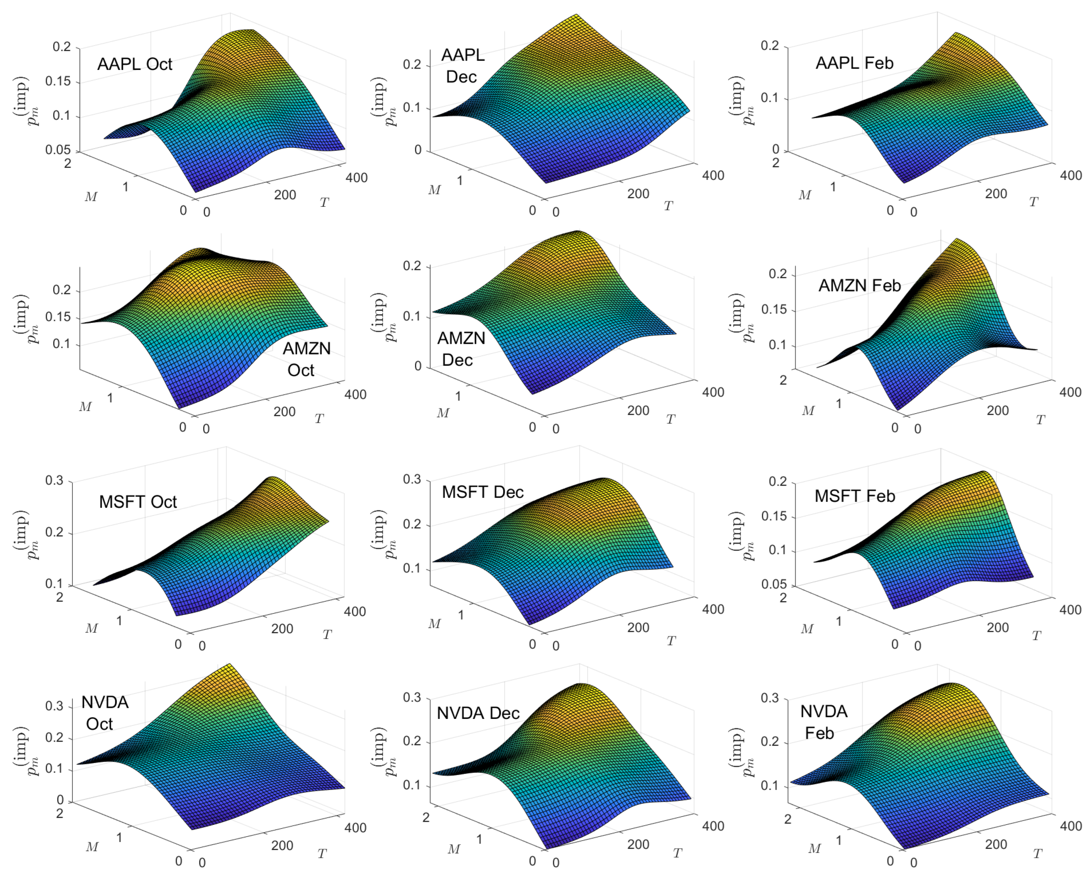
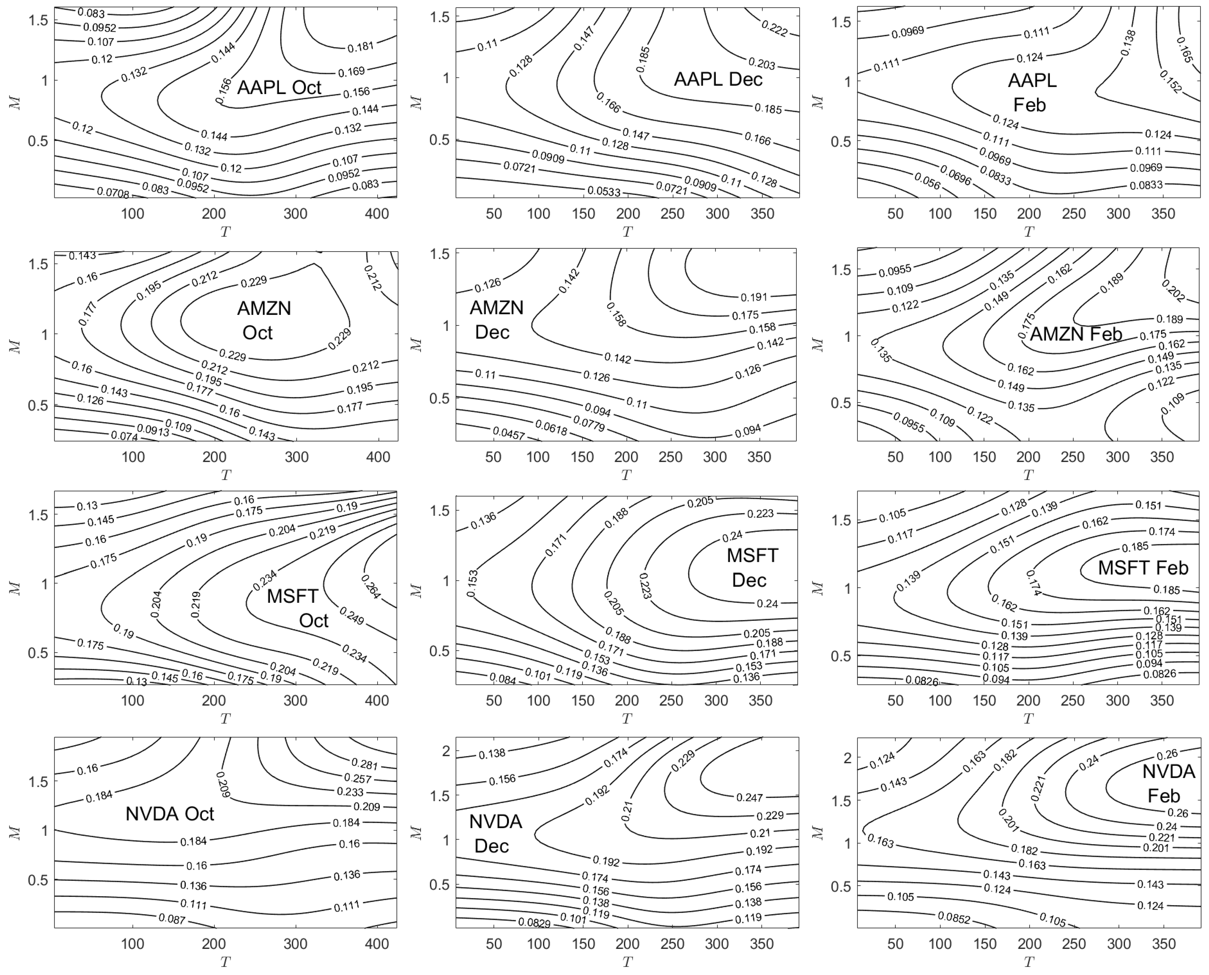
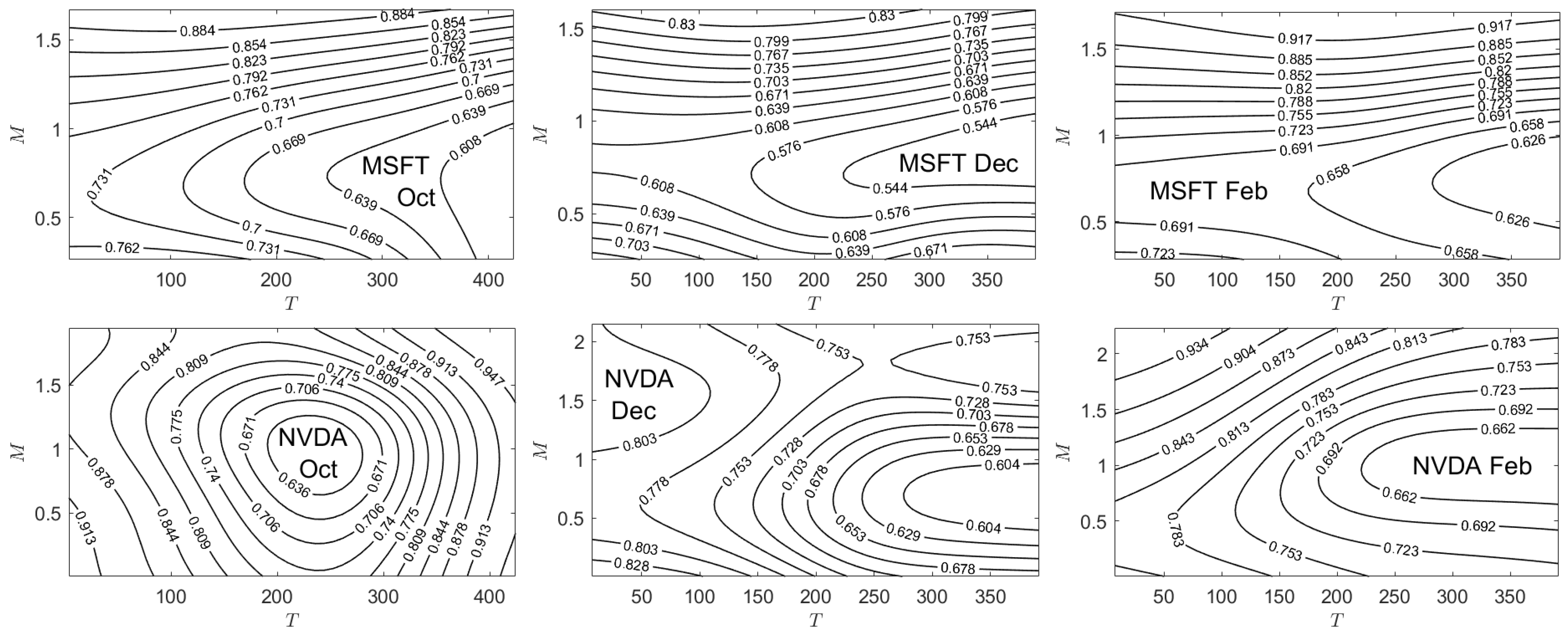
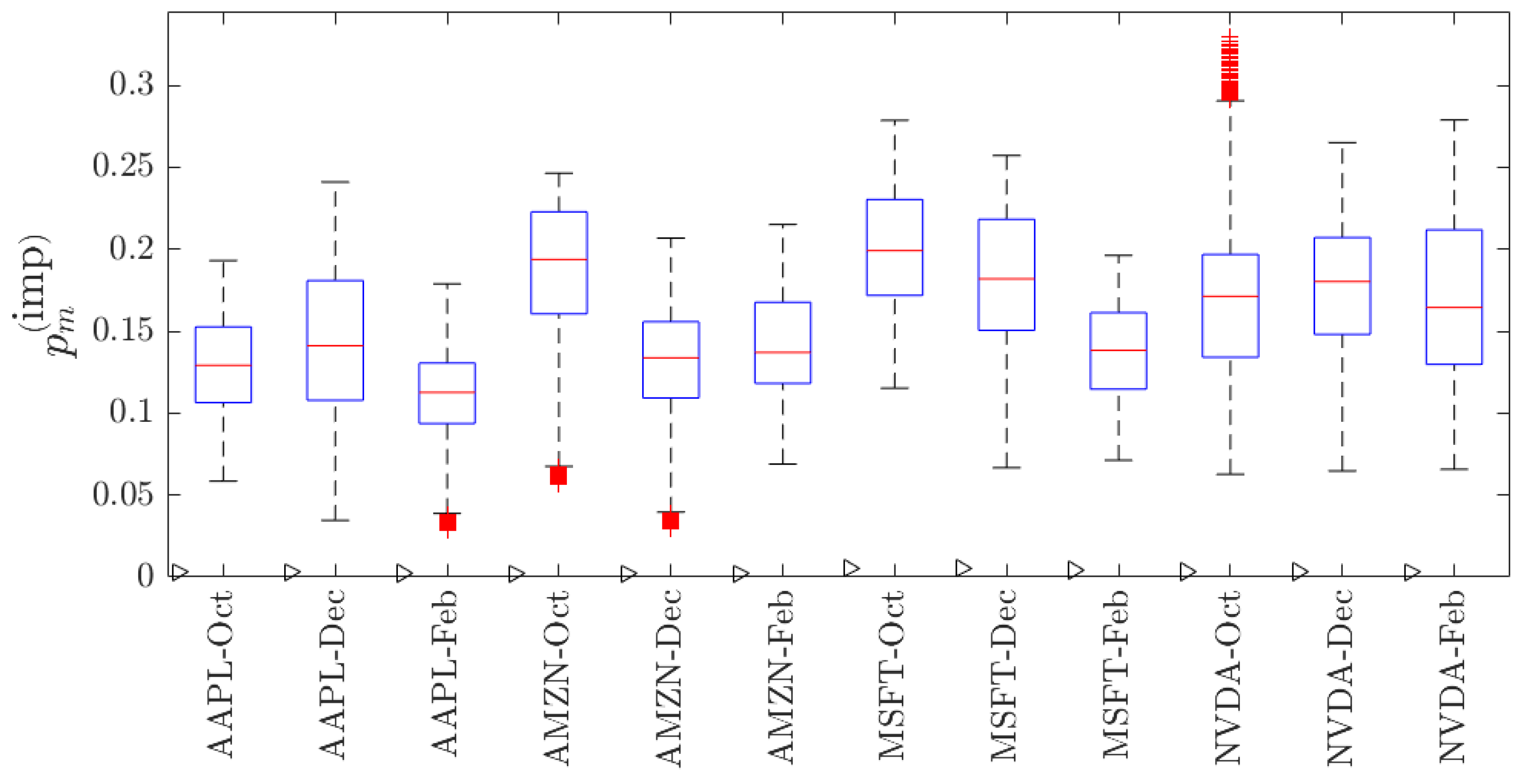
5.5. Implied Price-Change Probability

For the implied parameters ${\sigma }^{\left(r\right)}$, ${\mu }^{\left(r\right)}$ and $r_f$, specification of $r_{\mathrm{thr}}$ completely determines $p_u$, $p_m$ and $p_d$ used on the trinomial tree. However, we now wish to compute implied probabilities for each pair $T_i,K_j$.

5.5.1. Implied $p_d$

As noted in Section 4.2, we consider the computation of implied values for $p_d$ by holding $p_m$ constant (to the appropriate stock value $p_m$ given in Table 1) and requiring $0\le p_d\le 1-p_m$. Thus, the implied probability for $p_d$ was computed via the optimization

$$p_d^{\left(\mathrm{imp}\right)}(T_i,K_j)=\underset{0\le p_d\le 1-p_m}{arg\; min}{\left({\displaystyle \frac{G^{\left(\mathrm{th}\right)}\left(S_0,T_i,K_j;{\sigma }^{\left(r\right)},{\mu }^{\left(r\right)},p_m,p_d,r_f\right)-G^{\left(\mathrm{emp}\right)}(S_0,T_i,K_j)}{G^{\left(\mathrm{emp}\right)}(S_0,T_i,K_j)}}\right)}^2.$$

(27)

Figure 7 presents box–whisker summaries of the distribution of $p_d^{\left(\mathrm{imp}\right)}(T,M)$ values for each stock–date combination. With three exceptions (AAPL-Feb, AMZN-Oct and AMZN-Feb), the $p_d^{\left(\mathrm{imp}\right)}(T,M)$ values fall below the historical value of $p_d$ over the vast majority of the $(T,M)$ region. Thus, for nine of these twelve stock–date combinations, option traders are projecting more favorable probabilities for increasing prices than indicated by the historical value of $p_d$ (for a fixed value of $p_m$, a smaller value of $p_d$ indicates a larger value of $p_u$).

Figure A10 and Figure A11 (Appendix C), respectively, plot the $p_d^{\left(\mathrm{imp}\right)}(T,M)$ surfaces and projected contours for all stock–date combinations. For AAPL-Feb, AMZN-Oct and AMZN-Feb it is interesting to note the difference in location of the $(T,M)$ region for which $p_d^{\left(\mathrm{imp}\right)}(T,M)>p_d$ (that is, the region of $(T,M)$ values where option traders are predicting a greater probability of price reduction than seen historically). For the remaining nine stock–date combinations, when such a region exists, it is generally deep in-the-money.

Using the value $p_m$ and the implied values $p_d^{\left(\mathrm{imp}\right)}(T_i,K_j)$, we computed the values

$$p_u|p_d^{\left(\mathrm{imp}\right)}(T_i,K_j)=1-p_m-p_d^{\left(\mathrm{imp}\right)}(T_i,K_j).$$

(28)

As $p_d^{\left(\mathrm{imp}\right)}(T,M)+p_u|p_d^{\left(\mathrm{imp}\right)}(T,M)=1-p_m$ (a constant), there is no additional information to be gained in plotting $p_u|p_d^{\left(\mathrm{imp}\right)}(T,M)$.17

5.5.2. Implied $p_m$

Implied values for $p_m$ were computed via the optimization

$$p_m^{\left(\mathrm{imp}\right)}(T_i,K_j)=\underset{0\le p_m\le 1-p_d}{arg\; min}{\left({\displaystyle \frac{G^{\left(\mathrm{th}\right)}\left(S_0,T_i,K_j;{\sigma }^{\left(r\right)},{\mu }^{\left(r\right)},p_d,p_m,r_f\right)-G^{\left(\mathrm{emp}\right)}(S_0,T_i,K_j)}{G^{\left(\mathrm{emp}\right)}(S_0,T_i,K_j)}}\right)}^2,$$

(29)

from which we computed the values

$$p_u|p_m^{\left(\mathrm{imp}\right)}(T_i,K_j)=1-p_d-p_m^{\left(\mathrm{imp}\right)}(T_i,K_j).$$

Figure 8 presents box–whisker summaries of the distribution of $p_m^{\left(\mathrm{imp}\right)}(T,M)$ values for each stock–date combination. In each case, the $p_m^{\left(\mathrm{imp}\right)}(T,M)$ values greatly exceed (by, at minimum, multiplicative factors of 5 to 10) the historical value of $p_m$ over the entire $(T,M)$ region; the probability for no significant movement of stock price projected by option traders greatly exceeds the historical value. The larger the value of $p_m^{\left(\mathrm{imp}\right)}(T,M)$, the smaller the probability an option trader places on whether the stock price will go up.18

Figure A12 and Figure A13 (Appendix C), respectively, plot the $p_m^{\left(\mathrm{imp}\right)}(T,M)$ surfaces and contours. At constant maturity T in the short-to-medium time range, the highest value of $p_m^{\left(\mathrm{imp}\right)}$ generally occurs at-the-money ($M=1$). For the longer maturity times, the highest value tends to migrate to larger out-of-the-money values of M. Exceptions are seen for MSFT for which the highest value of $p_m^{\left(\mathrm{imp}\right)}$ stays close to $M=1$. Another exception is AMZN-Oct, where the highest values of $p_m^{\left(\mathrm{imp}\right)}$ are clearly located within the $(T,M)$ region.

As for implied $p_d$, no new information is obtained by examining plots of the values of $p_u|p_m^{\left(\mathrm{imp}\right)}(T,M)$.

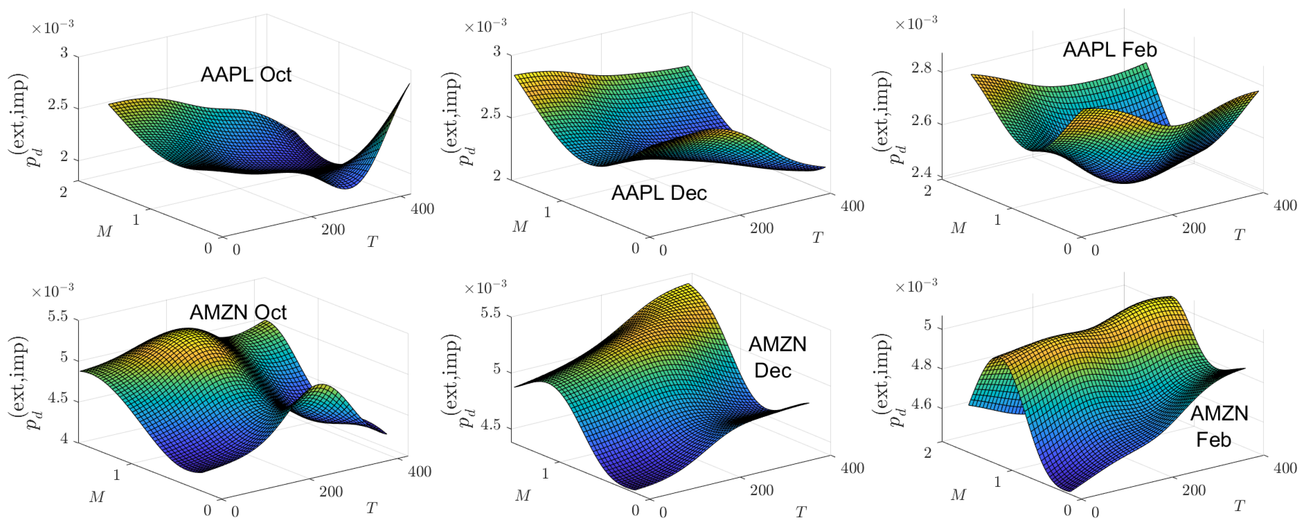
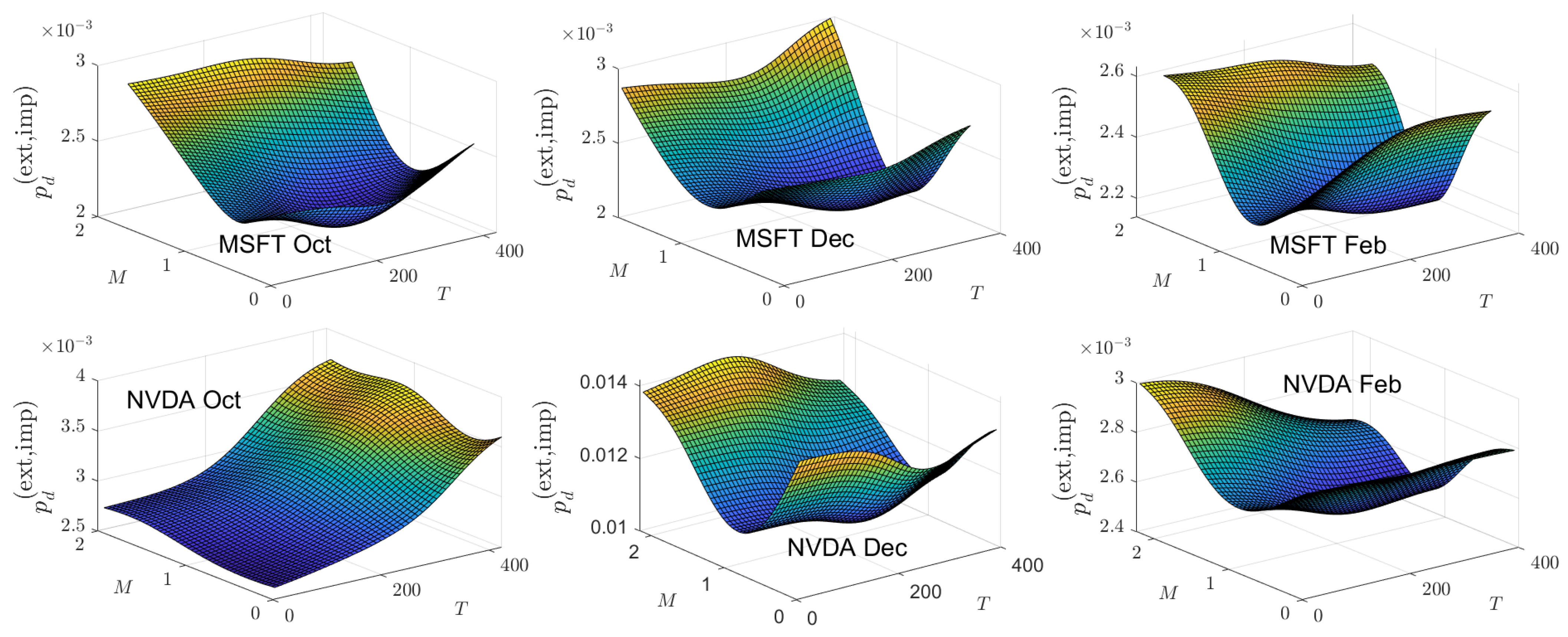
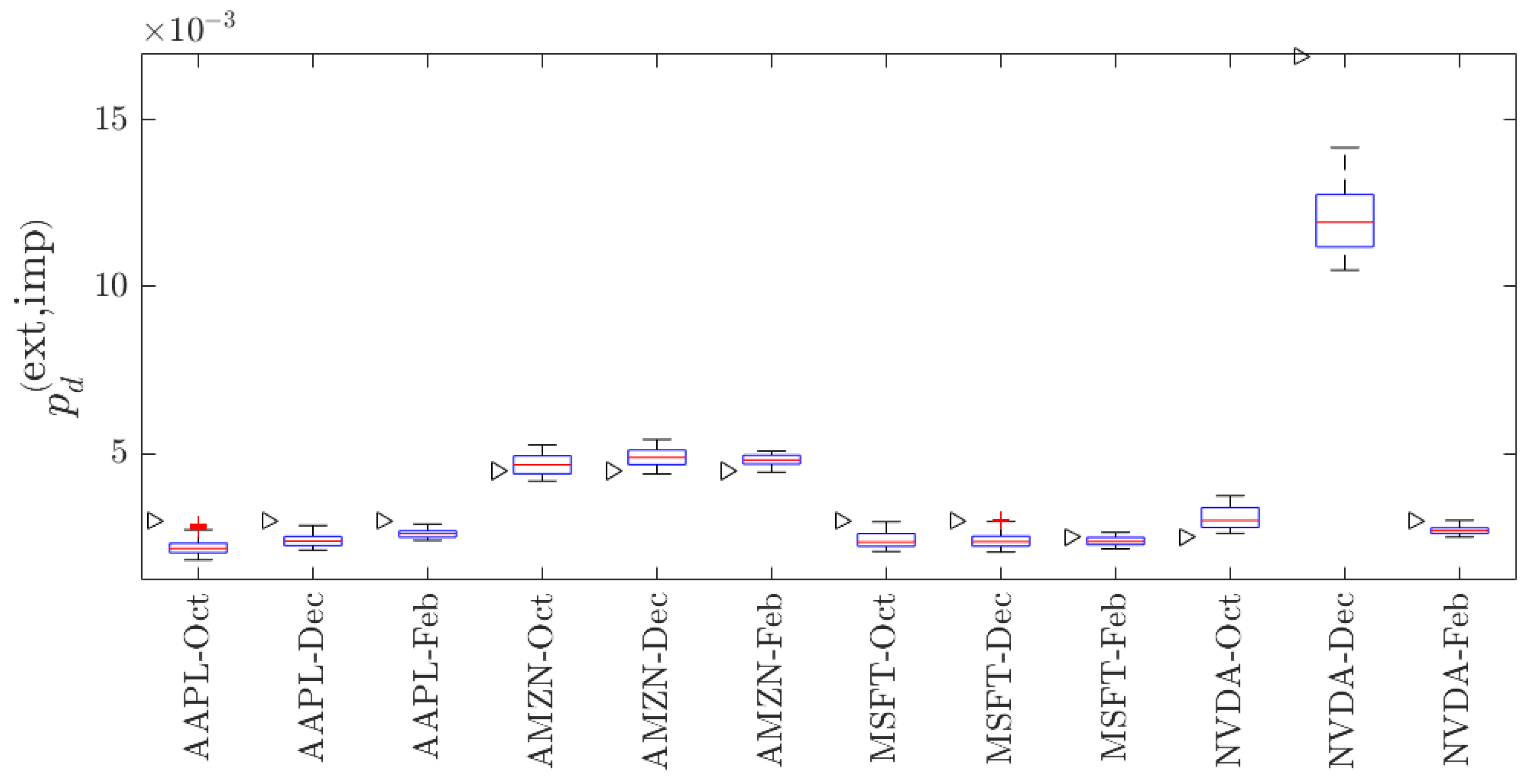
5.6. Implied Extreme Price Change Probabilities

Table 2. Price-change probabilities computed from ${\mathrm{CVaR}}_{0.01}$ and ${\overline{\mathrm{CVaR}}}_{0.01}$.

Stock	${\mathbf{CVaR}}_{0.01}$	${\overline{\mathbf{CVaR}}}_{0.01}$	${\mathit{p}}_{\mathit{d}}^{\left(\mathbf{ext}\right)}$	${\mathit{p}}_{\mathit{m}}^{\left(\mathbf{ext}\right)}$	${\mathit{p}}_{\mathit{u}}^{\left(\mathbf{ext}\right)}$
	$\times {\mathbf{10}}^{-\mathbf{2}}$	$\times {\mathbf{10}}^{-\mathbf{2}}$	$\times {\mathbf{10}}^{-\mathbf{3}}$		$\times {\mathbf{10}}^{-\mathbf{3}}$
21 October 2024
AAPL	−6.69	7.37	2.98	0.9935	3.48
AMZN	−7.28	8.13	4.47	0.9925	2.98
MSFT	−6.09	7.06	2.98	0.9935	3.48
NVDA	−10.4	13.1	2.49	0.9940	3.48
20 December 2024
AAPL	−6.69	7.37	2.98	0.9935	3.48
AMZN	−7.28	8.15	4.47	0.9926	2.98
MSFT	−6.17	7.06	2.98	0.9935	3.48
NVDA *	−6.89	7.44	16.9	0.9697	13.4
21 February 2025
AAPL	−6.69	7.32	2.98	0.9935	3.48
AMZN	−7.28	8.15	4.47	0.9925	2.98
MSFT	−6.26	7.06	2.49	0.9940	3.48
NVDA	−10.8	12.1	2.98	0.9935	3.48

* Values in this row computed using ${\mathrm{CVaR}}_{0.05}$ and ${\overline{\mathrm{CVaR}}}_{0.05}$. See Endnote 19.

lists the historical return values for ${\mathrm{CVaR}}_{0.01}$ and ${\overline{\mathrm{CVaR}}}_{0.01}$, as well as the resultant extreme price-change values $p_d^{\left(\mathrm{ext}\right)}$, $p_m^{\left(\mathrm{ext}\right)}$ and $p_u^{\left(\mathrm{ext}\right)}$.19

5.6.1. Implied $p_d^{\left(\mathrm{ext}\right)}$

Implied values for the extreme probability $p_d^{\left(\mathrm{ext},\mathrm{imp}\right)}$ were computed via the optimization

$$p_d^{\left(\mathrm{ext},\mathrm{imp}\right)}(T_i,K_j)=\underset{0\le p_d\le 1-p_m^{\left(\mathrm{ext}\right)}}{arg\; min}{\left({\displaystyle \frac{G^{\left(\mathrm{th}\right)}\left(S_0,T_i,K_j;{\sigma }^{\left(r\right)},{\mu }^{\left(r\right)},p_m^{\left(\mathrm{ext}\right)},p_d,r_f\right)-G^{\left(\mathrm{emp}\right)}(S_0,T_i,K_j)}{G^{\left(\mathrm{emp}\right)}(S_0,T_i,K_j)}}\right)}^2.$$

(30)

Figure 9 presents box–whisker summaries of the distribution of $p_d^{\left(\mathrm{ext},\mathrm{imp}\right)}(T,M)$ values for each stock–date combination. Generally there is little to no overlap between the historical value $p_d^{\left(\mathrm{ext}\right)}$ and the distribution of $p_d^{\left(\mathrm{ext},\mathrm{imp}\right)}(T,M)$ values, indicating a difference in views between option traders and spot traders. The values of $p_d^{\left(\mathrm{ext},\mathrm{imp}\right)}$ for AMZN are noticeably higher than for the other three stocks, indicating that option traders view the probability of negative returns lower than ${\mathrm{CVaR}}_{0.01}$ to be greater for AMZN. As the $p_d^{\left(\mathrm{ext},\mathrm{imp}\right)}$ values for NVDA-Dec were computed using ${\mathrm{CVaR}}_{0.05}$, its distribution is higher than that of NVDA for the other two dates.

Figure A14 and Figure A15 (Appendix C), respectively, plot the $p_d^{(\mathrm{ext},\mathrm{imp})}(T,M)$ surfaces and their projected contour levels. There is a noticeable variation from stock to stock and date to date in the details of these negative-return-tail-influenced distributions.

5.6.2. Implied $p_m^{\left(\mathrm{ext}\right)}$

Implied values for the extreme probability $p_m^{\left(\mathrm{ext},\mathrm{imp}\right)}$ were computed via the optimization

$$p_m^{\left(\mathrm{ext},\mathrm{imp}\right)}(T_i,K_j)=\underset{0\le p_m\le 1-p_d^{\left(\mathrm{ext}\right)}}{arg\; min}{\left({\displaystyle \frac{G^{\left(\mathrm{th}\right)}\left(S_0,T_i,K_j;{\sigma }^{\left(r\right)},{\mu }^{\left(r\right)},p_m,p_d^{\left(\mathrm{ext}\right)},r_f\right)-G^{\left(\mathrm{emp}\right)}(S_0,T_i,K_j)}{G^{\left(\mathrm{emp}\right)}(S_0,T_i,K_j)}}\right)}^2.$$

(31)

Figure 10 presents box–whisker summaries of the distribution of $p_m^{\left(\mathrm{ext},\mathrm{imp}\right)}(T,M)$ values for each stock–date combination. The historical values $p_m^{\left(\mathrm{ext}\right)}$ are consistently higher than the distribution of $p_m^{\left(\mathrm{ext},\mathrm{imp}\right)}(T,M)$ values; compared to spot traders, option traders are much more optimistic in their view of the probability of extreme positive returns. (Note from (31) that $p_m^{\left(\mathrm{ext},\mathrm{imp}\right)}$ is computed using the fixed value $p_d^{\left(\mathrm{ext}\right)}$. Hence, a smaller value of $p_m^{\left(\mathrm{ext},\mathrm{imp}\right)}$ equates to a larger value of $p_u^{\left(\mathrm{ext},\mathrm{imp}\right)}=1-p_m^{\left(\mathrm{ext},\mathrm{imp}\right)}-p_d^{\left(\mathrm{ext}\right)}$).

For completeness, Figure A16 and Figure A17 (Appendix C), respectively, plot the surface and projected contours of $p_m^{(\mathrm{ext},\mathrm{imp})}(T,M)$. There is relative similarity in the qualitative behavior of these surfaces for AAPL, AMZN, MSFT and NVDA-Feb. The surfaces of NVDA-Oct and NVDA-Dec differ from the rest.

6. Conclusions

This work makes the following significant contributions to the literature on trinomial models.

• We have developed a market-complete trinomial pricing model in which completeness is ensured by a market consisting of a stock and its perpetual derivative as risky assets; a riskless asset (bond); and a European option. The use of the perpetual derivative ensures that the number of Brownian motions driving price stochastics does not increase, thus ensuring the completeness of the market.
• Our model is developed in the natural world and, through the construction of a replicating portfolio, we derive the risk-neutral price dynamics of all four assets. This methodology thus captures the relationship between the risk-neutral and natural-world parameters.
• We derive a new approach for calibrating the probabilities $p_d,p_m$ and $p_d$ for price movements in the natural-world model to empirical data. The approach is based upon hypothesis testing on sub-sample mean values.
• As a result of capturing the explicit relationship between the risk-neutral and natural-world parameters, using call option data from four of the “Magnificent Seven” technology stocks, we compute implied surfaces for all parameters in the model. Examination of the contour levels of an implied parameter surface may split the surface into two regimes —“above and below” the historical value for that parameter—allowing for a comparison of the views of option and spot traders relative to the future performance of that parameter.

References

- Ahn, J., & Song, M. (2007). Convergence of the trinomial tree method for pricing European/American options. Applied Mathematics and Computation, 189(1), 575–582. [Google Scholar]
- Bates, D. S. (1996). Jumps and stochastic volatility: Exchange rate processes implicit in Deutsche Mark options. Review of Financial Studies, 9, 69–108. [Google Scholar] [CrossRef]
- Black, F., & Scholes, M. (1973). The pricing of options and corporate liabilities. Journal of Political Economy, 81(3), 637–654. [Google Scholar]
- Boyle, P. P. (1986). Option valuation using a tree-jump process. International Options Journal, 3, 7–12. [Google Scholar]
- Boyle, P. P. (1988). A lattice framework for option pricing with two state variables. Journal of Financial and Quantitative Analysis, 23(1), 1–12. [Google Scholar]
- Boyle, P. P., Evnine, J., & Gibbs, S. (1989). Numerical evaluation of multivariate contingent claims. Review of Financial Studies, 2, 241–251. [Google Scholar]
- Boyle, P. P., & Lau, S. H. (1994). Bumping up against the barrier with the binomial method. Journal of Derivatives, 1, 6–14. [Google Scholar]
- Chan, J. H., Joshi, M., Tang, R., & Yang, C. (2009). Trinomial or binomial: Accelerating American put option price on trees. Journal of Futures Markets, 29(9), 797–893. [Google Scholar]
- Cox, J. C., Ross, S. A., & Rubinstein, M. (1979). Option pricing: A simplified approach. Journal of Financial Economics, 7(3), 229–263. [Google Scholar]
- Davydov, Y., & Rotar, V. (2008). On a non-classical invariance principle. Statistics & Probability Letters, 78, 2031–2038. [Google Scholar]
- Deutsch, H.-P. (2009). Derivatives and internal models (4th ed.). Palgrave Macmillan. [Google Scholar]
- Florescu, I., & Viens, F. (2008). Stochastic volatility: Option pricing using a multinomial recombining tree. Applied Mathematical Finance, 15, 151–181. [Google Scholar]
- Hilliard, J. E., & Schwartz, A. (1996). Binomial option pricing under stochastic volatility and correlated state variables. Journal of Derivatives, 4(1), 23–39. [Google Scholar]
- Hu, Y., Shirvani, A., Lindquist, W. B., Fabozzi, F. J., & Rachev, S. T. (2020). Option pricing incorporating factor dynamics in complete markets. Journal of Risk and Financial Management, 13(12), 321. [Google Scholar]
- Jarrow, R., & Rudd, A. (1983). Option pricing. Dow Jones-Irwin. [Google Scholar]
- Josheski, D., & Apostolov, M. (2020). A review of the binomial and trinomial models for option pricing and their convergence to the Black-Scholes model determined option prices. Econometrics, 24(2), 53–85. [Google Scholar] [CrossRef]
- Kamrad, B., & Ritchen, P. (1991). Multinomial approximating models for options with k state variables. Management Science, 37, 1640–1652. [Google Scholar]
- Kim, Y. S., Stoyanov, S. V., Rachev, S. T., & Fabozzi, F. J. (2019). Enhancing binomial and trinomial equity option pricing models. Finance Research Letters, 28, 185–190. [Google Scholar]
- Langat, K. K., Mwaniki, J. I., & Kiprop, G. K. (2019). Pricing options using trinomial lattice method. Journal of Finance and Economics, 7, 81–87. [Google Scholar]
- Leisen, D. P. J., & Reimer, M. (1996). Binomial models for option valuation—Examining and improving convergence. Applied Mathematical Finance, 3(4), 319–346. [Google Scholar]
- Lilyana, D., Subartini, B., Riaman, R., & Supriatna, A. K. (2021). Calculation of call option using trinomial tree method and Black-Scholes method: Case study of Microsoft Corporation. Journal of Physics: Conference Series, 1722, 012064. [Google Scholar]
- Lindquist, W. B., & Rachev, S. T. (2025). Alternatives to classical option pricing. Annals of Operations Research, 346, 489–509. [Google Scholar]
- Ma, J., & Zhu, T. (2015). Convergence rates of trinomial tree methods for option pricing under regime-switching models. Applied Mathematics Letters, 39, 13–18. [Google Scholar]
- Madan, D. B., Milne, F., & Shefrin, H. (1989). The multinomial option pricing model and its Brownian and Poisson limits. Review of Financial Studies, 2, 251–265. [Google Scholar]
- Merton, R. C. (1973). Theory of rational option pricing. The Bell Journal of Economics and Management Science, 4(1), 141–183. [Google Scholar]
- Rubinstein, M. (1998). Edgeworth binomial trees. The Journal of Derivatives, 5(3), 20–27. [Google Scholar]
- Sharpe, W. F. (1978). Investments. Prentice-Hall. [Google Scholar]
- Shirvani, A., Stoyanov, S. V., Rachev, S. T., & Fabozzi, F. J. (2020). A new set of financial instruments. Frontiers in Applied Mathematics and Statistics, 6, 606812. [Google Scholar]
- Skorokhod, A. V. (2005). Basic principles and applications of probability theory. Springer. [Google Scholar]
- Tian, Y. (1993). A modified lattice approach to option pricing. The Journal of Futures Markets (1986–1998), 13, 563–577. [Google Scholar]
- Yuen, F. L., & Yang, H. (2010). Option pricing with regime switching by trinomial tree method. Journal of Computational and Applied Mathematics, 233(8), 1821–1833. [Google Scholar]