Optimizing Portfolios with Pakistan-Exposed Exchange-Traded Funds: Risk and Performance Insight

Abstract

This study examines the investment landscape of Pakistan as an emerging and frontier market, focusing on implications for international investors, particularly those in the United States, through exchange-traded funds (ETFs) with exposure to Pakistan. The analysis encompasses 30 ETFs with varying degrees of exposure to Pakistan, covering the period from 1 January 2016 to February 2024. This research highlights the potential benefits and risks associated with investing in these ETFs, emphasizing the importance of thorough risk assessments and portfolio performance comparisons. By providing descriptive statistics and performance metrics based on historical optimization, this paper aims to equip investors with the necessary insights to make informed decisions when optimizing their portfolios with Pakistan-exposed ETFs. The second part of the paper introduces and assesses dynamic optimization methodologies. This section is designed to explore the adaptability and performance metrics of dynamic optimization techniques in comparison with conventional historical optimization methods. By integrating dynamic optimization into the investigation, this research aims to offer insights into the efficacy of these contrasting methodologies in the context of Pakistan-exposed ETFs. The findings underscore the significance of Pakistan’s market dynamics within the broader context of emerging markets, offering a pathway for diversification and potential growth in investment strategies.

1. Introduction

Pakistan has been categorized in the realm of emerging and frontier markets. The analysis of exchange-traded funds (ETFs) with exposure to Pakistan offers a unique perspective on emerging and frontier market investments in terms of portfolio diversification for international investors, given the changing macroeconomic environment and market dynamics. International investors can take on exposure to Pakistan by using brokerage accounts to purchase scrips directly from the stock market, or they can diversify their portfolios by investing in emerging-market ETFs with exposure to Pakistan. For instance, the Global X MSCI Pakistan ETF (PAK) that was created and managed by Global X Management Company LLC was an ETF that tracked the diverse range of Pakistani firms across sectors like the financial, energy, telecommunication and consumer goods sectors and provided exposure to Pakistan’s stock market. This was indeed the first US-listed ETF specifically focused on the Pakistani stock market.

Emerging markets are ahead of frontier markets in terms of economic growth, market size, liquidity and having a robust regulatory environment. For instance, the countries in BRICS (Brazil, Russia, India, China and South Africa) are classified as emerging markets. In contrast, countries like Bangladesh, Sri Lanka, Qatar, Oman, etc., are classified in the frontier markets category. Although there is the potential for substantial growth in these markets for investors, frontier markets are considered to be in the high-risk category due to their less developed financial markets and higher volatility.

Pakistan’s market status was upgraded from frontier to emerging back in November 2016 by MSCI, but it was downgraded to frontier status in November 2021 due to a reduction in the market size and the illiquidity of the stock market. PAK was launched on 23 April 2015; however, it was delisted on 16 February 2024. The delisting has been attributed to various factors, including political and economic uncertainty, low trading volumes, limited market depth, the low liquidity of the assets under management and varying investors’ impressions with respect to Pakistan’s market classification wavering between the emerging and frontier categories. The key indicators of Pakistan’s stock market for the last five years are given in

Table 1. Pakistan Stock Exchange Summary of Key Indicators (2020–2024). Source: Pakistan Stock Exchange.

Variable	2020	2021	2022	2023	2024
Total No. of Listed Companies	531	533	531	524	524
Total Listed Capital (Rs. in Millions)	1,421,094	1,485,103	1,552,728	1,665,477	1,694,457
Total Market Capitalization (Rs. in Millions)	8,035,364	7,684,637	6,500,828	9,062,903	10,169,955
KSE-100™ Index	43,755	44,596	42,420	60,451	75,878
KSE-30™ Index	18,180	17,502	14,836	20,777	24,343
KMI-30 Index	71,168	71,687	68,278	104,729	125,780
KSE All Share Index	30,780	30,727	27,533	41,916	48,828
PSX-KMI All Shares Index	21,718	22,027	19,987	30,664	34,824
New Companies Listed During the Year	3	7	2	1	6
Listed Capital of New Companies (Rs. in Millions)	14,197	16,009	2644	3,932	79,953
New Debt Instruments Listed During the Year	7	5	0	5	3
Listed Capital of New Debt Instruments (Rs. in Millions)	246,967	25,100	0	31,200	6,075
Average Daily Turnover—Regular Market (Shares in Mn, YTD)	330	474	230	323	450
Average Value of Daily Turnover—Regular Market (Rs in Mn, YTD)	12,271	16,935	6,950	10,076	16,797
Average Daily Turnover—Future Market (Shares in Mn, YTD)	102	141	94	106	168
Average Value of Daily Turnover—Future Market (Rs. in Mn, YTD)	4740	8315	3574	4388	6764

, and the returns of different asset classes in 2023 are given in

Table 2. Pakistan Asset Returns in 2023. Source: Topline Securities.

Category	Explanation	PKR Return
KSE-100	Total Return with Dividend	53%
Naya Pakistan US$ Certificate	Including 6.5% Return	33%
Commercial Plots Price Index—Karachi	Source: Zameen.com *	29%
US$	Interbank Market Rate	25%
T-Bill	Reinvest after 3 Months	23%
Gold	Source: Karachi Saraf	18%
House Price Index—Karachi	Source: Zameen.com *	18%
Bank Saving Deposit	Avg. Bank Rate from SBP	17%
PIBs (3-Year Bond)	With Coupon	13%
Special Saving Certificate (SSC)	First-Year Return	13%
Naya Pakistan PKR Certificate	Investment at Beginning of 2023	11%
Residential Plots Price Index—Karachi	Source: Zameen.com *	6%

* Data sourced from Zameen.com, accessed on 15 December 2024.

.

According to Woetzel et al. (2018) and OECD (2019), Asian emerging markets have experienced some of the most robust economic growth rates and outstanding returns in the past, presenting Asia as the world’s leading emerging market region. Among these markets, Pakistan has become more prominent. Bloomberg ranked the Pakistan Stock Exchange (PSX) in the top 10 best-performing stock markets in the world for three straight years from 2012 to 2014. Stock markets previously considered as outcasts in the emerging markets world have been among the world’s best-performing stock markets during 2024, and Pakistan is one of them, as the market has risen 30% since its inception in 2024, leaving behind the markets of Taiwan and India (Jilani, 2024).

Despite various structural problems, Pakistan’s market can still be a good potential avenue for investment for US investors looking for portfolio diversification. Pakistan’s economic sector, driven by sectors like textiles, agriculture and the growing IT industry, provides unique exposure. One of the most important aspects of this market is its relatively low correlation with the US and European markets. Berger et al. (2011) studied frontier market equities, including Pakistan, and found that these markets have a low correlation with the world market; hence, they provide diversification opportunities. Using a wavelet-based value-at-risk method, Mensi et al. (2017) found that including a BRIC or South Asian country, especially Pakistan and Sri Lanka, in a portfolio of developed stock markets reduces the resulting portfolio value at risk. Ngene et al. (2018) studied the shock and volatility interactions between the stock markets of 24 frontier markets and the US, and they found that the conditional correlation between the US and each individual frontier market is negative, which can be translated into diversification benefits for US investors. Using the MSCI daily returns data of developed and emerging markets for the period from 2005 to 2018, Joyo and Lefen (2019) analyzed the correlation between Pakistan and its major trading partners (China, Indonesia, the UK and the US) and concluded that stock markets were strongly correlated during the Great Financial Crisis (GFC), although this integration decreased substantially post-2008.

Studies in the area of portfolio optimization and diversification stress the incorporation of assets with low correlation to reduce the overall risk of the portfolio, presenting Pakistan as an important contender for international investors. In addition to that, Pakistan’s young demographic base and blue economy potential, along with structural reforms, offer more optimistic potential for growth. According to PWC (2017), over the next three decades, Pakistan will be among the countries with the largest movement in growth, and the forecast predicts that Pakistan could move from 24th to 16th on the list of top economies around the world by 2050.

Taking into account the above-mentioned factors, the analytics of ETFs with exposure to Pakistan will present noticeable insights into managing risk while finding opportunities in terms of return. For investors particularly seeking to take advantage of geographical and economic diversification, understanding the risk and return dynamics of ETFs can offer substantial benefits. Thus, Pakistan stands as a valuable option for US investors looking to broaden their exposure in emerging and frontier markets. In this paper, we will study the advantages and disadvantages for US investors investing in ETFs with Pakistan exposure, conducting thorough risk assessments, portfolio analysis and portfolio performance comparisons.

The risk–return structure of Pakistan-related ETFs is analyzed using Markowitz’s efficient frontier and conditional value at risk (CVaR). Markowitz’s efficient frontier identifies optimal portfolios that maximize returns for a given level of risk, measured by variance. Conditional value at risk (CVaR) enhances this by assessing potential extreme losses, offering a more comprehensive risk assessment. ARMA-GARCH models are instrumental in capturing the temporal dependencies and volatility clustering inherent in financial time-series data. Their application in the Pakistan stock market has been explored to assess systematic risk and the dynamic nature of market volatility. For instance, studies like Hanif and Khan (2017) have utilized multivariate GARCH models to evaluate the hedging effectiveness of commodities within stock portfolios, providing insights into time-varying betas and market risk dynamics. While traditional models such as the Fama–French 3-Factor Model Fama and French (1993) and the Q-Tobin Model Tobin (1969) provide valuable insights, they rely on broader market data beyond the ETF-specific dataset used in this study. Given the data limitations and investment objectives of this research, our methodology focuses on ETF-internal data to construct an optimized portfolio tailored to emerging market investors. Although factor models such as Fama–French and Q-theory provide valuable insights into stock pricing in emerging markets, their application to ETF-focused research is constrained by the lack of granular firm-level data within ETFs. This reinforces the need for methodologies that directly assess ETF-level risk–return dynamics, which is the focus of this paper.

The recent literature highlights the need for alternative portfolio optimization approaches in emerging markets. Zada et al. (2018) examined the applicability of the Fama–French 5-Factor Model in the Pakistan stock market, demonstrating its effectiveness in capturing time-series variations in excess portfolio returns. However, the implementation of factor models in ETF-based research remains challenging due to data constraints. Similarly, the Q-Tobin model, as discussed by Hayashi (1982), offers a macroeconomic perspective on investment decisions but is less suited for direct ETF analysis.

We acknowledge the significance of factor models in explaining asset returns. The Fama–French 3-Factor and 5-Factor Models Fama and French (2015) extend the CAPM framework by incorporating size, value, profitability and investment factors. Empirical research, such as the study by Haqqani and Rahman (2020), supports the applicability of these models to the Pakistan Stock Exchange (PSX). However, these models require extensive firm-level data, which is often unavailable in ETF-focused research. Additionally, Hou et al. (2015) argue that the Q-Factor Model provides superior explanatory power, yet its high data requirements make it difficult to implement in emerging markets with limited firm-level transparency. Accurate and comprehensive financial data are essential for constructing the factors in these models. In Pakistan, inconsistent reporting standards and limited data accessibility can hinder the effective application of the models. The PSX is characterized by lower liquidity and higher volatility compared to developed markets. These conditions may affect the stability and reliability of the factors, particularly the size and value premiums. Political instability and economic fluctuations in Pakistan can introduce additional risks not accounted for by the Fama–French models, potentially reducing their predictive accuracy. In summary, while the Fama–French 3-Factor and 5-Factor Models are applicable to the Pakistan stock market and can provide valuable insights into asset pricing, practitioners should be mindful of the unique challenges posed by the local market environment. Adjustments and considerations specific to Pakistan’s financial landscape are necessary for the effective implementation of these models.

Our results indicate that incorporating CVaR improves risk assessment by addressing potential extreme losses, a key concern in emerging markets Cheong (2023). The observed volatility clustering in ETF returns aligns with previous studies applying multivariate GARCH models to Pakistan’s equity markets Zada et al. (2018). This suggests that traditional portfolio optimization models may underestimate tail risk in emerging economies.

The main objective of our paper is to create a general “algorithm” to analyze a market of ETFs with exposure to different countries, helping both U.S. and local investors understand the pros and cons of investing in that market. This study contributes to the literature by presenting a dynamic risk–return framework tailored to Pakistan-related ETFs. Unlike the prior research that applies broad market models (Fama and French (1993); Hou et al. (2015)), our approach focuses on ETF-internal data, allowing for a more targeted portfolio optimization strategy. Understanding how such funds perform and how they fit into broader portfolios is essential for global investors.

2. Method

2.1. Data

Our analyses use different sets of data from Yahoo Finance and FRED. We have selected 30 ETFs with exposure to Pakistan. The 30 ETFs selected for analysis were chosen based on their direct or indirect exposure to Pakistan’s equity markets, availability of daily price data and consistent trading volumes during the study period to ensure data reliability for historical and dynamic optimization.

Table 3. ETF Details with Market Capitalization.

Ticker	ETF Name	ETF Category	Inception Date	Market Cap ($bn)
VWO	Vanguard FTSE Emerging Markets ETF	Emerging Markets Equities	4 March 2005	82.95
IEMG	iShares Core MSCI Emerging Markets ETF	Emerging Markets Equities	18 October 2012	82.40
VXUS	Vanguard Total International Stock ETF	Foreign Large-Cap Equities	26 January 2011	77.25
IWM	iShares Russell 2000 ETF	Small-Cap Blend Equities	22 May 2000	68.34
VT	Vanguard Total World Stock ETF	Large-Cap Growth Equities	24 June 2008	40.35
VEU	Vanguard FTSE All-World ex-US ETF	Foreign Large-Cap Equities	2 March 2007	39.75
IXUS	iShares Core MSCI Total International Stock ETF	Foreign Large-Cap Equities	18 October 2012	38.07
EEM	iShares MSCI Emerging Markets ETF	Emerging Markets Equities	7 April 2003	18.12
IWN	iShares Russell 2000 Value ETF	Small-Cap Blend Equities	24 July 2000	12.38
IWO	iShares Russell 2000 Growth ETF	Small-Cap Growth Equities	24 July 2000	12.02
VSS	Vanguard FTSE All-World ex-US Small-Cap ETF	Foreign Small- & Mid-Cap Equities	2 April 2009	8.75
ACWX	iShares MSCI ACWI ex U.S. ETF	Foreign Large-Cap Equities	26 March 2008	4.59
EEMV	iShares MSCI Emerging Markets Min Vol Factor ETF	Asia Pacific Equities	18 October 2011	4.24
AAXJ	iShares MSCI All Country Asia ex Japan ETF	Asia Pacific Equities	13 August 2008	2.59
IWC	iShares Micro-Cap ETF	Small-Cap Blend Equities	12 August 05	0.91
SPGM	SPDR Portfolio MSCI Global Stock Market ETF	Global Equities	27 February 2012	0.88
EWX	SPDR S&P Emerging Markets Small Cap ETF	Emerging Markets Equities	27 May 08	0.75
EEMA	iShares MSCI Emerging Markets Asia ETF	Asia Pacific Equities	8 February 12	0.48
GMF	SPDR S&P Emerging Asia Pacific ETF	Asia Pacific Equities	20 March 2007	0.37
EEMS	iShares MSCI Emerging Markets Small-Cap ETF	Foreign Small- & Mid-Cap Equities	16 August 2011	0.36
JPEM	JPMorgan Diversified Return Emerging Markets Equity ETF	Emerging Markets Equities	7 January 2015	0.32
TLTE	FlexShares Morningstar Emerging Markets Factor Tilt Index Fund	Foreign Large-Cap Equities	25 September 2012	0.28
HEEM	iShares Currency Hedged MSCI Emerging Markets ETF	Emerging Markets Equities	29 June 15	0.17
VEGI	iShares MSCI Global Agriculture Producers ETF	Commodity Producers Equities	31 January 2012	0.10
FILL	iShares MSCI Global Energy Producers ETF	Energy Equities	12 September 2011	0.09
CUT	Invesco MSCI Global Timber ETF	Materials	19 Nov 2007	0.05
QEMM	SPDR MSCI Emerging Markets StrategicFactors ETF	Emerging Markets Equities	4 June 2014	0.05
SDEM	Global X MSCI SuperDividend Emerging Markets ETF	Emerging Markets Equities	16 March 2015	0.04
SMCP	Alpha Architect International Quantitative Value ETF	Small-Cap Blend Equities	27 December 2017	0.04
EEMO	Invesco S&P Emerging Markets Momentum ETF	Emerging Markets Equities	24 February 2012	0.01

shows the details of each individual ETF. Daily price data on each ETF were obtained from Yahoo Finance, covering the time period from 1 January 2016 to 18 December 2020. Data for the S&P 500 and the Dow Jones Industrial Average (DJIA) were also extracted from Yahoo Finance. The data for the 3-month treasury yield as a proxy for the risk-free rate were extracted from FRED.

2.2. ETF Description

The daily returns for each ETF were computed from the price data. To compare the performances of the different ETFs, we computed a cumulative investment price for each ETF, PAK and EQW, assuming a $100 (long-only) investment in each on 1 January 2016.

We make the following observations as shown in Figure 1 on the performance of these ETFs during this time period:

• The PAK benchmark. (highlighted in red) has underperformed significantly relative to the equally weighted portfolio and the individual ETFs. While most ETFs maintained or increased their value over time, the PAK benchmark saw a marked decline, suggesting poor performance in either the underlying market or sector compared to the other ETFs.
• EQW (black line) shows a more stable trajectory, with moderate growth over time. It is generally less volatile compared to individual ETFs, indicating that diversification among these ETFs helped reduce risk and provided a buffer against the extreme fluctuations seen in some individual assets.
• Around the beginning of 2020, there is a noticeable dip across all assets, likely due to the COVID-19 market crash. However, the majority of ETFs and the equally weighted portfolio recovered quickly, showing resilience and growth in subsequent periods, which might indicate a strong recovery across the sectors represented in the portfolio. The clustering of most ETFs towards the top of the chart by 2024 suggests a strong overall market performance, despite the continued underperformance of the PAK benchmark.

In this paper, we will use EQW as a benchmark.

3. Historical Portfolio Optimization

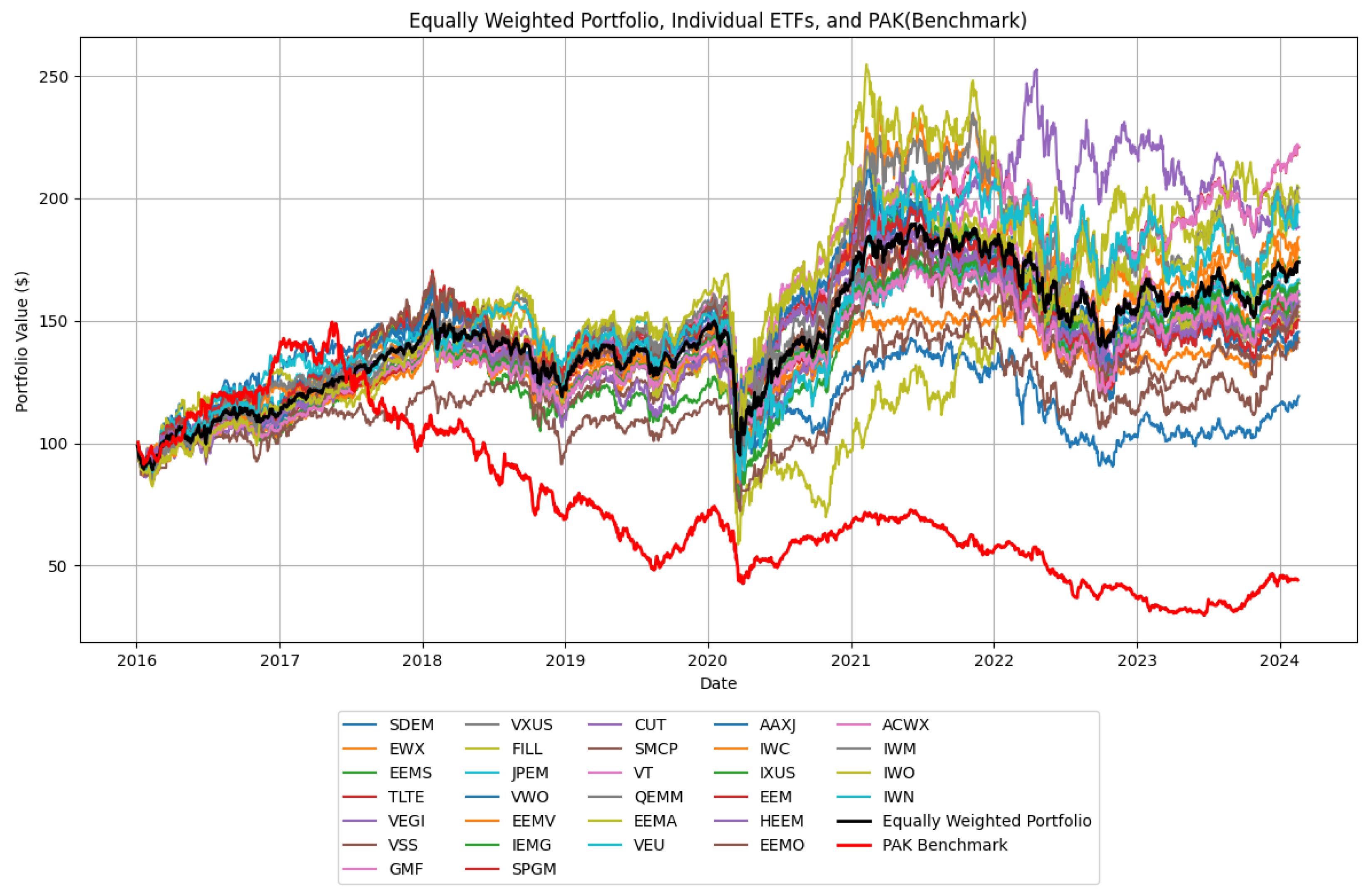
This section analyzes the different asset allocation tools institutional investment managers use to investigate the different risk–return profiles to accommodate various market environments and risk tolerances for the ETF presented in this paper. Given the performance comparison of the equally weighted portfolio (EQW) against PAK, the ETF with the highest exposure to Pakistan’s financial market, we conduct a historical analysis based on the method outlined in Lindquist et al. (2021). To investigate the performance of our portfolio, we construct an EQW and a Markowitz efficient frontier that is robust in conducting a historical analysis.

Using an EQW as a benchmark to analyze the historical performance of the PAK ETF (an exchange-traded fund with the highest exposure to Pakistan) offers a compelling approach that can be used to evaluate the risk and return profile of a concentrated, country-specific investment. An EQW, by definition (see Markowitz (1952) and Sharpe et al. (1999)), allocates an equal proportion of investment capital to each included asset, providing a neutral, diversified baseline. This benchmark does not favor any specific sector or country and thus stands as an effective comparison point for the single-country focus of PAK. Evaluating PAK against an EQW allows an assessment of how concentrated exposure to Pakistan’s market measures up against a diversified strategy, especially regarding the risk, return and volatility.

In this section, we will consider the performance of the optimizations on the portfolio of 30 ETFs under a long-only strategy and a basic long-short strategy. Weights for the individual ETFs are determined based on the returns from a rolling window of 1008 trading days (four trading years). The time window will give us a sample large enough to create a feasible set of values of weights. After constructing complete time series of optimized portfolio weights, we computed performance measures. We are not following historical optimization for the weights of EQW; instead, the weights are computed based on the equal weighting of the prices of the assets in the portfolio on the previous day.

3.1. Basic Strategies, Price and Return Performance

3.1.1. Long Only

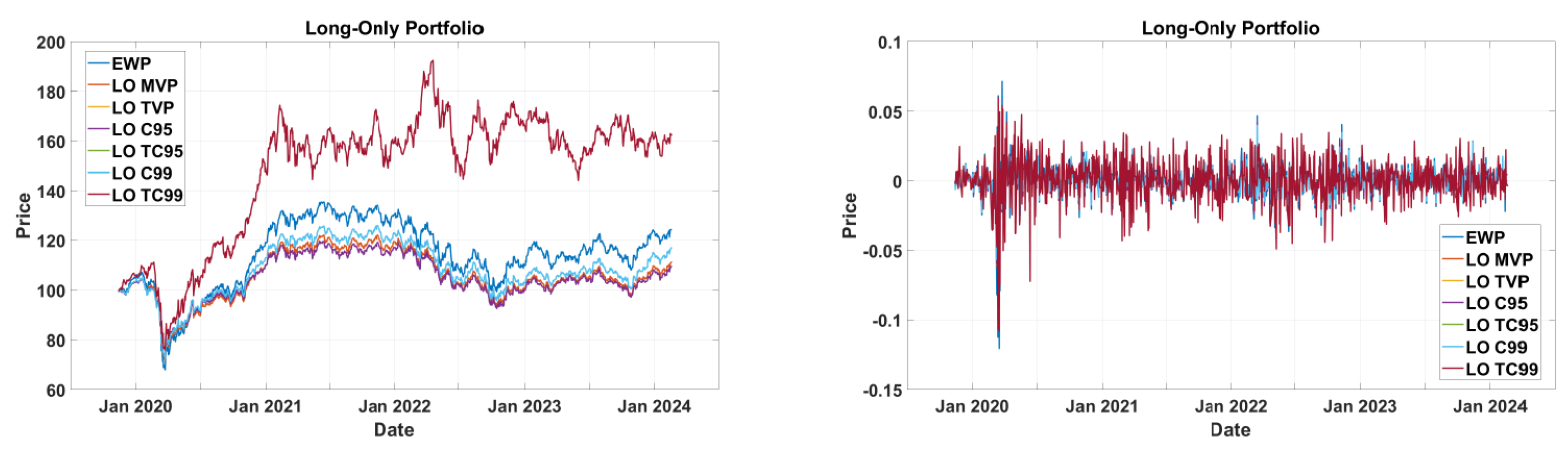
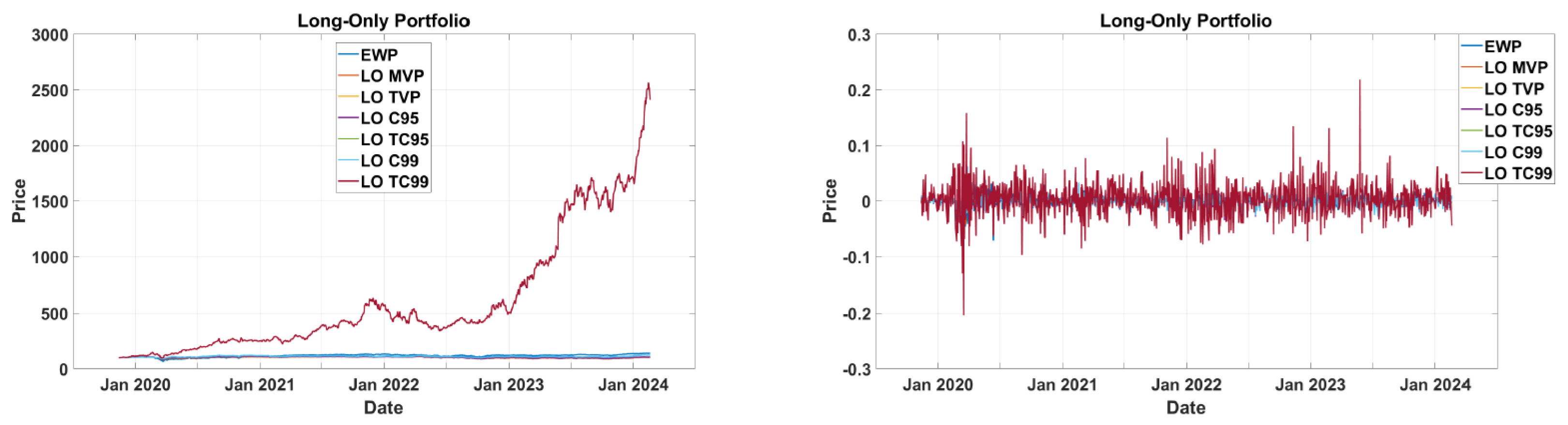
The performance of the cumulative price of each portfolio from 13 November 2019 through 19 January 2024, assuming a $100 investment in the portfolio on 12 November 2019, is shown in Figure 2. As shown by the plot, tangent portfolios, including the time-varying portfolio (TVP), T95 and T99, outperform all the others. The minimum variance portfolio (MVP) and C95 strongly track each other. Interestingly, the unoptimized EQW portfolio performs rather well, most noticeably in the post-crisis period from 2021–2024. However, in the long term, it underperforms the tangent portfolios while outperforming the global risk-minimizing portfolios.

3.1.2. Long Short

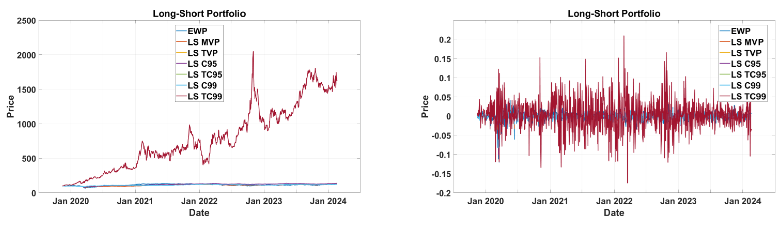
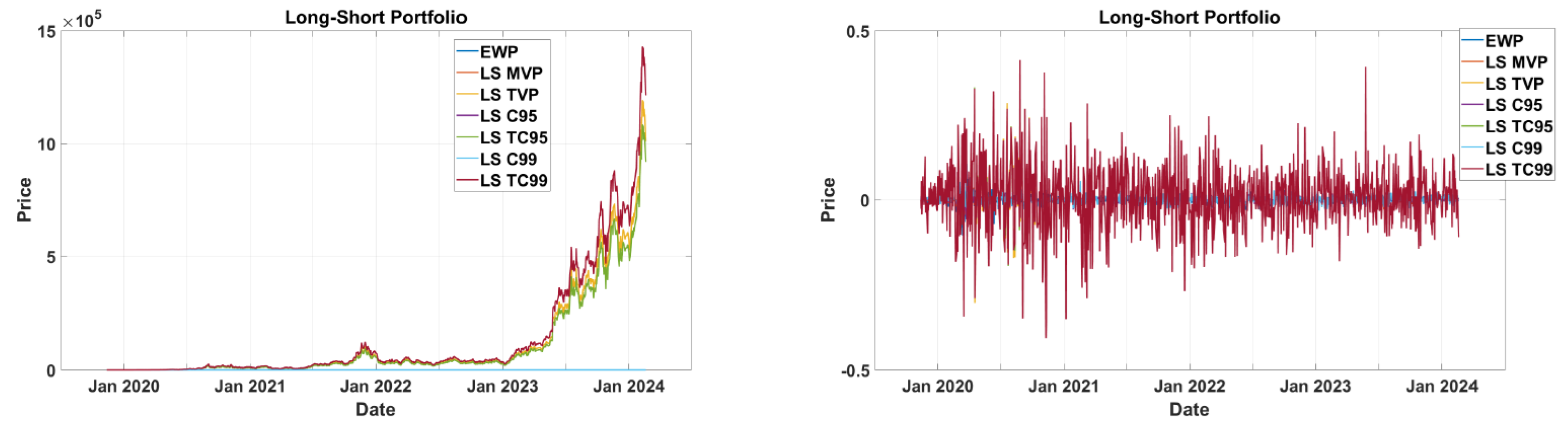
The evaluation of long-short portfolios constructed using 30 ETFs with an initial investment of $100 reveals distinct risk–return trade-offs. Figure 3 shows that long-short (LS) TC99 portfolio significantly outperforms the others, showcasing its strong growth potential. However, this portfolio exhibits substantial volatility, as evidenced in the right panel. Portfolios like LS C95 and LS TC95 offer moderate returns with relatively low volatility, striking a balance between risk and reward. On the other hand, more conservative strategies such as the EQW, LS MVP and LS TVP show stable performance but limited growth, barely exceeding the baseline. These strategies are well-suited for risk-averse investors prioritizing capital preservation over returns. The right panel emphasizes that aggressive portfolios like LS TC99 (long-short tracking constraint 99%) and LS C95 have highly volatile returns, whereas the EQW and LS MVP deliver stable, consistent returns. Overall, LS TC99 offers the highest returns at the cost of significant volatility, while the EQW and LS MVP prioritize stability for conservative investors.

3.2. Key Performance Ratios

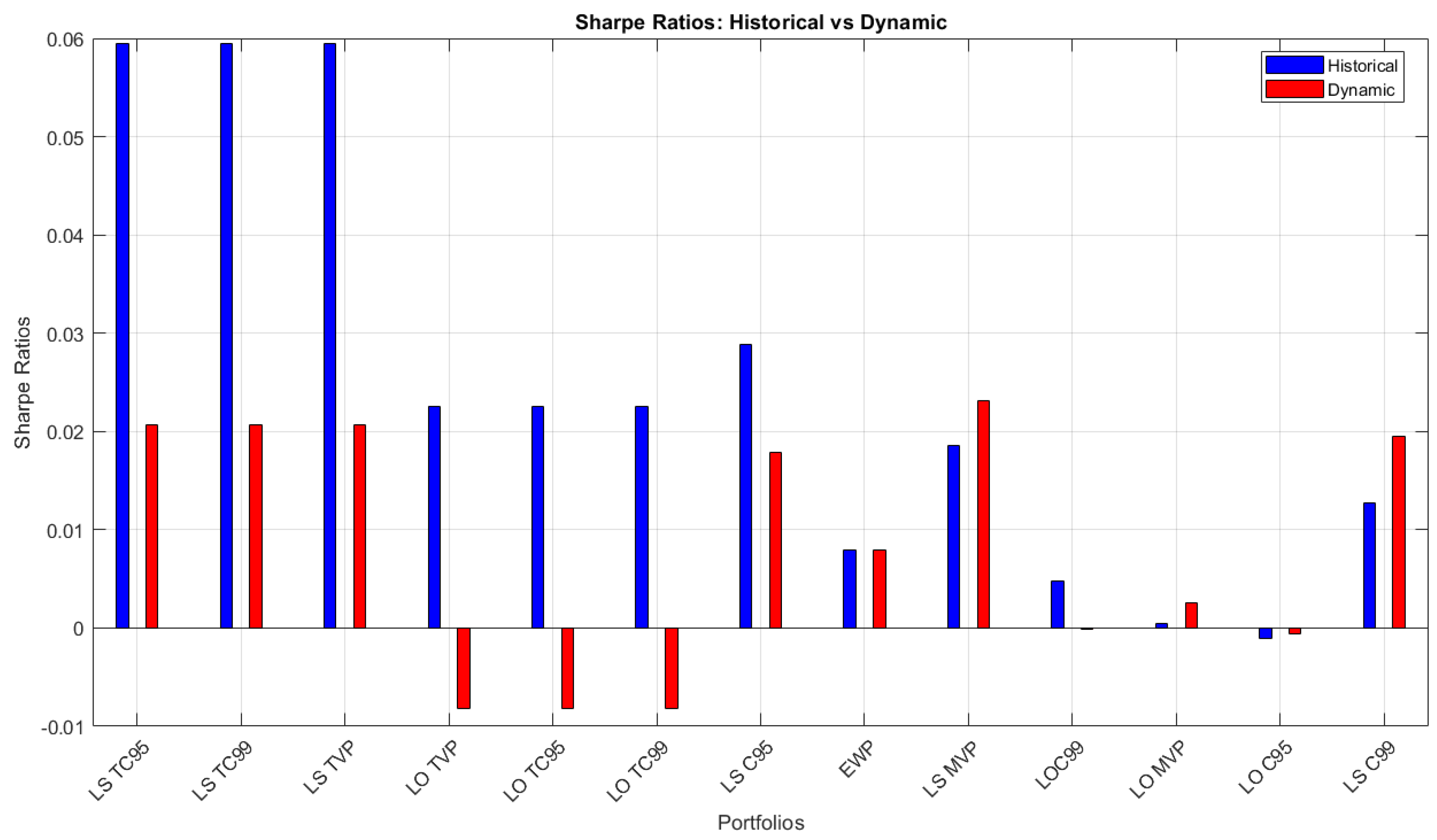
Figure 4 illustrates the time evolution of the Sharpe ratios for various portfolios, computed using a one-year moving window. LO MVP, LS MVP portfolios are constructed to maximize the Sharpe ratio under the traditional mean-variance framework. While they perform well in stable conditions, they exhibit a significant decline during periods of heightened volatility, reflecting their sensitivity to changing market dynamics. LO TVP, LS TVP Sharpe ratios exhibit higher variability, indicating responsiveness to market shifts. LO C95, LO C99, LS C95 and LS C99 portfolios incorporate downside risk constraints by optimizing under CVaR conditions at 95% and 99% confidence levels. Notably, they maintain higher Sharpe ratios during market downturns, suggesting superior resilience against extreme losses. The 99% CVaR portfolios (LO C99, LS C99) demonstrate stronger stability compared to their 95% counterparts. LO TC95, LO TC99, LS TC95 and LS TC99 exhibit relatively smoother trends, suggesting enhanced robustness in volatile environments (See Appendix A).

Table 4. Maximum Drawdowns of Portfolios.

Portfolio	Max. Drawdown
LS_TC95	0.591018918
LS_TC99	0.591018918
LS_TVP	0.591018918
EQW	0.365943773
LO_TVP	0.317027745
LO_TC95	0.317027745
LO_TC99	0.317027745
LO_MVP	0.313304961
LO_C99	0.308339959
LO_C95	0.303296926
LS_MVP	0.239419095
LS_C95	0.191313723
LS_C99	0.158217606

shows the maximum drawdowns (MDDs) of various portfolios, with the highest MDD of 0.591 observed in long-short TC95, TC99 and TVP, indicating that these portfolios are the most vulnerable to peak-to-trough declines, likely due to aggressive strategies or higher risk exposure. In contrast, long-short C99 exhibits the lowest MDD at 0.158, showcasing superior resilience and effective risk control. Portfolios like the EQW (MDD 0.366) and the long-only portfolios (MDD ranging from 0.317 to 0.303) offer moderate risk profiles, balancing returns and vulnerability.

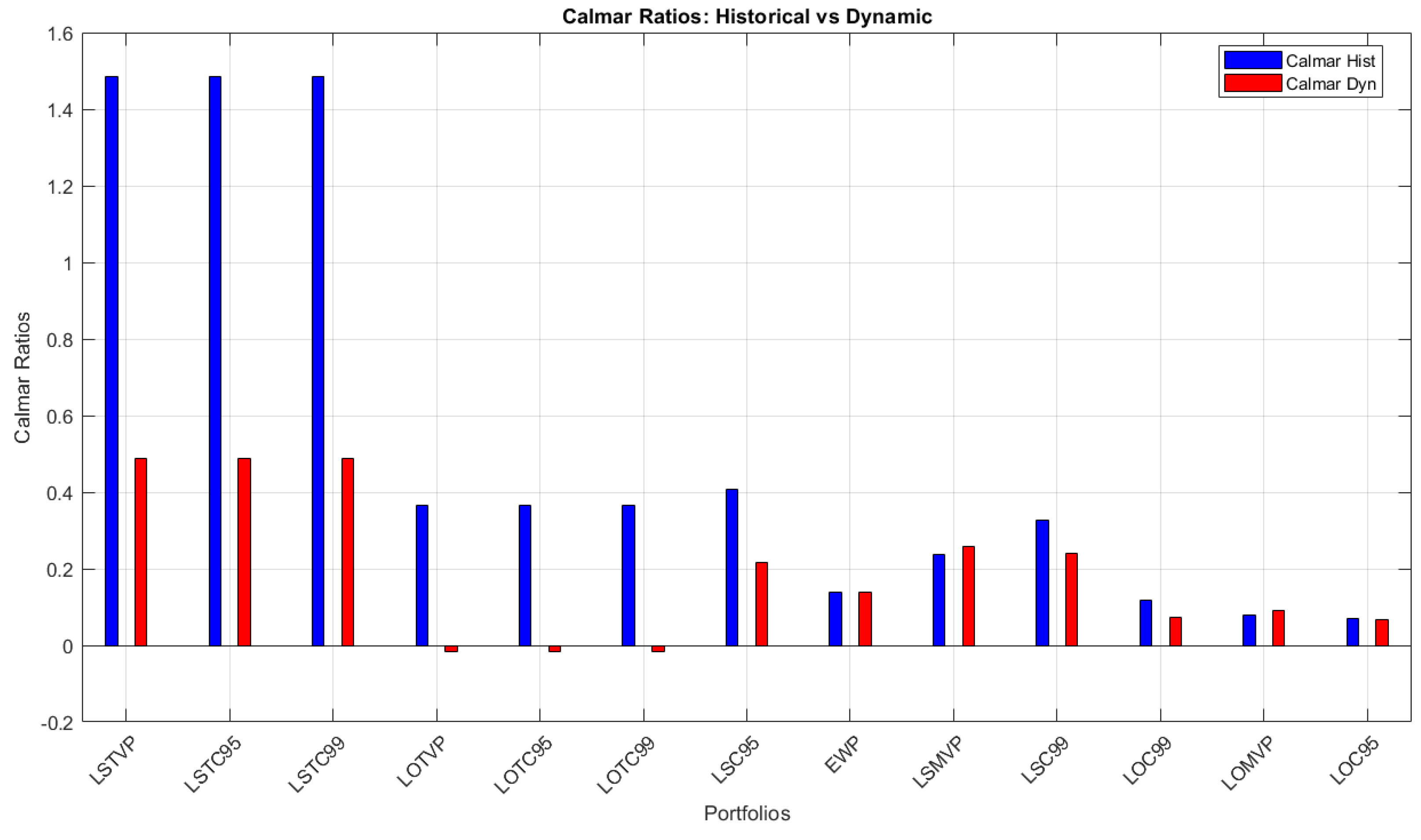
As we can observe in

Table 5. Calmar Ratios of LS and LO Portfolios.

Portfolio	Calmar Ratio
LS TVP	1.486
LS TC95	1.486
LS TC99	1.486
LS C95	0.406
LO TVP	0.365
LO TC95	0.365
LO TC99	0.365
LS C99	0.326
LS MVP	0.237
EQW	0.138
LO C99	0.118
LO MVP	0.079
LO C95	0.070

long-short (LS) portfolios dominate in terms of performance, with the TVP, TC95 and TC99 achieving the highest Calmar ratio of 1.486, indicating that these portfolios generate the highest return relative to their drawdown risk. This suggests that they are exceptionally efficient in balancing returns and risks. Among the remaining LS portfolios, C95 has a Calmar ratio of 0.406, followed by C99 at 0.326 and the MVP at 0.237, showing a gradual decline in efficiency.

The long-only (LO) portfolios exhibit significantly lower Calmar ratios, with the TVP, TC95 and TC99 clustered at 0.365, suggesting moderate performance. Other LO portfolios, such as C99 (0.118) and C95 (0.070), have the lowest Calmar ratios, indicating less efficient risk-adjusted returns. The EQW, with a Calmar ratio of 0.138, performs slightly better than the least efficient LO portfolios but remains significantly below the top-performing LS portfolios. This analysis highlights that LS strategies, particularly the TVP, TC95 and TC99, provide superior risk-adjusted returns compared to LO portfolios.

Table 6. STARR Values of LS and LO Portfolios.

Portfolio	STARR
LS TVP	1.059
LS TC95	1.059
LS TC99	1.059
LS C95	0.622
LS MVP	0.440
LO TVP	0.361
LO TC95	0.361
LO TC99	0.361
LS C99	0.257
EQW	0.165
LO C99	0.141
LO MVP	0.097
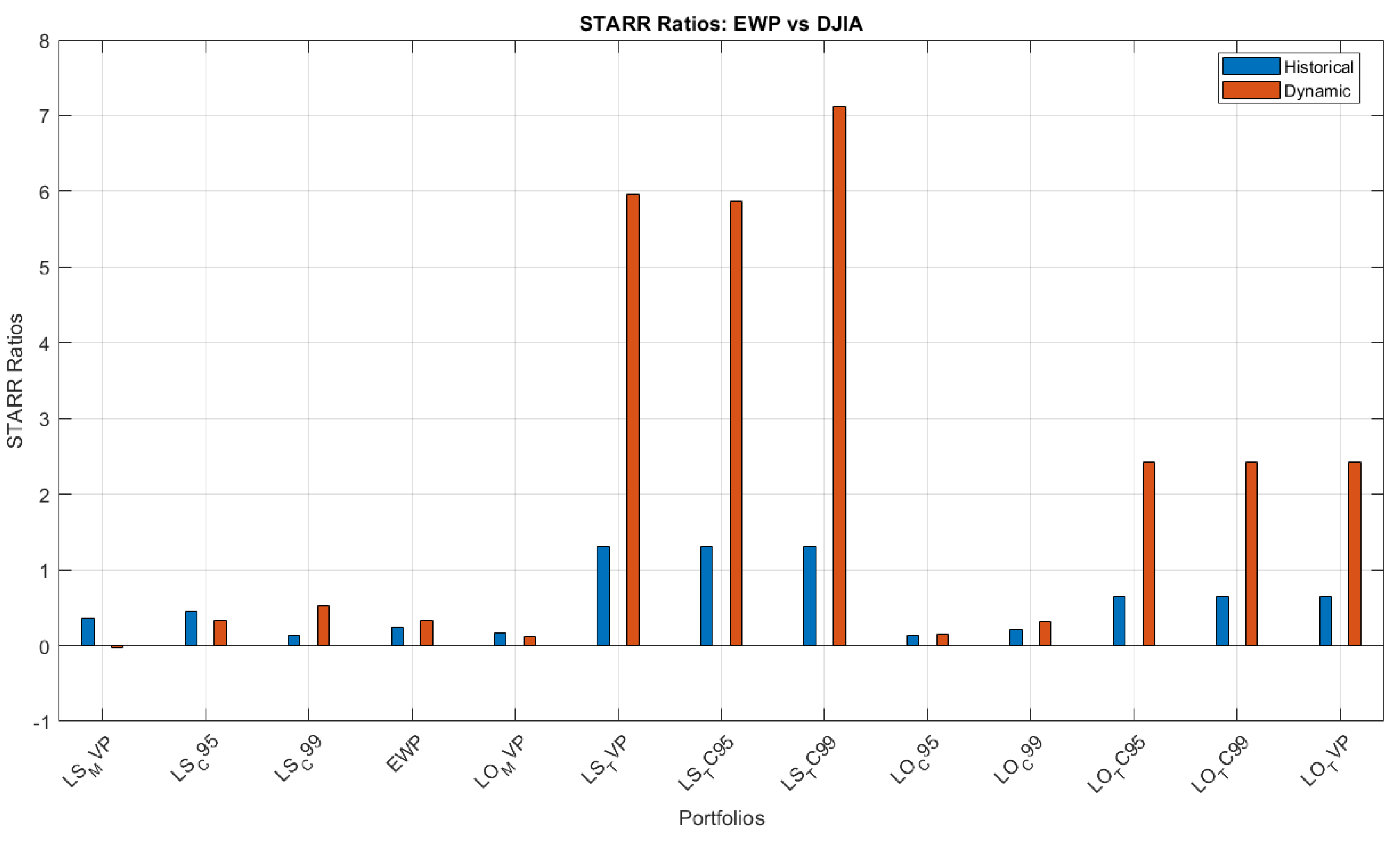
LO C95	0.083

presents the stable tail adjusted return ratio (STARR) values for various portfolios; they measure the risk-adjusted performance considering the tail risk. The LS portfolios consistently outperform the LO portfolios. LS TVP, LS TC95 and LS TC99 achieve the highest STARR value of 1.059, showcasing a superior tail-risk-adjusted performance. LS C95 follows with a STARR of 0.622, and LS MVP has a STARR of 0.440, with both maintaining a clear advantage over LO portfolios. Among the LO portfolios, the TVP, TC95 and TC99 exhibit identical STARR values of 0.361, representing moderate performance. The lowest-performing portfolios include LO C99 (0.141), LO MVP (0.097) and LO C95 (0.083), indicating weaker returns relative to their tail risks. The EQW sits between the LS and LO portfolios with a STARR of 0.165. This analysis highlights that LS strategies, particularly the TVP, TC95 and TC99, are optimal for tail-risk-conscious investors, while LO portfolios show a lower risk-adjusted efficiency. Other key performance ratios are in the Appendix A

In the context of Pakistan-exposed ETFs, these performance metrics are especially critical. The Sharpe ratio assesses overall risk-adjusted performance, the Calmar ratio highlights the importance of managing drawdowns in volatile frontier markets, and the STARR provides a measure of tail-risk-adjusted returns—crucial given the potential for sudden economic and political shocks. The Sharpe ratio is not a proper performance measure as it fails to satisfy the monotonicity axiom. Additionally, sigma, which is used in the Sharpe ratio, is not a coherent risk measure. In contrast, the stable tail adjusted return ratio (STARR) satisfies all four axioms of coherent risk measures —monotonicity, quasi-concavity, scale-invariance, and distribution-based properties—as established in Cheridito and Kromer (2013). Importantly, the STARR effectively accounts for tail risk, ensuring that extreme market scenarios are adequately captured in performance evaluation.

3.3. Tail Risk Comparison

In this section, we will compare the tail risk using the Hill estimator. The Hill estimator is often used to estimate the tail index of financial indices. The purpose is to comprehend the probability of extreme losses or gains and investigate the distribution of the tails. For this study, we focus on the following comparisons:

• Equal-weighted portfolio (EQW) vs. Dow Jones Industrial Average (DJIA);
• Global X MSCI Pakistan ETF (PAK) vs. S&P 500.

As we can see from Figure 5, the EQW has a higher initial Hill estimator value compared to the DJIA, indicating a potentially heavier tail for the initial order statistics. This could mean that extreme events in the EQW are more pronounced compared to those in the DJIA, possibly due to the equal-weighted nature of the portfolio, which might introduce more variability. As the number of order statistics increases, both the EQW and DJIA show a stabilization in their Hill estimators, converging towards a steady estimate. However, the EQW exhibits more fluctuation early on compared to the DJIA, suggesting that the DJIA may have more stable tail behavior.

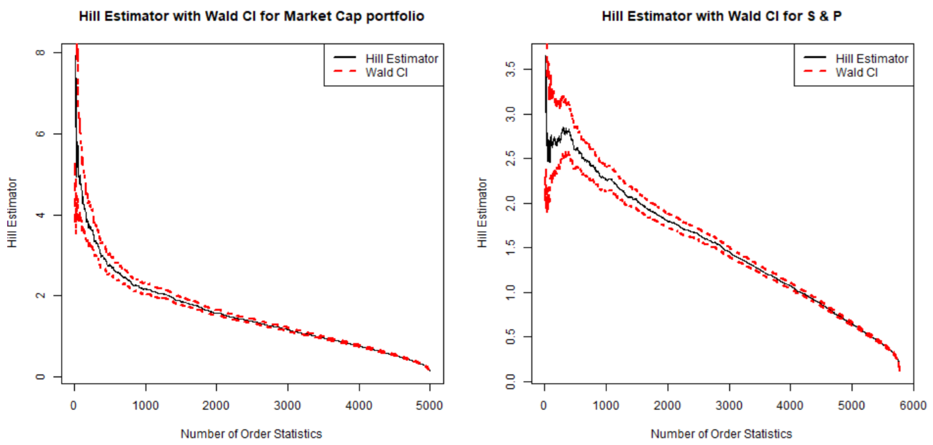
Similarly, in Figure 6, the Hill estimator for the S&P 500 is notably lower compared to the market cap portfolio. It starts around a value of 3.5 and then gradually decreases and stabilizes as more order statistics are included. This lower value indicates that the S&P 500 has a lighter tail compared to the market cap portfolio, implying fewer extreme events in the distribution of returns. The Wald confidence interval for the S&P 500 is initially wider but narrows more quickly than that of the market cap portfolio. This suggests that the tail estimation for the S&P 500 becomes more reliable with fewer extreme values, indicating a more stable tail distribution.

3.4. Markovitz Efficient Frontier

In the method introduced by Markowitz (1952), the objective of portfolio optimization is to determine the set of asset weights that minimize the portfolio return risk, given a desired level of expected portfolio return ${\tilde{r}}_p$. The target value of ${\tilde{r}}_p$ reflects the investor’s risk tolerance; a higher ${\tilde{r}}_p$ indicates a greater willingness to accept risk. Using the portfolio variance ${\sigma }_p^2$ as a measure of risk, Markowitz’s mean-variance optimization framework seeks to minimize this variance, subject to constraints on the expected return and ensuring full investment across all assets. Formally, this can be expressed as the minimization of the portfolio variance under the constraints of the desired expected return and total allocation of investment capital.

We follow the Markowitz mean-variance portfolio optimization problem, as outlined in Lindquist et al. (2021). The optimization problem is solved using standard methods of employing Lagrange multipliers:

$$\underset{w,q,{\theta }_0}{min}L(w,q,{\theta }_0)=\underset{w,q,{\theta }_0}{min}({\displaystyle \frac{w^T\Sigma w}{2}}+q({\overline{r}}_p-{\overline{r}}^{T}w)+{\theta }_0(1-e_n^{T}w)).$$

(1)

Taking the first-order conditions yields the following optimality conditions for w:

$$w^{\ast }={\overline{r}}_p{w}_1+w_2,$$

(2)

and the variance of the portfolio is given by

$${\sigma }_p=\sqrt{w^{\ast T}\Sigma w^{\ast }}=\sqrt{{\displaystyle \frac{B{\overline{r}}_p^2-2C{\overline{r}}_p+A}{\Delta }}}$$

where $A={\overline{r}}^T{\Sigma }^{-1}\overline{r}$, $B=e_n^T{\Sigma }^{-1}{e}_n$ and $C={\overline{r}}^T{\Sigma }^{-1}{e}_n$. Therefore, $\Delta =AB-C^2$. Given these relationships, $({\sigma }_p\left(w^{\ast }\right),{\overline{r}}_p)$ are the portfolio frontier points that trace out a hyperbola in the risk (standard deviation) and return (mean) space.

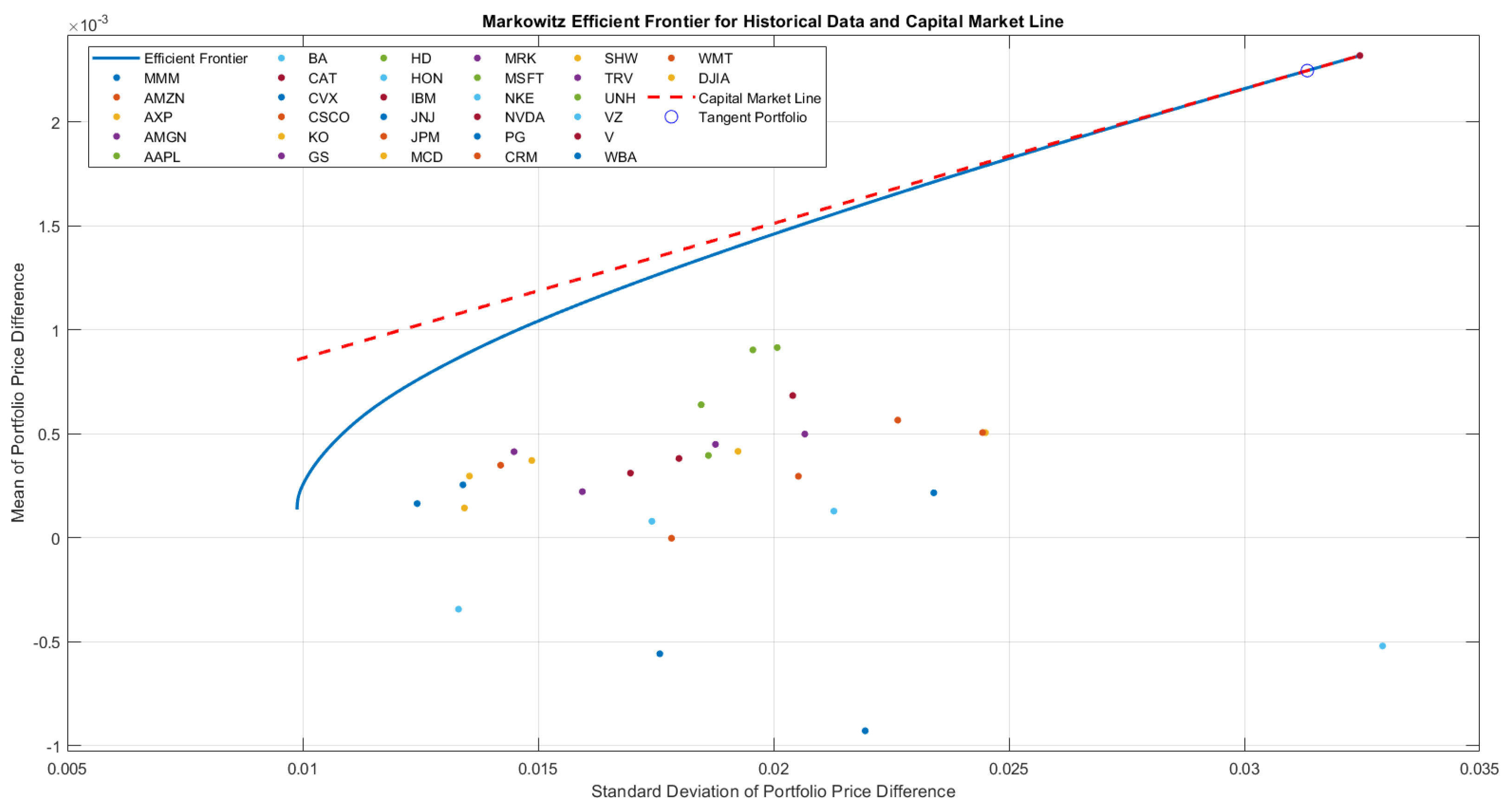
Figure 7 shows the Markowitz efficient frontier for a set of portfolios composed of various assets, including the EQW and PAK ETFs, along with other ETFs. The efficient frontier represents the set of portfolios that offer the highest expected return for a given level of risk or the lowest risk for a given level of return. The red dashed line is the capital market line (CML) that represents the risk–return trade-off for portfolios that combine a risk-free asset with the market portfolio. The point where the CML intersects the efficient frontier represents the tangency portfolio, or the optimal market portfolio, which maximizes the Sharpe ratio. Each dot represents the risk and return profile of a single ETF. The scattered positions indicate a variety of risk–return trade-offs across the ETF options. The EQW is closer to the efficient frontier, making it a relatively efficient choice among the ETFs, providing a good risk–return balance. PAK lies below the efficient frontier, indicating that it is an inefficient choice in this risk–return space; investors are exposed to more risk than necessary for the return PAK offers. The Markowitz efficient frontier framework is applied to evaluate the risk–return efficiency of selected ETFs in our study. By mapping EQW and PAK ETFs onto the efficient frontier, we assess their relative efficiency in portfolio construction. This analysis helps determine whether these ETFs provide optimal diversification benefits compared to other options. Specifically, EQW’s position near the efficient frontier suggests it offers a competitive risk–return profile, while PAK’s placement below the frontier indicates inefficiency. This finding is relevant for investors seeking optimal portfolio allocations in emerging markets.

The Markowitz efficient frontier serves as a foundational benchmark for evaluating the performance of portfolios that incorporate Pakistan-exposed ETFs. By constructing the efficient frontier, the study enables a systematic assessment of the trade-offs between risk and return, which are central to portfolio optimization. The efficient frontier is derived from modern portfolio theory (MPT), where the optimal portfolios maximize expected returns for a given level of risk or minimize risk for a given expected return. In the context of Pakistan-exposed ETFs, this framework provides an intuitive visual representation of diversification benefits and the relative efficiency of different portfolio configurations.

By plotting portfolio allocations along the efficient frontier, investors can identify optimal risk-adjusted strategies, comparing them against equally weighted portfolios. This comparison underscores the importance of portfolio diversification, particularly in an emerging market context where volatility and market inefficiencies may be more pronounced. By incorporating this methodological approach, the study provides a rigorous empirical foundation for assessing the relative performance of Pakistan-exposed ETFs. This, in turn, contributes to broader discussions on emerging market portfolio construction, offering insights into risk mitigation strategies and return enhancement techniques within the framework of global asset allocation.

4. Dynamic Portfolio Optimization

The historical optimization approach, as described and further demonstrated in the previous section, involves sequentially sampling return data using a rolling window technique over a fixed historical period that captures a finite range of market conditions. However, as is often highlighted in fund prospectuses, historical performance does not necessarily predict future outcomes. Instead of relying solely on historical asset return samples, dynamic optimization aims to enhance the insights that can be extracted from historical data. This approach assumes that historical returns originate from a dynamic multivariate distribution—dynamic in the sense that its statistical properties, such as covariance, may evolve over time. Dynamic optimization focuses on characterizing this distribution and generating extensive predictive samples of correlated asset returns, specifically aiming to capture more of the distribution’s tail behavior, including extreme events. The outcome is a portfolio optimization process that is better calibrated to anticipate significant shifts in market performance (Lindquist et al., 2021).

Pakistan’s market, as a frontier economy, is subject to abrupt changes in liquidity, policy, and macroeconomic factors, which significantly affect ETF returns. Dynamic optimization is particularly suited to such markets as it captures evolving volatility and correlation structures, enabling more adaptive portfolio construction than static historical models.

Historical optimization methods, such as those using a fixed rolling window, inherently assume that past market conditions provide sufficient information to guide future investment decisions. Dynamic optimization addresses these challenges by modeling asset returns as originating from a dynamic multivariate distribution. This approach ensures that the statistical characteristics of asset returns—such as mean, variance and correlation structures—are updated over time, improving the reliability of forecasts. For instance, the use of ARMA-GARCH models allows for a more realistic depiction of volatility clustering and persistence. Unlike traditional methods that rely solely on past return samples, dynamic optimization continuously updates its forecasting mechanism. This enables a more proactive portfolio adjustment strategy, aligning with findings that suggest dynamic rebalancing leads to superior performance in volatile markets (Brandt, 2010). The optimized portfolio weights are recalibrated daily based on updated risk–return trade-offs, ensuring that the investment strategy remains responsive to changing market conditions.

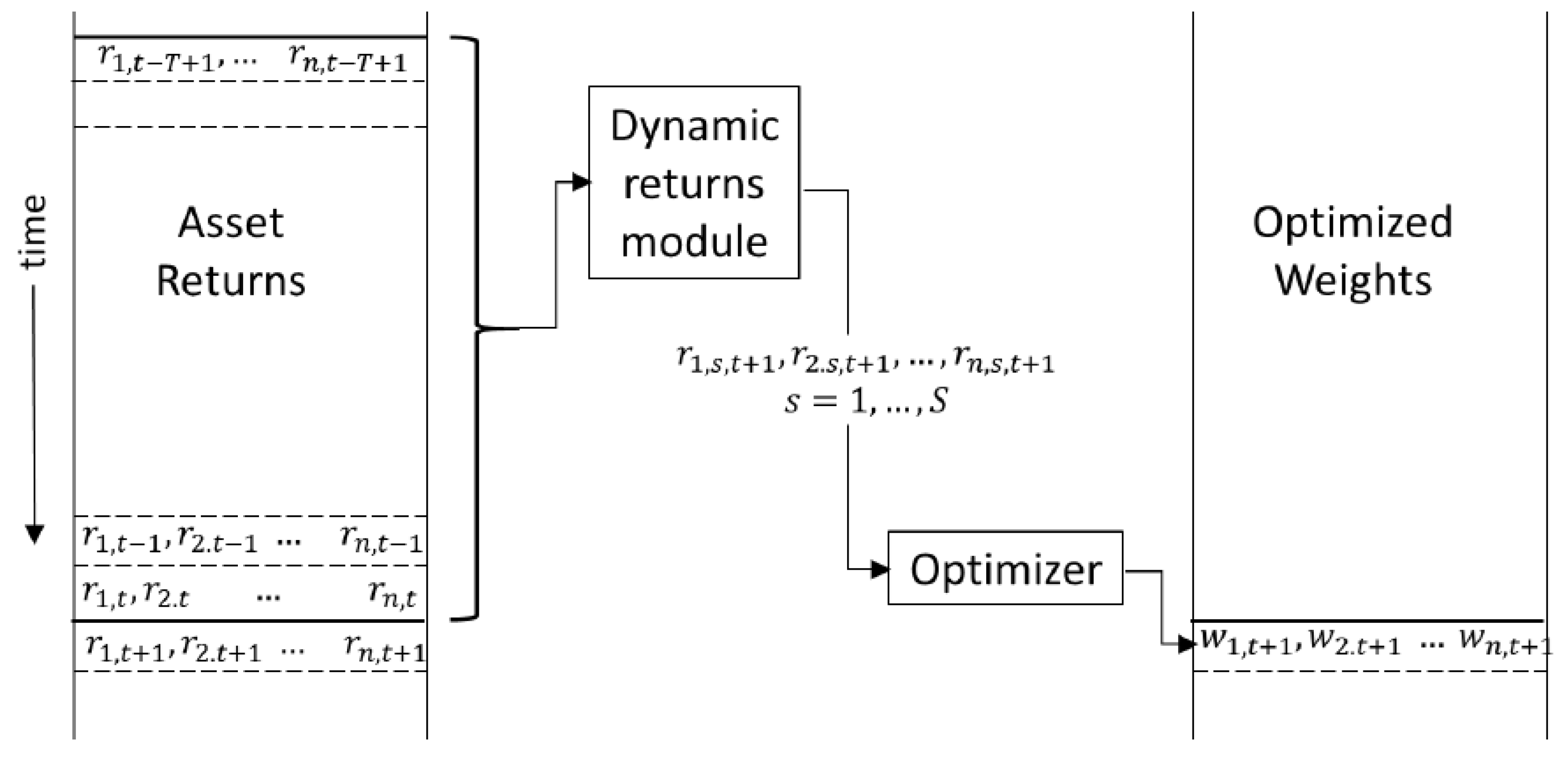
In this section, we implement dynamic optimization. There are some key parts of this optimization. In each rolling window, we will fit a common time series model, the ARMA(1,1)-GARCH(1,1) model, which will be referred to as the AG model, to the return data of the ETFs. In addition to that, a Student’s t distribution that takes into account extreme scenarios will be employed as an empirical model for the innovations in the AG fit. The process begins by transforming the data into a format where all parts of the distribution, including extreme values (tails), are treated equally. This is carried out using a “copula transformation”. After the transformation, the data are modeled using a multivariate copula, which captures how the assets move together (their correlations). Using this model, a large set of possible values for the asset movements is simulated. These simulated values are then converted back into their original format using an inverse transformation. Finally, these values are used to estimate a wide range of potential portfolio returns, which are then fed into the optimization process to determine the best asset weights for the next day. The main purpose of this optimization is to come up with a statistically correct large-sample process. We will achieve this in a way that uses the initial historical window of return data with a dynamic forecast of returns for the next day that will be utilized in the optimization for determining weights on day t + 1.

4.1. AG Model with Student’s t Distribution

We will use the empirical specification for the ARMA(p,q) model developed by Tsay (2005), and the ARMA(1,1)-GARCH(1,1) model will be defined as follows:

$$\begin{gathered} r_t={\delta }_0+\sum _{i=1}^p{\delta }_i{r}_{t-i}+{\alpha }_t+\sum _{j=1}^q{\delta }_j{\alpha }_{j-1}, \\ {\alpha }_t={\sigma }_t{ϵ}_t, \\ {\sigma }_t^2={\alpha }_0+{\alpha }_1{a}_{t-1}^2+{\beta }_1{\sigma }_{t-1}^2, \end{gathered}$$

where ${\alpha }_t$ is a shock. In this specification, our assumption is that the residuals ${ϵ}_t$ follow a Student’s t distribution:

$$t_{\nu }\left(x\right)={\displaystyle \frac{\Gamma \left(\frac{1+\nu }{2}\right)}{\sqrt{\nu \pi }\Gamma \left(\frac{\nu }{2}\right)}}{\left(1+{\displaystyle \frac{x^2}{\nu }}\right)}^{-{\displaystyle \frac{1+\nu }{2}}}.$$

(3)

where $\Gamma$() denotes the gamma function. The subject distribution is symmetric but relatively leptokurtic in comparison to the normal distribution. As shown in Figure 8, a window of historical returns is transformed into a dynamic set of returns, which are then passed to the portfolio-optimizing routine.

The selection of ARMA-GARCH models and the Student’s t distribution in our study is grounded in well-documented empirical evidence regarding the statistical properties of financial return. As outlined in Cont (2001), asset return distributions exhibit several key stylized facts that necessitate the use of these models. Cont (2001) highlights that the unconditional distribution of asset returns exhibits heavy tails that deviate significantly from the normal distribution. The Student’s t-distribution is particularly suited to modeling this feature because it allows for fatter tails, capturing extreme fluctuations in returns better than the Gaussian distribution.

One of the most critical properties of financial time series is volatility clustering, meaning that large returns (both positive and negative) tend to be followed by periods of high volatility. Cont (2001) emphasizes that volatility clustering leads to positive auto-correlations in squared returns that persist for several periods, a feature well modeled by GARCH-type processes. The empirical evidence presented by Cont (2001) strongly supports the choice of the ARMA-GARCH model with Student’s t-distributed errors. These models adequately capture key stylized facts of financial returns, such as heavy tails, volatility clustering, and nonlinear dependence, which are essential for accurately modeling return distributions and risk measures. By incorporating these features, our study ensures robustness in return modeling and aligns with best practices in empirical finance.

4.2. Basic Strategies, Price and Return Performance

4.2.1. Long Only

Figure 9 illustrates the performance of various portfolio strategies, starting with a $100 investment, from early 2020 to 2024. The EQW outperforms all other strategies, but it exhibits higher volatility, making it more suitable for risk-tolerant investors. Portfolios such as the MVP and TVP show moderate returns with lower volatility, offering a balanced approach for investors seeking steady growth. Overall, the EQW provides the best returns for aggressive investors, while the MVP and TVP are better suited for those with moderate risk tolerance. Conservative investors may need to reconsider TC99, as it fails to deliver adequate returns.

4.2.2. Long Short

The performance comparison of long-short portfolios in Figure 10 reveals significant differences in risk and return dynamics. The TC99 strategy emerges as the top performer, with aggressive growth, but it also exhibits high volatility, making it suitable for risk-tolerant investors. In contrast, conservative strategies like LS MVP and LS TVP demonstrate steady performance with low volatility, appealing to risk-averse investors. Portfolios such as LS C95 and LS TC95 offer a balance between risk and return, outperforming LS MVP and LS TVP while maintaining moderate volatility. Overall, LS TC99 is ideal for aggressive growth, while LS MVP and LS TVP cater to investors prioritizing stability.

4.3. Efficient Frontier

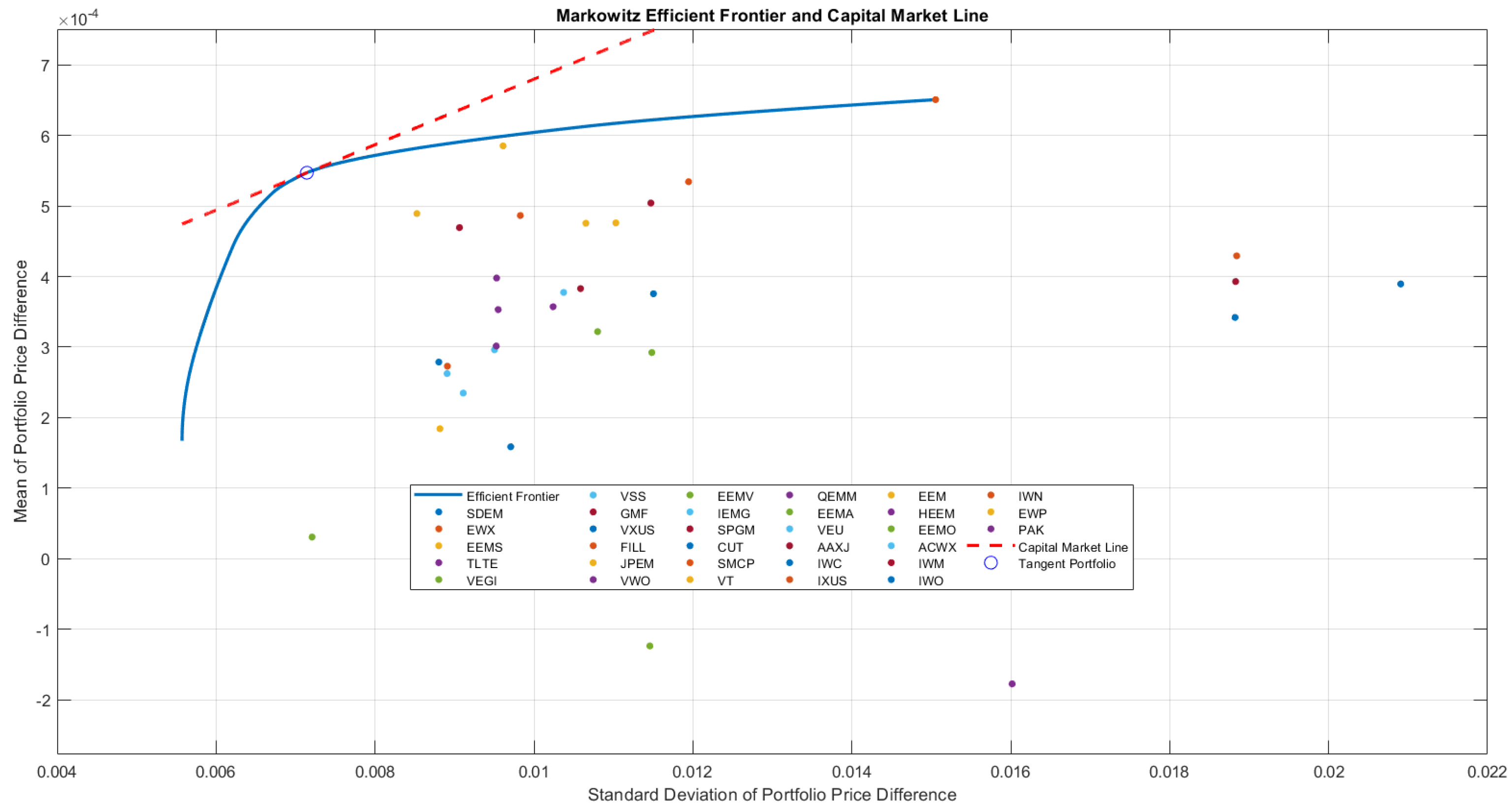
The Markowitz efficient frontier based on the dynamic optimization of 30 ETFs in Figure 11 shows the trade-off between risk (standard deviation of portfolio price differences) and return (mean of portfolio price differences). The efficient frontier (blue curve) highlights the portfolios that maximize returns for a given risk, while the CML indicates the optimal risk–return combinations when incorporating a risk-free asset. The EQW lies slightly below the efficient frontier, offering a balanced but suboptimal risk–return profile. In contrast, the Pakistan ETF (PAK) is inefficient, with higher risk and lower returns, demonstrating a poor risk-adjusted performance. The tangency point on the CML represents the market portfolio, offering the best possible risk–return trade-off. This analysis underscores the importance of diversification and optimization in portfolio construction to achieve superior risk-adjusted returns.

5. Dow Jones Industrial Average

5.1. Basic Strategies, Price and Return Performance

5.1.1. Long Only

The performance of the cumulative price of each portfolio with respect to the Dow Jones from 13 November 2019 through 19 January 2024 assuming a $100 investment in the portfolio on 12 November 2019, is shown in Figure 12. The portfolio TC99 exhibits exponential growth, far outperforming all other portfolios. This strategy, however, also displays substantial volatility. On the other hand, conservative portfolios such as LO MVP and LO TVP demonstrate a stable, low-risk performance, with minimal price growth and less variability, making them suitable for risk-averse investors. The EQW, which is the DJIA index, provides modest returns, performing better than LO MVP and LO TVP but significantly underperforming compared to LO TC99. Portfolios like C95 and TC95 strike a middle ground, achieving moderate growth with balanced risk. Overall, TC99 provides exceptional returns but at the cost of high risk, whereas the MVP and TVP cater to investors prioritizing stability over growth.

5.1.2. Long Short

Figure 13 shows the graphical analysis of long-short portfolios for the DJIA with an initial investment of $100 highlights notable differences in performance and risk profiles. The LS TC99 strategy demonstrates exceptional growth. This exponential growth, however, comes with significant risk, as seen in the high volatility reflected in the right panel. Other portfolios, such as LS C95 and LS TC95, also deliver impressive returns but with slightly lower growth trajectories compared to LS TC99. The EQW, LS MVP and LS TVP exhibit comparatively low returns and minimal volatility, making them better suited for risk-averse investors. The right panel further emphasizes that strategies like TC99 and C95 experience the highest levels of volatility, while the EQW and LS MVP remain stable. Overall, TC99 stands out for its exceptional return potential but involves significant risk, while the EQW, MVP and TVP provide stable but subdued growth for conservative investors.

5.2. Efficient Frontier

Figure 14 provides a clear visualization of the Markowitz Efficient Frontier and the Capital Market Line (CML) using historical data for DJIA, highlighting the optimal risk-return trade-offs for portfolio selection. The Dow Jones Industrial Average (DJIA) stocks, represented as scattered points, illustrate the individual risk and return characteristics of these assets before forming diversified portfolios. These stocks exhibit varying levels of risk (standard deviation) and return (mean price difference), with some positioned closer to the efficient frontier, indicating a more favorable risk-return profile, while others are further away, signifying higher risk with relatively lower returns.

6. Conclusions

The analysis of Pakistan-exposed ETFs highlights both the opportunities and challenges of investing in frontier and emerging markets. While Pakistan’s market exhibits unique characteristics, such as a low correlation with global markets and potential for diversification, the performance of ETFs like PAK reveals inefficiencies. Positioned below the efficient frontier, PAK offers lower returns for higher risk, making it suboptimal compared to diversified benchmarks like the EQW. However, the integration of Pakistan-focused ETFs into broader portfolios underscores their potential to mitigate risk through diversification, particularly for US investors seeking exposure to non-traditional markets. The findings demonstrate that while Pakistan’s structural challenges—such as political instability and market illiquidity—limit performance, the dynamic optimization framework offers pathways to enhance portfolio efficiency by capturing tail risks and adapting to evolving market conditions.

Dynamic optimization strategies, particularly those incorporating ARMA-GARCH models and Student’s t distributions, outperform historical approaches by effectively modeling risk and return trade-offs. Long-short strategies such as LS TC99 deliver superior returns, albeit with significant volatility, making them ideal for risk-tolerant investors, while conservative strategies like LS MVP and LS TVP cater to risk-averse preferences. The study underscores the critical role of advanced optimization techniques in managing the complexities of frontier markets, where traditional methodologies often fail to capture extreme events or evolving correlations. Overall, this research not only provides actionable insights for investors considering Pakistan-exposed ETFs but also contributes to the broader discourse on portfolio optimization in high-risk, high-reward markets.

Investors should use the CVaR ratio to detect warning signals of potential future market downturns. Market crashes, with few exceptions, are driven by fundamental changes in the economy, which do not occur overnight. Therefore, using CVaR to measure tail risk in relation to returns (CVaR ratio) is the appropriate metric for assessing the overall health of the economy.

For asset managers and institutional investors considering exposure to Pakistan through ETFs, this study highlights the importance of blending historical and dynamic optimization techniques to manage evolving risks. Employing long-short strategies for flexibility, integrating tail-risk awareness into portfolio construction, and monitoring dynamic correlations with global markets can significantly enhance risk-adjusted performance. Investors should also account for the structural characteristics of frontier markets, such as political volatility and liquidity constraints, when designing allocation strategies.

Future research should focus on advancing portfolio analytics for ETFs by addressing key emerging trends such as thematic and ESG ETFs, active ETFs, tokenized ETFs, and advanced risk management techniques. The increasing prominence of thematic and ESG ETFs underscores a shift toward sustainability and value-driven investing; however, concerns over higher fees and greenwashing persist Pástor et al. (2021). Similarly, the growing market for active ETFs challenges the traditional active–passive divide, yet their higher expense ratios often lead to underperformance relative to passive alternatives Ben-David et al. (2018). Additionally, tokenized ETFs leveraging blockchain technology offer enhanced transparency and liquidity, but regulatory ambiguity and cybersecurity risks hinder their widespread adoption Cong et al. (2022). To develop a comprehensive analytical framework for ETF performance assessment, future studies should examine the performance persistence of ESG ETFs and their sensitivity to macroeconomic shocks, explore the risk-adjusted returns of active ETFs across different market cycles and analyze the risk–return profiles of tokenized ETFs and their correlation with traditional asset classes. Moreover, research should prioritize liquidity metrics, bid-ask spreads, trading volumes and market impact analysis. The application of principal component analysis (PCA) can further aid in identifying hidden risk factors within ETF portfolios, enhancing risk management strategies. Given the evolving nature of ETFs, addressing these research gaps will provide valuable insights into risk–return trade-offs, ultimately guiding investors and policymakers in making informed financial decisions.