Application of a Slack-Based DEA Approach to Measure Efficiency in Public Sector Banks in India with Non-Performing Assets as an Undesirable Output

Abstract

Ignoring the presence of non-performing assets makes efficiency measurement inappropriate and incomplete. Thus, the present study considers non-performing assets as an undesirable output and applies the slack-based efficiency model to measure the efficiency of public sector banks in India during 2004–2005 to 2018–2019. A two-metric performance assessment of sample banks is carried out using mean efficiency and the non-performing assets management ratio. This study is extended to investigate determinants of bank efficiency using a fixed effects model and dynamic panel data regression on the contextual variables. Results show that profitability as measured by return on equity (ROE) and priority sector exposure have had no impact on efficiency. However, cost of deposits and capital adequacy ratio have a significant negative impact on the efficiency of public sector banks in India. Most importantly, the study finds a decline in efficiency in recent years, indicating a necessity of serious efforts for revamping these state-owned banks.

1. Introduction

Financial intermediation, which is key for real activity (Bernanke, 1983), helps transfer funds to the best use with the “highest social return” (Goldsmith, 1969) and promotes economic growth (Greenwood & Jovanovic, 1990). Financial intermediaries enjoy an advantage in terms of transaction costs and trading costs (Gurley & Shaw, 1960) and have the ability to signal where to invest on the basis of special knowledge that they possess (Leland & Pyle, 1977). They act as “delegated monitors” and overcome asymmetric information problems (Diamond, 1984), and facilitate risk transfer and financial sector participation (Allen & Santomero, 1998), among other roles performed by financial intermediaries in the entire superstructure of a nation’s economic system.

Among financial intermediaries, commercial banks play the most crucial role in the process of financial intermediation, fostering the process of economic development in both developed and developing economies (Čiković et al., 2023). Through the process of financial intermediation, they perform liability–asset transformation in addition to three other transformations, namely, size, maturity, and risk. Basically, banks transform illiquid assets into liquid assets that offer different, smoother returns (Diamond & Dybvig, 1983). It is noteworthy to mention here that financial intermediaries (including banks) have to select among competing sectors, firms, and investment projects (Stiglitz, 1989). This transfer of funds can result in a sub-optimal level of performance in the event of banks’ inability to screen and monitor loans effectively (Lowe, 1992) and ultimately leads to non-performing assets. Thus, banks are faced with the obligation to perform efficiently in order to survive in the long run (Bikker & Bos, 2008).

1.1. Non-Performing Assets (NPAs) as Undesirable Outputs in Efficiency Measurement

Efficiency is at the “core” of bank operations. Though not easy to define, the term “efficiency” may be used to refer to achieving the best possible output levels and/or using the least possible inputs. Bank efficiency is reduced not only due to higher inputs (or lower outputs), but also due to the existence of outputs that are “unwanted” or “undesirable” (also referred to as “bads”). One such “undesirable” output is non-performing assets (NPAs) in the case of banking. Although there is a vast literature on bank efficiency, the majority of researchers have ignored the existence of undesirable outputs. Fare et al. (1989) proposed that undesirable factors in performance measurement should not ignore undesirable outputs and should penalize “bads”. Their empirical analysis showed that performance rankings were found to be “very sensitive to whether or not undesirable outputs were introduced” in efficiency measurement. Recently, a few researchers have started recognizing the existence of undesirable outputs such as non-performing assets for efficiency measurement.

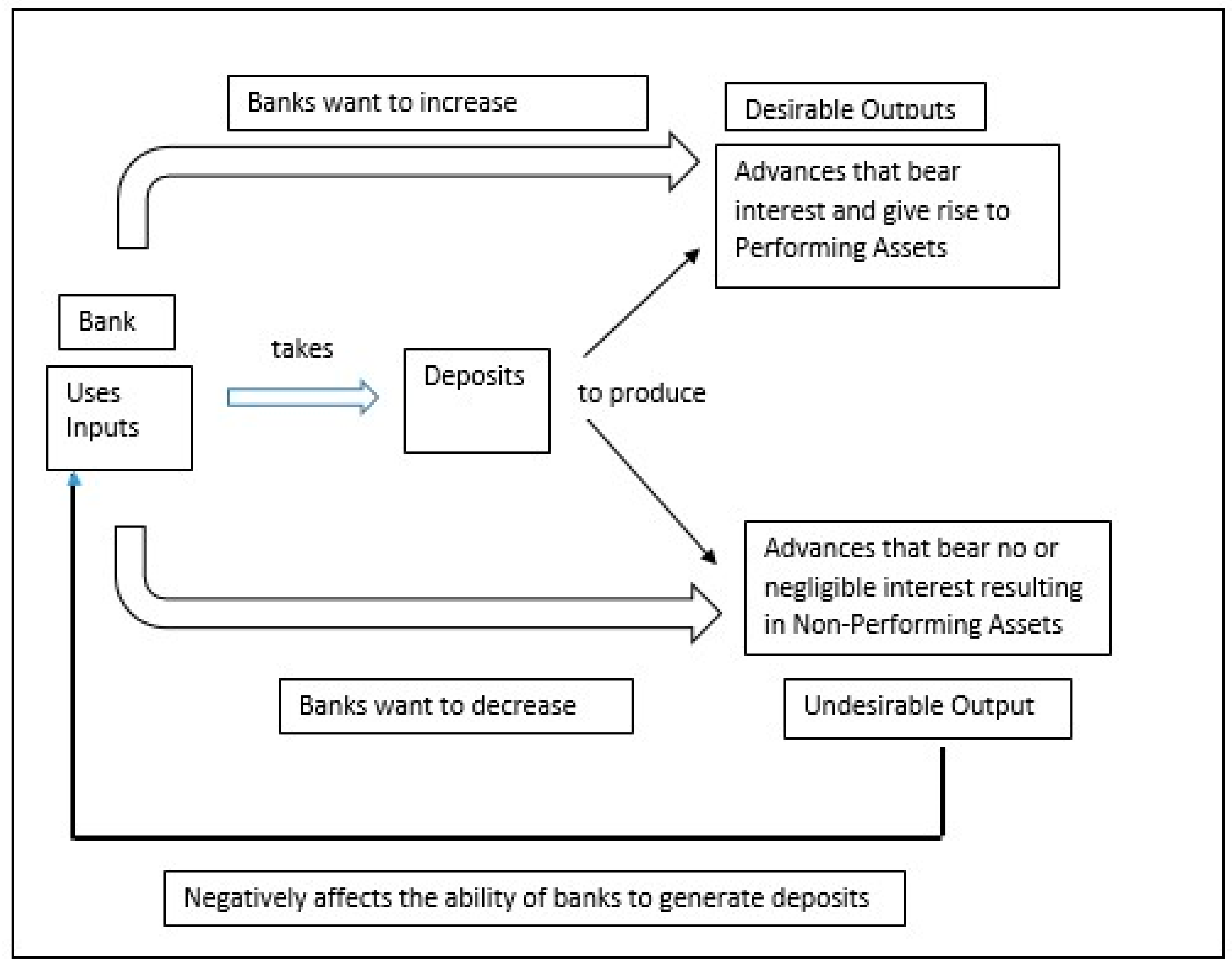
Banks take deposits from savers to produce advances to borrowers. The inability of banks to properly screen and select borrowers results in non-performing assets, thus giving rise to undesirable outputs together with desirable outputs. The creation of these undesirable outputs in the process of financial intermediation diminishes the ability of banks to generate deposits. Thus, it is in the banks’ interest that desirable outputs are increased and undesirable outputs reduced (refer Figure 1). By including NPAs as an undesirable output in the efficiency measurement of banks, researchers can avoid spurious efficiency scores.

The efficiency literature relating to the financial sector in general, and the banking sector in particular, has a rich heritage, as research outputs started to appear in the 1980s and early 1990s in the context of the US and European banking markets. Initial studies were based on econometric investigations and focused on X-efficiencies and allocative efficiencies, and the presence of economies of scale and scope in the banking sector. With the development of the non-parametric efficiency literature, the focus shifted towards the evaluation and explanation of the technical efficiency of the banking sector. However, the early evaluation models assumed that the banks only operate with desirable outputs that they seek to maximize (from an output-oriented standpoint). A major weakness of the desirable output framework is that it is not capable of accommodating the risk management approach in the efficiency evaluation framework, which is so crucial in view of the presence of credit risk as the dominant form of business risk in the commercial banking sector. In the efficiency evaluation stage, the present study seeks to recognize the existence of undesirable outputs in the banking sector with a view to remove the aforementioned weakness.

The use of an undesirable output model for efficiency evaluation commenced with the introduction of non-efficiency evaluation methods, as the econometric methods of investigation are incapable of handling multiple outputs. Fare et al. (1989) proposed that undesirable factors in performance measurement should not ignore undesirable outputs and should penalize “bads”. Their empirical analysis showed that performance rankings were found to be “very sensitive to whether or not undesirable outputs were introduced” in efficiency measurement. Inter alia, notable DEA-based efficiency studies include Fare and Grosskopf (1995, 2003, 2004), Scheel (2001), Seiford and Zhu (2002), and Tone (2004).

1.2. Public Sector Banks (PSBs) in India

The genesis of state-ownership of banks in India can be traced to the need to have a strong banking structure “to stimulate banking development in general and rural credit in particular” after Indian Independence in 1947. The Government of India took over the Imperial Bank of India (and renamed it the State Bank of India), and also took over the banks owned by princely states to make them subsidiaries of the State Bank of India, thus starting the era of “planned” banking in India. The aim of these state-owned public sector banks (PSBs) was “social control” by redirecting flow of bank credit from big industrial houses towards rural unbanked areas, agriculture, and small industries. Fourteen major banks, followed by six more banks, were nationalized in 1969 and 1980, respectively; this made PSBs the most dominant vehicle of financial intermediation in the country in terms of number of branches, mobilization of savings, and amount of credit disbursement. The government as the “owner, regulator and the sovereign” of PSBs introduced the directed lending or the priority sector lending programs for extending the reach of the Indian banking sector to the neglected sections of the economy, in addition to financing strategic industries.

In the last decade, numerous writers studied the efficiency of both public and private sector banks in the Indian context. However, any comparisons between PSBs and private sector banks are not valid and hence would lack any meaningful interpretation. PSBs are significantly different from their domestic private counterparts due to numerous reasons such as government ownership, objective of social justice, directed lending, development and political goals, and strict government oversight. Moreover, PSBs enjoy the benefits of government support in the form of recapitalization and restructuring, unlike private banks. Herwadkar et al. (2022) described three main roles of PSBs. First, PSBs are created to address market failures and their social benefits are higher than their costs (Atkinson & Stiglitz, 1980). Second, lending by PSBs is “countercyclical or less procyclical”. Third, PSBs have the maximum number of rural branches and provide credit to the rural population, contributing to the objective of financial inclusion. Private sector banks, on the other hand, operate with the sole objective of generating an economic surplus (except for the mandatory prudential norms and directed lending that must be followed). Thus, our study considers only the public sector banks for efficiency evaluation and estimation for two main reasons. First, because of the differences in the nature of ownership, there are major limitations regarding the comparison of bank technical efficiency across the public and private sector banks. Second, during the period under consideration, public sector banks experienced two major developments, namely, (i) the buildup of NPAs in the post-global financial crisis period; and (ii) the consolidation of banks within the public sector group, leading to a decline in the number of public sector banks from 20 to 12. The present study evaluates the performance of Indian PSBs for the pre-consolidation phase (2004–2005 through 2018–2019) using the slack-based model introduced by Tone (2004), taking non-performing assets as undesirable outputs, and then uses the estimated efficiency scores to explain bank profitability. Further, our study concentrates on the performance of three categories of public sector banks (acquired banks, acquirer banks, and the remaining banks, which were not involved in this consolidation process). For this, the study uses a two-stage approach. In the first stage, we estimated efficiency performance of the in-sample public sector banks with a special focus on the three categories of banks. In the second stage, we explored the influence of six contextual variables on the estimated efficiency scores.

This study has seven sections and proceeds as follows. Section 2 provides an overview of the Indian banking sector, the recurrence of the NPA problem in the banking sector, and consolidation of public sector banks. Section 3 reviews the research literature, identifies the research gaps, and specifies the major research questions. Section 4 describes the efficiency evaluation methodology. Section 5 describes the variables and data sources and discusses the results. Section 6 concludes, lists the limitations, and provides the scope of future research.

2. Banking Sector in India: Trends in Non-Performing Assets (Asset Quality) and Bank Consolidation

In India, the banking sector is the most important component of financial sector and has witnessed significant transformation since the latter part of the 1990s as a result of a process of globalization, deregulation, technological advancements, and reoriented regulatory and supervisory polices. Today, it is characterized by higher operational autonomy, stronger competitive pressures, and dynamic customer demands, which have resulted in financial innovations and diversified portfolios. Although the aim of this revamping was to shape an environment conducive for increased efficiency in bank operations, the banking sector witnessed an upsurge in non-performing assets, more so and intermittently in the public sector banks (PSBs). In the past three decades, Indian public sector banks witnessed two phases of sharp deterioration in banking sector asset quality: the first phase was during 1997–2002 and the second phase was during 2009–2019.

Even in the post-liberalization phase, public sector banks (PSBs) in India continue to have a major share in the consolidated balance sheet of scheduled commercial banks (SCBs) both in terms of deposits mobilized and assets held, although this share has been decreasing over the years. At the end of March 2019, public sector banks accounted for 65.85% of total deposits and 61% of total assets of scheduled commercial banks. Also, non-performing assets (NPAs) of public sector banks were higher than those of the other scheduled commercial banks.

Table 1. Non-performing assets of scheduled commercial banks (SCBs).

Bank Group	Gross NPAs as Percentage of Gross Advances		Net NPAs as Percentage of Gross Advances
	2018–2019	2019–2020	2018–2019	2019–2020
Public Sector Banks	11.6	10.3	4.8	3.7
Private Sector Banks	5.3	5.5	2	1.5
Foreign Banks	3	2.3	0.5	0.5
Small Finance Banks	1.7	1.9	1.0	0.9
All Scheduled Commercial Banks	9.1	8.2	3.7	2.8

Source: Report on Trend and Progress of Banking in India 2019–2020; Authors’ Calculations.

shows the NPAs of scheduled commercial banks during 2018–2019 and 2019–2020. It can be seen clearly that the NPAs in the public sector banks are a major drag on the performance of the banking sector. Higher non-performing assets affect the level of efficiency (Abidin et al., 2021).

During the past decade, public sector banks witnessed a series of mergers. Thus, with effect from 1st April 2017, five associate banks of the State Bank of India and Bharatiya Mahila Bank were merged with the State Bank of India. Further, during 2019 and 2020, eight public sector banks (Dena Bank, Vijaya Bank, Oriental Bank of Commerce, Syndicate Bank, Andhra Bank, Corporation Bank, and Allahabad Bank) were merged with other public sector banks (Bank of Baroda, Canara Bank, Indian Bank, Punjab National Bank, and Union Bank).

3. Review of the Literature, Research Gaps, and Major Research Questions

3.1. Measurement of Efficiency in Presence of Undesirable Output: Previous Studies

Undesirable outputs, though not wanted, are produced with desirable outputs in the production process (Mohamadinejad et al., 2023). Originally, traditional DEA models were formulated for desirable outputs only, but undesirable outputs may be present that need to be minimized (Mao et al., 2020). An undesirable output is “an undesirable result of productive process, whose production must be minimized” (Gomes & Lins, 2008). Fare et al. (1996) used the weak disposability hypothesis to model undesirable outputs. Dyckhoff and Allen (2001) dismissed this hypothesis and laid down three approaches that may be followed in data envelopment analysis (DEA) to deal with undesirable outputs. First, undesirable output is modeled as being desirable, i.e., using the reciprocal of the undesirable output as the output in DEA (called reciprocal multiplicative by Lovell et al., 1995). Second, undesirable output is modeled as the input in DEA, i.e., reciprocal additive transformation (under the multi-criteria approach). Third, value translation is used to make the final values positive for each decision-making unit (DMU).

In fact, the need to include undesirable outputs in efficiency measurement was first recognized with respect to the environment and harmful emissions, with (Yaisawarng & Klein, 1994; Fare & Grosskopf, 1995, 2003; Fare et al., 1996, 2000; Reinhard et al., 2000; Scheel, 2001; Zofio & Prieto, 2001; Dyckhoff & Allen, 2001; Gomes & Lins, 2008) being prominent, among others. Later, it was extended to the pulp and paper industry (Hailu & Veeman, 2001), power plants (Korhonen & Luptacik, 2003), etc. More recently, novel modified DEA models used in bank efficiency measurement in the presence of undesirable outputs (non-performing assets) can be seen in the works of recent researchers (Zhou & Zhu, 2016; Arora et al., 2018; Liao, 2018; Partovi & Matousek, 2019; Boda & Piklová, 2021; Khati & Mukherjee, 2021; Shi et al., 2021) while evaluating bank efficiency in different countries. Aghayi and Maleki (2016) studied branches of the National Bank of Iran during 2011 to 2014 using an interval-data model based on the directional distance function by increasing desirable outputs and decreasing undesirable outputs simultaneously. Hafsal et al. (2020) defined the efficiency gap of an undesirable output as “the difference between the system efficiency scores of standard and general models”. Puri and Yadav (2014), Fujii et al. (2014), Aghayi and Maleki (2016), Kumar and Dhingra (2016), Puri and Yadav (2017), Wijesiri et al. (2019), Tanwar et al. (2020), Hafsal et al. (2020), Bangarwa and Roy (2021), Khati and Mukherjee (2021), Dar et al. (2021), Goswami and Gulati (2022), Rawat and Sharma (2023), Sanati and Bhandari (2023), and Subramanyam et al. (2023) are some of the notable efficiency studies on the Indian banking sector using undesirable outputs. Dar et al. (2021) and Goswami and Gulati (2022) studied the productivity of Indian banks.

Table 2. Overview of previous studies on Indian banking: undesirable output.

Author(s) and Year of Publication	Period of Study (No. of Years)	Type of Efficiency Measured and Objective of the Study	DEA Method	If Factors Affecting Efficiency Determined?
(Fujii et al., 2014)	2004–2011 (7 years)	Technical efficiency and productivity growth	A weighted Russell directional distance model to measure technical inefficiency	no
(Puri & Yadav, 2014)	2011–2012 and 2012–2013 (2 years)	Cost and revenue efficiency	Fully fuzzy DEA approach	no
(Puri & Yadav, 2017)	2012–2013 (1 year)	Efficiency	Improved DEA models with fuzzy data	no
(Wijesiri et al., 2019)	2011–2014 (3 years)	Social and financial efficiency	Multi-activity data envelopment analysis	no
(Hafsal et al., 2020)	2014–2016 (1 year)	Efficiency	Two-stage data envelopment analysis of Kao	no
(Khati & Mukherjee, 2021)	2010–2011 to 2016–2017 (6 years)	Productive efficiency	Weighted Russell directional distance model	no
(Bangarwa & Roy, 2021)	2015–2019 (4 years)	Operational performance	Data envelopment analysis (DEA) and artificial neural network (ANN)	no
(Bangarwa & Roy, 2022)	2015–2019 (4 years)	Operational performance model for banks	Non-oriented and non-radial data envelopment analysis (DEA) model	no
(Bangarwa & Roy, 2023)	2015–2019 (2 years)	Operational efficiency	Dynamic DEA within a non-radial category	no
(Rawat & Sharma, 2023)	2010–2011 to 2021–2022 (12 years)	Impact of NPA on efficiency	Bootstrapped DEA	no

Source: As selected by the authors.

presents the period examined, method used, and the factors affecting the efficiency scores of the earlier studies.

3.2. Motivation for the Present Study

None of the studies, except Sanati and Bhandari (2023), has tried to determine factors affecting the efficiency of banks in India. They also primarily examined bank-specific factors, HHI, and the lending rate as macro variables in their study. As can be observed, there is a dearth of research on appropriate efficiency measurement with undesirable outputs. Most of the studies examined efficiency for a short period and a considerable time has passed since then. Together with this, the persistent problem of non-performing assets and unique nature of public sector banks in India provided the motivation for the present study. Further, the present study divides the public sector banks in to three clusters and makes an inter-cluster comparison of performance relating to technical efficiency and NPA management for the entire period under observation.

3.3. Major Research Objectives

The present study seeks to address the following three research questions:

(i)

How have the public sector banks performed in terms of efficiency and NPA management during the 15-year period under consideration?

(ii)

In more detail, how have the three bank clusters within the public sector banks performed vis-a-vis one another during the in-sample period in terms of efficiency and NPA management?

(iii)

How is efficiency influenced by contextual variables such as profitability, capital adequacy, bank size, priority sector exposure, cost of deposits, and the political regime.

4. Methodology

In DEA, we normally assume that all the outputs produced by the decision-making unit (DMU) are good outputs and firm-level efficiency is positively related to the production of more output with given levels of inputs. In the presence of undesirable output(s), however, all outputs should not be maximized. Instead, efficiency should be positively linked to the expansion of desirable output and the contraction of undesirable output. Therefore, the usual DEA model does not hold in the presence of undesirable output. There are two issues which need to be dealt with for modifying the conventional DEA models to accommodate undesirable outputs: transformation of the undesirable output(s) and disposability of outputs.

There are several alternative approaches for efficiency evaluation in a model with undesirable output (Scheel, 2001; Dyckhoff & Allen, 2001). The approaches range from additive and multiplicative transformation of undesirable outputs to translation of the transformed variable for the purpose of getting rid of the problem of data negativity. Lovell et al. (1995) used the multiplicative inverse approach to accommodate undesirable outputs. Thus, the inverse values of undesirable outputs are considered as desirable outputs, which can be maximized. The second approach is the additive inverse approach, which transforms the undesirable output in the following manner: F(U₀) = −U₀. Ali and Seiford (1990) performed a reciprocal additive transformation of the undesirable output. Thus, a sufficiently large scalar β is added to the additive inverse of the undesirable output such that U_0T = −U₀ + β. This approach is, however, applicable only to DEA models satisfying translation invariance.

In the standard DEA models, outputs of the firms are assumed to be strongly disposable, which allows individual disposal of each output independently of the other outputs. Fare et al. (1994), on the other hand, defined weak disposability of output as the case where the producer can dispose of one of the outputs at the cost of reducing other outputs. Weak disposability is often encountered in the context of evaluation of environmental efficiency. In the present context, however, we have retained the concept of strong disposability of output.

In the present study, we used the slack-based measure model with undesirable output introduced by Tone (2004). In order to describe the methodology of the slack-based measure of efficiency (in the presence of undesirable output), we consider a technology that transforms a vector of m inputs

$X=(x_1,x_2,x_3,\dots ,x_n)$ into p good outputs $Y_g=(Y_{1g},Y_{2g},\dots Y_{pg})$ and q bad outputs $Y_b=(Y_{1b},Y_{2b},\dots Y_{qb})$, where X > 0 and $Y_g$ > 0, $Y_b>0$. The corresponding production possibility set can be specified as $P_s=[\left(X,Y_g,Y_b\right)/x\ge \lambda X,y_g\le \lambda Y_g,y_b\ge \lambda Y_b,e\lambda =1,\lambda \ge 0]$. Here $P_s$ represents the production possibility set and the slack-based measure of efficiency can be written as:

$$E_{sbm}=min{\displaystyle \frac{1-\frac{1}{m}{\sum }_{i=1}^m\frac{S_{io}}{x_{io}}}{1+\frac{1}{S_g+S_b}({\sum }_{j=1}^p\frac{S_{jg}}{y_{jg}}+{\sum }_{k=1}^q\frac{S_{kb}}{y_{kb}})}}$$

Subject to: $x_o=X\lambda +S_i,y_{og}=Y_g-\lambda S_g,y_{ob}=Y_b-\lambda S_b$

$$\begin{gathered} \mathrm{Here},S_i\ge 0\left(indicatorofinputslack\right), \\ {S}_g\ge 0\left(goodoutputslack\right), \\ {S}_b\ge 0\left(badoutputslack\right) \\ \lambda \ge 0 \end{gathered}$$

5. Variables and Data

Description of Inputs, Outputs, and Contextual Variables

The present study applies a two-stage approach for efficiency evaluation and estimation. Estimation of bank efficiency in the first stage of our study requires identification of inputs and outputs (desirable and undesirable). However, since the banking industry activities can be viewed from a number of standpoints, the outputs and inputs can also be defined in a number of ways. To be more specific, there are at least five approaches for choosing bank outputs: the production approach, the financial intermediation approach, the user cost approach, the value-added approach, and the risk mitigation approach. The production approach (Benston, 1965) considers banks as customer service providers. Thus, as per this approach, bank outputs reflect the services provided to the customers, including the number and types of transactions, documents processed, or specialized services provided over a given time period. Sealey and Lindley (1977) introduced the intermediation approach for defining commercial bank inputs and outputs. This approach treats commercial banks as financial intermediaries that mobilize financial resources from depositors and invest the same in business, commerce, and investible securities. The user cost approach (Hancock, 1985; Hancock, 1991) considers an item as an input or output of the insurance industry depending on whether the net revenue contribution of the item is negative or positive. The value-added approach introduced by Berger et al. (1987) and Berger and Humphrey (1992) considers such activities as output indicators that contribute significant value added as assessed while allocating operating cost. The value-added approach assumes that the insurers provide three major services: risk pooling and risk bearing, real financial services, and intermediation. The source of the secondary data used in the study is the official website of Reserve Bank of India, i.e., the central bank of India www.rbi.org.in accessed 5 May 2023.

In the present case, we extended the financial intermediation approach for selecting banking sector inputs and outputs. On the input side, we considered deposits and net worth. Labor expenses have been excluded from the list of inputs as labor is a non-discretionary input. There are two principal forms of bank activities: fund-based and fee-based. Thus, we included advances and other income as the two proxies. Since investments made by banks constitute a passive form of activity, they are not considered. Net non-performing assets are considered the undesirable output.

Table 3. Input and output indicators.

Types of Variables	Description
Inputs	Deposit and net worth
Desirable outputs	Advances and other income
Undesirable output	Net non-performing assets
Contextual variables	Return on equity, cost of deposits, capital adequacy ratio, advances to the priority sector, return on equity, and regime dummy

presents the input and output indicators of the study. To carry out second-stage regression, contextual variables influencing bank efficiency are identified. In the present case, we chose several important contextual variables: return on equity, log of total assets of the banks, capital adequacy ratio, advances to the priority sector, cost of deposits, and a regime dummy.

Return on equity is the standard indicator of bank profitability, while the log of total assets is a proxy for bank size. Capital adequacy is the indicator of bank solvency. Priority sector advances is an indicator of financial inclusion. Cost of deposits is the price of the most important input of production. Finally, the regime dummy captures the influence of two regimes relating to the United Progressive Allowance (UPA) and National Democratic Alliance (NDA), which came to power in 2014–2015; the regime dummy was assigned a value of 0 for the UPA regime and 1 for the NDA regime.

6. Results and Discussion

6.1. Descriptive Statistics of Efficiency Scores

Table 4. Descriptive statistics of efficiency scores (2004–2005 through 2018–2019).

Year	Mean Efficiency	Standard Deviation	Skewness	Kurtosis
2004–2005	0.8403	0.2062	−0.8981	−0.4682
2005–2006	0.8676	0.1760	−1.0181	−0.3208
2006–2007	0.8466	0.1861	−0.5469	−1.5976
2007–2008	0.8564	0.1776	−0.8461	−0.7682
2008–2009	0.7538	0.2366	−0.1483	−1.7038
2009–2010	0.9179	0.1565	−1.9726	2.8987
2010–2011	0.9060	0.1558	−1.3709	0.4446
2011–2012	0.9023	0.1578	−1.1859	−0.1817
2012–2013	0.8154	0.2022	−0.3476	−1.6921
2013–2014	0.8624	0.1774	−0.6120	−1.5314
2014–2015	0.8019	0.1961	−0.1047	−1.8943
2015–2016	0.7514	0.2005	0.3162	−1.7441
2016–2017	0.8659	0.1660	−0.6497	−1.3734
2017–2018	0.9181	0.0992	−0.6147	−1.2720
2018–2019	0.7542	0.2045	0.1717	−1.7153

Source: Calculated.

presents the descriptive statistics of efficiency scores (mean, standard deviation, skewness, and kurtosis of efficiency) for the in-sample public sector banks for the period 2004–2005 to 2018–2019. The mean efficiency scores indicate the proximity of the decision-making unit’s proximity to the frontier. Thus, wide variations in efficiency performance across the banks result in a low mean efficiency score and vice versa. During the first 5 years under observation (Table 4), mean efficiency remained fairly stable. The table indicates that mean efficiency remained between 0.7 and 0.8 for three years (2008–2009, 2015–2016, and 2018–2019), and varied between 0.8 and 0.9 for eight years (2004–2005 through 2007–2008, 2012–2013 through 2014–2015, and 2016–2017). Mean efficiency remained above 0.75 (Refer Appendix A (

Table A1. Bank-wise efficiency scores (2004–2005 to 2008–2009).

Bank	2004–2005	2005–2006	2006–2007	2007–2008	2008–2009
Allahabad Bank	1	1	0.5756	0.5654	0.5899
Andhra Bank	1	1	1	1.0000	1
Bank of Baroda	0.7727	0.6194	0.7508	0.7332	0.5243
Bank of India	0.5666	0.8969	1	0.6110	0.4500
Bank of Maharashtra	1	0.6459	0.8597	1.0000	0.9296
Canara Bank	0.6055	0.7940	0.5862	0.6215	0.3834
Central Bank of India	1	1	1	0.8256	0.7103
Corporation Bank	0.3639	0.4911	0.5850	0.6792	1
Dena Bank	0.6478	0.7756	0.6685	0.8823	0.6370
Indian Bank	0.9998	1	1	1.0000	1
Indian Overseas Bank	0.8998	0.8523	1	0.9271	0.4057
Oriental Bank of Commerce	0.6801	0.7440	0.5409	0.4858	0.5628
Punjab and Sind Bank	1	1	1	1.0000	0.9998
Punjab National Bank	1	1	0.7074	0.7994	1
State Bank of India	0.7208	1	1	1.0000	1
Syndicate Bank	1	1	1	1.0000	0.5981
UCO Bank	1	1	1	1.0000	0.5498
Union Bank of India	0.5489	0.5317	0.6582	0.9985	0.7349
United Bank of India	1	1	1	1.0000	0.9998
Vijaya Bank	1	1	1	1.0000	1

Source: Calculated.

,

Table A2. Bank-wise efficiency scores (2009–2010 to 2013–2014).

Bank	2009–2010	2010–2011	2011–2012	2012–2013	2013–2014
Allahabad Bank	0.8878	1	1	0.6164	0.6992
Andhra Bank	1	1	0.6407	0.4711	0.5419
Bank of Baroda	1	1	1	1	1
Bank of India	0.8472	1	1	0.8384	1
Bank of Maharashtra	1	1	1	1	1
Canara Bank	1	0.8380	1	1	1
Central Bank of India	1	1	1	0.6394	1
Corporation Bank	1	1	1	1	1
Dena Bank	1	1	1	1	0.6877
Indian Bank	1	1	0.7147	0.6836	0.7362
Indian Overseas Bank	1	0.5611	0.7038	0.6185	0.6419
Oriental Bank of Commerce	1	1	1	0.7132	1
Punjab and Sind Bank	1	1	0.7182	0.5796	0.5860
Punjab National Bank	0.4982	0.5619	1	0.6367	0.6996
State Bank of India	1	1	1	1	1
Syndicate Bank	0.6980	0.7238	1	1	1
UCO Bank	1	0.7218	0.53543	0.5115	0.6546
Union Bank of India	0.8829	0.7300	1	1	1
United Bank of India	1	0.9838	0.7348	1	1
Vijaya Bank	0.5445	1	0.9988	1	1

Source: Calculated.

and

Table A3. Bank-wise efficiency scores (2014–2015 to 2018–2019).

Bank	2014–2015	2015–2016	2016–2017	2017–2018	2018–2019
Allahabad Bank	0.5655	0.5189	0.5768	1	0.8357
Andhra Bank	0.5560	0.6566	0.8671	0.8793	0.5698
Bank of Baroda	1	1	1	0.8859	0.7959
Bank of India	0.9995	0.5768	0.7715	0.8561	0.6863
Bank of Maharashtra	0.5079	0.5309	1	0.7789	1
Canara Bank	1	0.82286	1	0.8347	0.6244
Central Bank of India	1	1	1	1	1
Corporation Bank	0.6846	0.5554	1	0.7878	0.5966
Dena Bank	1	0.6554	0.6788	1	1
Indian Bank	0.6693	1	1	1	0.7008
Indian Overseas Bank	0.6751	0.5866	0.6841	1	0.5012
Oriental Bank of Commerce	1	0.7336	0.6547	1	0.5984
Punjab and Sind Bank	0.5810	1	0.6619	1	0.5310
Punjab National Bank	0.5989	0.4991	1	0.83670	0.5501
State Bank of India	1	1	1	1	1
Syndicate Bank	0.8523	0.6216	1	1	0.6324
UCO Bank	0.6418	0.9998	0.8370	0.7254	0.9999
Union Bank of India	0.7055	0.6067	0.5865	0.7776	0.4609
United Bank of India	1	1	1	1	0.9999
Vijaya Bank	1	0.6634	1	1	1

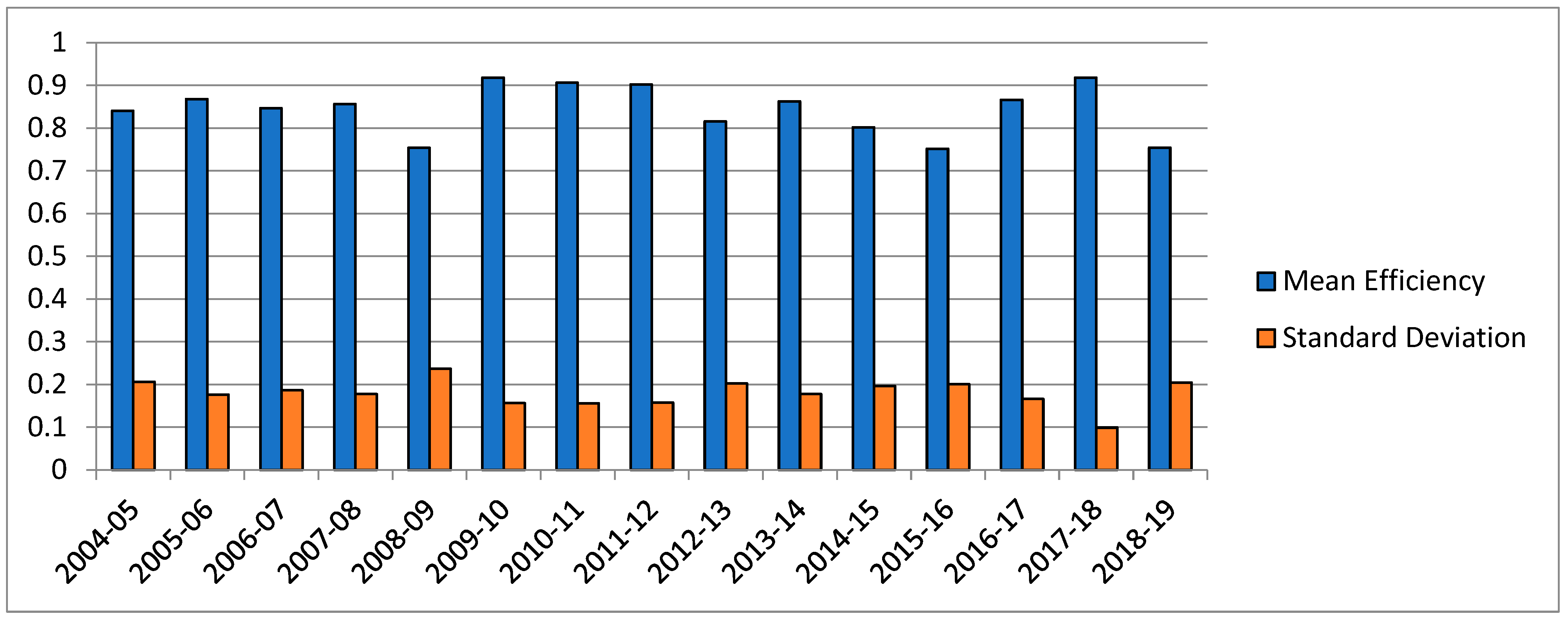
Source: Calculated values.

) for individual efficiency scores). The decline in mean efficiency during 2008–2009 reflects the influence of the global financial crisis, while that of 2015–2016 is reflective of the massive upsurge in the NPA ratio due to a significant erosion in the quality of corporate loan assets. Standard deviation scores are inversely related to the mean efficiency scores. For most of the years, efficiency distribution exhibits negative kurtosis.

Figure 2 graphically presents the trends in mean efficiency and standard deviation for the period under observation.

6.2. Projection Requirements of Inputs and Outputs

Table 5. Mean projection requirements of inputs and outputs (2004–2005 to 2018–2019).

Year	Deposits	Net Worth	NNPA	Advances	Other Income
2004–2005	−3.94	−21.63	−2.27	0.81	17.94
2005–2006	−0.04	−14.39	−4.13	0.051	16.59
2006–2007	−2.21	−23.36	−1.16	0.45	14.87
2007–2008	−0.54	−25.11	−0.34	1.21	8.42
2008–2009	−0.23	−25.27	−36.72	0.19	14.31
2009–2010	−1.3	−6.95	−12.16	0.37	2.34
2010–2011	−1.09	−5.89	−14.88	0.32	5.02
2011–2012	−1.33	−7.17	−15.3	0.68	2.02
2012–2013	0	−14.58	−31.71	1.93	6.9
2013–2014	−0.64	−10.1	−25.22	1	0
2014–2015	−1.11	−14.6	−33.84	1.13	8.6
2015–2016	−1.17	−14.46	−45.36	0.82	22.88
2016–2017	−3.83	−9.12	−19.54	0.05	2.66
2017–2018	−1.64	−4.78	−3.29	1.31	16.87
2018–2019	−9.17	−3.24	−25.54	2.56	71.74
Mean projection requirement	−1.88	−10.26	−18.10	0.86	14.08

Source: Calculated.

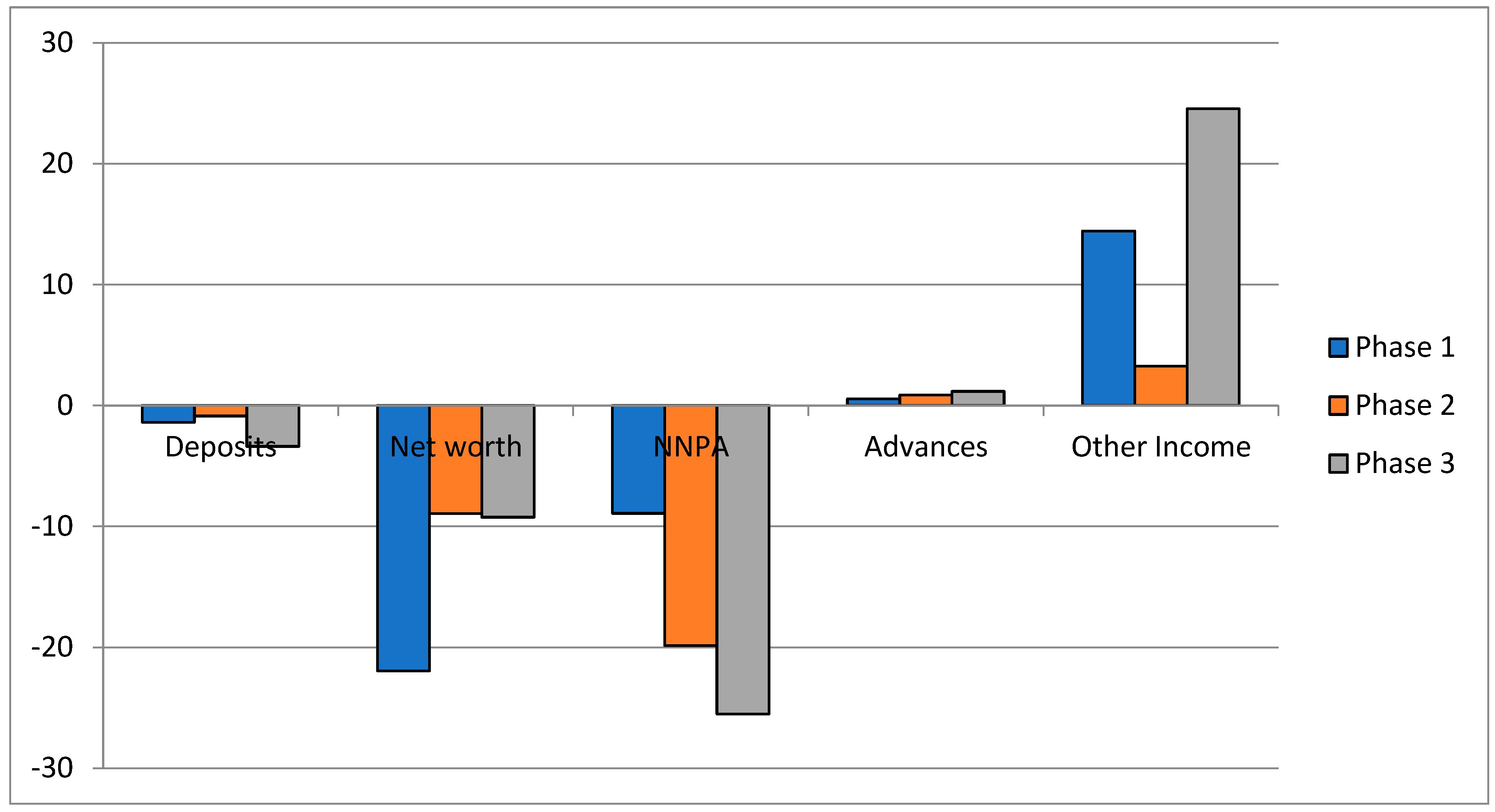
presents the mean percentage changes required in inputs and outputs from their observed levels for the years under observation. Among the two inputs, two good outputs, and one bad output, projection requirement is most important in the case of net non-performing assets (18.1 per cent), followed by other income (14.1 per cent). Table 5 shows that during 2004–2005 to 2008–2009, the average percentage projection (reduction/expansion) requirements of NNPA and other income was 8.92 per cent (reduction) and 14.43 per cent (augmentation), respectively. For the subsequent 5 years, the percentage of required reduction for NNPA jumped to 19.85 while the augmentation requirement for other income declined to 3.26. During the terminal 5 years (2014–2015 through 2018–2019), the per cent projection requirement for NNPA increased further to 25.51 per cent. Similarly, the per cent projection requirement for other income increased to 24.55 per cent.

Figure 3 represents the mean input and output projection requirements for the in-sample public sector banks for three phases: phase 1 (2004–2005 to 2008–2009), phase 2 (2009–2010 to 2013–2014), and phase 3 (2014–2015 to 2018–2019). The figure suggests that, with the exception of the case of net worth, all the inputs and outputs require most projection in the third phase of our in-sample time period.

6.3. Efficiency and NPA Related Performance Across Bank Clusters

For the present study, we classified the in-sample public sector banks into three groups: acquirer banks comprising of five public sector banks (Bank of Baroda, Canara Bank, Indian Bank, Punjab National Bank, and Union Bank of India), which took over eight public sector banks during 2019–2020 and 2020–2021; the acquired bank group including eight banks (Allahabad Bank, Andhra Bank, Corporation Bank, Dena Bank, Oriental Bank of Commerce, Syndicate Bank, United Bank of India, and Vijaya Bank), which were taken over during 2019–2020 and 2020–2021; and the remaining seven banks (State Bank of India, Bank of India, Bank of Maharashtra, Central Bank of India, Indian Overseas Bank, Punjab and Sind Bank, and UCO Bank) which were included in the other bank group. For the entire period, we considered the associates of SBI as part of SBI. Consequently, SBI is included in this other bank group and not in the acquirer bank group.

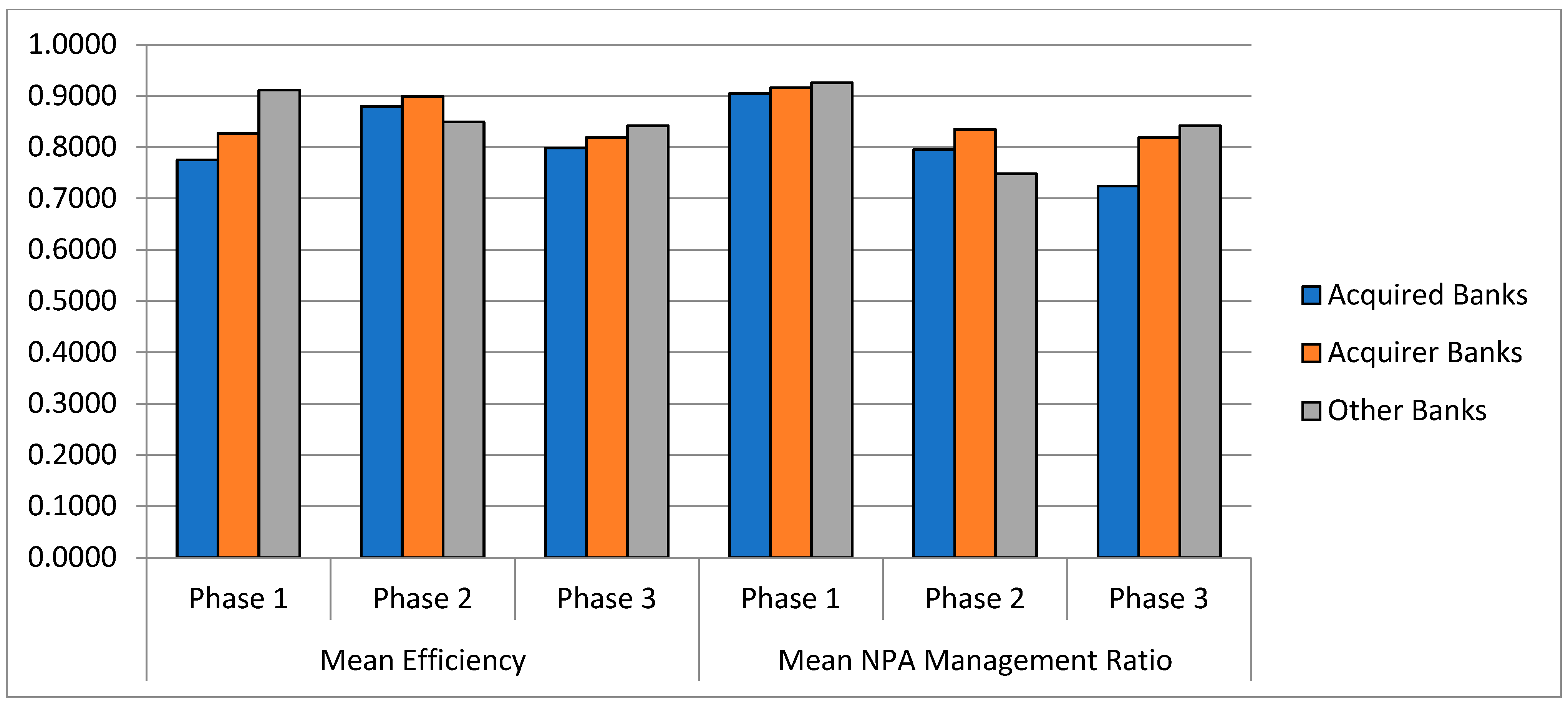
We now consider the performance of the three bank groups for the 15-year period using two metrics: mean efficiency and NPA management ratio. The NPA management ratio is calculated by dividing the projected NPA by the observed level of NPA. We compared the performance for three sub-phases of the in-sample period. Phase 1 includes 2004–2005 through 2008–2009, phase 2 includes mean performance for 2009–2010 through 2013–2014, and phase 3 includes performance for the period 2014–2015 to 2018–2019. The results are presented in

Table 6. Efficiency and NPA management ratio across bank clusters.

Bank Cluster	Mean Efficiency			NPA Management Performance Ratio
	Phase 1	Phase 2	Phase 3	Phase 1	Phase 2	Phase 3
Acquired Banks	0.7748	0.8793	0.7982	0.9042	0.7951	0.7240
Acquirer Banks	0.8268	0.8985	0.8185	0.9154	0.8343	0.8185
Other Banks	0.9109	0.8491	0.8414	0.9254	0.7480	0.8414

Source: Calculated.

and Figure 4. The table clearly shows that for all three phases, the weak and acquired bank groups performed poorly as compared to the acquirer (large) bank group. In the case of the NPA management performance ratio, the difference is much more pronounced in the second and third phases. The comparison of acquirer and other bank groups provides mixed result. In phase 2, the acquirer bank group performed better than the other banks. However, the outcome is just the opposite for the remaining two phases.

6.4. Influence of Contextual Variables

As indicated earlier, the present study seeks to estimate the influence of six contextual variables (return on equity, log of total assets of the banks, capital adequacy ratio, advances to the priority sector, cost of deposits, and regime dummy). Of these, the log of total assets and regime dummy have been used as control variables to control for bank size and the shift in political regime. For this, we used both static and dynamic panel data models. In the static case, we chose the fixed effects approach over the random effects approach based on the Hausman test. In the dynamic case, we applied the Arellano–Bond GMM (generalized method of moments) to estimate the relationship with a 1-period lag in auto regression. Since efficiency scores have both lower and upper bounds, we used the log of efficiency as the dependent variable.

The results of static fixed effects panel data regression and dynamic panel data estimation are presented in

Table 7. Fixed effects regression of efficiency on the contextual variables.

Particulars	Coefficient	Std. Error	t-Ratio	p-Value
Intercept	−1.0990	0.7765	−1.415	0.1732
Return on equity	0.0019	0.0013	1.382	0.1829
LogTA	0.3174	0.1625	1.953	0.0657
Regime Dummy	0.1549	0.0584	2.652	0.0157
Capital Adequacy Ratio	−0.0302	0.0139	−2.177	0.0423
Advances to the priority sector	~0.0000	~0.0000	0.6935	0.4964
Cost of Deposits	−0.0894	0.0253	−3.529	0.0022
Sum squared residual	14.3685
Standard error of regression	0.2290
LSDV R-squared	0.2185

Source: Calculated.

and

Table 8. Dynamic panel data regression of efficiency on the contextual variables.

	Coefficient	Std. Error	t-Ratio	p-Value
LnEff(−1)	0.1703	0.0809	2.107	0.0352
Return on equity	0.0017	0.0016	1.114	0.2654
LogTA	0.5015	0.1258	3.986	<0.0001
Regime Dummy	0.1474	0.0538	2.741	0.0061
Capital Adequacy Ratio	−0.0289	0.0125	−2.316	0.0205
Advances to the priority sector	−9.90079 × 10−7	8.87487 × 10−7	−1.116	0.2646
Cost of Deposits	−0.0809	0.0231	−3.505	0.0005

Source: Calculated.

. In the fixed effects model, the coefficients of four explanatory variables are found to be significant at the 95% level of confidence: log of total asset, regime dummy, capital adequacy ratio, and cost of deposits. Of these, the coefficient of capital adequacy ratio has a negative sign. The coefficients of the remaining three variables (representing bank size, cost of deposit access, and regime shift) are found to be positive. In the dynamic panel data model, the coefficient of the explanatory variables has a similar sign. In addition, one-period lagged log efficiency significantly influences current period log efficiency scores. We tried using higher-order autoregressive processes but the coefficients were insignificant.

We now compare our results with prior studies regarding the influence of profitability, capital adequacy, and cost of deposits. A higher return on equity (ROE) is considered better for a bank, but an extremely high ratio may be indicative of a very low equity capital base or a larger proportion of debt in the capital structure of the company. This, in itself, is a dangerous sign and entails the risk of insolvency. Jelassi and Delhoumi (2021) found that return on equity has insignificant effect on the efficiency of banks. On the other hand, Nouaılı et al. (2015) found a negative relation between efficiency and ROE. Ullah et al. (2023) concluded that in the case of large-sized banks, efficiency is negatively related to ROE, while in the case of small banks, the relation was positive. Thus, mixed results have been found to exist between ROE and bank efficiency. We found that although there is a positive relation between them, it is both extremely low and highly insignificant. This could be due to the fact that higher lending activity does not per se translate into greater profitability and vice versa.

Regarding the relation between capital adequacy ratio and efficiency, in some studies it was found to be positive while in a few others it was found to be negative. In a study of 19 commercial banks of Malaysia from 2005 to 2012, Saha et al. (2015) found a positive relation between CAR and efficiency. Hafez (2018) studied banks in Egypt before and after the financial crisis of 2007–2008. He found a positive relation between CAR and efficiency during the pre-financial crisis period but a negative relation in the post-financial crisis period. We found a significant negative relation between CAR and efficiency. This is not an unusual finding given the imposition of capital adequacy regulation can put a brake on the lending activity of commercial banks.

Finally, we consider the relationship between efficiency and the cost of deposits. Low-cost deposits were found to have a positive impact on the efficiency of banks (Saha et al., 2018; Rehman & Raoof, 2010). We too found a significant negative relation between cost of deposits and efficiency. This is expected since increased borrowing cost acts as a deterrent towards lending. Earlier studies have not found any relation between advances to priority sectors and efficiency (Venugopal, 2024). In the present context, also, the coefficients were not significantly different from zero.

7. Conclusions, Limitations and Future Scope

As indicated earlier, efficient delivery of banking services is of paramount importance for banking services since an inefficient financial institution leads to the transmission of high costs and inefficient operations in the real sector, in addition to leading to adverse macroeconomic consequences. The present study makes an attempt to evaluate and explain public sector bank efficiency in India for the pre-merger phase using a holistic framework that takes into consideration both good and bad outputs of banking activity. Further, our study concentrates on the performance of three categories of public sector banks (acquired banks, acquirer banks, and the remaining banks that were not involved in this consolidation process). For this, the study uses a two-stage approach. In the first stage, we estimated the efficiency performance of the in-sample public sector banks with a special focus on the three categories of banks. In the second stage, we explored the influence of six contextual variables on the estimated efficiency scores.

In the context of banking, the importance of bad loans is of crucial importance. The financial market is a market with asymmetric information, and, with enhanced access to borrower information, the possibility of counterparty default cannot be eliminated. In view of this, we applied an efficiency evaluation framework with undesirable output. The period chosen for the study is interesting for several reasons. First, during the study period, we have witnessed a global financial crisis that led to a prolonged phase of macroeconomic slowdown. Second, the NPA crisis in the in-sample phase was concentrated in the non-priority sector, as the NPA crisis at this time was predominantly connected with unusual credit growth, coupled with macroeconomic slowdown and inadequate monitoring of bank asset quality.

Besides incorporating non-performing assets as an undesirable output, the current study carried out a two-metric performance analysis of the subsequently acquired banks relative to two other bank clusters, which indicates their inherent weaknesses that resulted in their merger with five large public sector banks. This has added to the novelty of the present study. In addition, we applied both static and dynamic panel data models to estimate the influence of profitability (return on equity), capital adequacy, priority sector exposure, and cost of deposits after controlling for bank size and a regime shift. The results indicate that the coefficients of cost of deposits and capital adequacy are negative and statistically significant. On the other hand, the coefficients of return on equity and priority sector exposure are positive but are not significant, in statistical parlance.

Due to the merger of eight weak public sector banks with five large public sector banks, we could not extend our analysis beyond 2018–2019. This is a weakness of our study.

References

- Abidin, Z., Prabantarikso, R. M., Wardhani, R. A., & Endri, E. (2021). Analysis of bank efficiency between conventional banks and regional development banks in Indonesia. The Journal of Asian Finance, Economics and Business, 8(1), 741–750. [Google Scholar]
- Aghayi, N., & Maleki, B. (2016). Efficiency measurement of DMUs with undesirable outputs under uncertainty based on the directional distance function: Application on bank industry. Energy, 112, 376–387. [Google Scholar] [CrossRef]
- Ali, A. I., & Seiford, L. M. (1990). Translation invariance in data envelopment analysis. Operations Research Letters, 9, 403–405. [Google Scholar]
- Allen, F., & Santomero, A. M. (1998). The theory of financial intermediation. Journal of Banking & Finance, 21(11–12), 1461–1485. [Google Scholar]
- Arora, N., Arora, N. G., & Kanwar, K. (2018). Non-performing assets and technical efficiency of Indian banks: A meta-frontier analysis. Benchmarking an International Journal, 25(7), 1–10. [Google Scholar]
- Atkinson, A. B., & Stiglitz, J. E. (1980). Lectures on public economics. Mc-Graw Hill. [Google Scholar]
- Bangarwa, P., & Roy, S. (2021). Application of hybrid approach in banking system: An undesirable operational performance modelling. Global Business Review, 09721509211026789. [Google Scholar] [CrossRef]
- Bangarwa, P., & Roy, S. (2022). Operational performance modelling of indian banks: A data envelopment analysis approach. Paradigm, 26(1), 29–49. [Google Scholar] [CrossRef]
- Bangarwa, P., & Roy, S. (2023). Operational performance model for banks: A dynamic data envelopment approach. Benchmarking: An International Journal, 30(10), 3817–3836. [Google Scholar] [CrossRef]
- Benston, G. (1965). Branch banking and economies of scale. Journal of Finance, 20(2), 312–331. [Google Scholar] [CrossRef]
- Berger, A. N., Hanweck, G. A., & Humphrey, D. B. (1987). Competitive viability in banking: Scale, scope, and product mix economies. Journal of Monetary Economics, 20, 501–520. [Google Scholar] [CrossRef]
- Berger, A. N., & Humphrey, D. (1992). Measurement and efficiency issues in commercial banking. In Z. Griliches (Ed.), Output measurement in the service sectors (pp. 245–300). University of Chicago Press. [Google Scholar]
- Bernanke, B. S. (1983). Nonmonetary effects of the financial crisis in the propagation of the Great Depression. American Economic Review, 73, 257–276. [Google Scholar]
- Bikker, J. A., & Bos, J. W. B. (2008). Bank performance: A theoretical and empirical framework for the analysis of profitability, competition and efficiency (176p). Routledge International Studies in Money and Banking. Routledge. [Google Scholar]
- Boda, M., & Piklová, Z. (2021). Impact of an input-output specification on efficiency scores in data envelopment analysis: A banking case study. RAIRO-Operations Research, 55, S1551–S1583. [Google Scholar]
- Čiković, K. F., KeĆek, D., & Lozić, J. (2023). Does ownership structure affect bank performance in the COVID-19 pandemic period? Evidence from Croatia. Yugoslav Journal of Operations Research, 33(2), 277–292. [Google Scholar] [CrossRef]
- Dar, A. H., Mathur, S. K., & Mishra, S. (2021). The efficiency of Indian banks: A DEA, malmquist and SFA analysis with bad output. Journal of Quantitative Economics, 19, 653–701. [Google Scholar] [CrossRef]
- Diamond, D. (1984). Financial intermediation and delegated monitoring. Review of Economic Studies, 51, 393–414. [Google Scholar] [CrossRef]
- Diamond, D. W., & Dybvig, P. H. (1983). Bank runs, deposit insurance, and liquidity. Journal of Political Economy, 91, 401–419. [Google Scholar]
- Dyckhoff, H., & Allen, K. (2001). Measuring ecological efficiency with data envelopment analysis (DEA). European Journal of Operational Research, 132, 312–325. [Google Scholar]
- Fare, R., & Grosskopf, S. (1995). Environmental decision models with joint outputs. Economics Working Paper Archive. Economic Department, Washington University. [Google Scholar]
- Fare, R., & Grosskopf, S. (2003). Nonparametric productivity analysis with undesirable outputs. American Journal of Agricultural Economics, 85(4), 1070–1074. [Google Scholar]
- Fare, R., & Grosskopf, S. (2004). Modelling undesirable factors in efficiency evaluation: Comment. European Journal of Operational Research, 157, 242–245. [Google Scholar]
- Fare, R., Grosskopf, S., Lovell, C. A. K., & Pasurka, C. A. (1989). Multilateral productivity comparison when some outputs are undesirable: A nonparametric approach. Review of Economics and Statistics, 71, 90–98. [Google Scholar]
- Fare, R., Grosskopf, S., Maryand, N., & Zhongyang, Z. (1994). Productivity growth, technical progress, and efficiency change in industrialized countries. American Economic Review, 84(1), 66–83. [Google Scholar]
- Fare, R., Grosskopf, S., & Tyteca, D. (1996). An activity analysis model of the environmental performance of firms--application to fossil-fuel-fired electric utilities. Ecological Economics, 18(2), 161–175. [Google Scholar]
- Fare, R., Grosskopf, S., & Zaim, O. (2000). An index number approach to measuring environmental performance: An environmental Kuznets curve for OECD countries. In New Zealand Econometrics Study Group Meeting. University of Canterbury. [Google Scholar]
- Fujii, H., Managi, S., & Matousek, R. (2014). Indian bank efficiency and productivity changes with undesirable outputs: A disaggregated approach. Journal of Banking & Finance, 38, 41–50. [Google Scholar]
- Goldsmith, R. W. (1969). Financial structure and development. Yale University Press. [Google Scholar]
- Gomes, E. G., & Lins, M. P. E. (2008). Modelling undesirable outputs with zero sum gains data envelopment analysis models. Journal of the Operational Research Society, 59(5), 616–623. [Google Scholar] [CrossRef]
- Goswami, A., & Gulati, R. (2022). Economic slowdown, NPA crisis and productivity behavior of Indian banks. International Journal of Productivity And Performance Management, 71(4), 1312–1342. [Google Scholar] [CrossRef]
- Greenwood, J., & Jovanovic, B. (1990). Financial development, growth, and the distribution of income. The Journal of Political Economy, 98(5), 1076–1107. [Google Scholar]
- Gurley, J. G., & Shaw, E. S. (1960). Money in a theory of finance. Brookings Institution. [Google Scholar]
- Hafez, M. M. H. (2018). Examining the relationship between efficiency and capital adequacy ratio: Islamic versus conventional banks-an empirical evidence on Egyptian banks. Accounting and Finance Research, 7(2), 232–247. [Google Scholar]
- Hafsal, K., Suvvari, A., & Durai, S. R. S. (2020). Efficiency of Indian banks with non-performing assets: Evidence from two-stage network DEA. Future Business Journal, 6(26), 1–9. [Google Scholar] [CrossRef]
- Hailu, A., & Veeman, T. S. (2001). Nonparametric productivity analysis with undesirable outputs: An application to the Canadian pulp and paper industry. American Journal of Agricultural Economics, 83, 605–616. [Google Scholar]
- Hancock, D. (1985). The financial firm: Production with monetary and nonmonetary goods. Journal of Political Economy, 93(5), 859–880. [Google Scholar]
- Hancock, D. (1991). A theory of production for the financial firm. Kluwer Academic. [Google Scholar]
- Herwadkar, S. S., Goel, S., & Bansal, R. (2022). Privatisation of public sector banks: An alternate perspective (pp. 77–86). RBI Bulletin. [Google Scholar]
- Jelassi, M. M., & Delhoumi, E. (2021). What explains the technical efficiency of banks in Tunisia? Evidence from a two-stage data envelopment analysis. Financial Innovation, 7, 1–26. [Google Scholar] [CrossRef]
- Khati, K. S., & Mukherjee, D. (2021). Productive Efficiency and non-performing assets of Indian Banks in the post-global financial crisis period. South Asia Economic Journal, 22(2), 186–204. [Google Scholar] [CrossRef]
- Korhonen, P., & Luptacik, M. (2003). Eco-efficiency analysis of power plants: An extension of data envelopment analysis. European Journal of Operational Research, 154, 437–446. [Google Scholar] [CrossRef]
- Kumar, A., & Dhingra, S. (2016). Evaluating the efficiency of Indian public sector banks. International Journal of Indian Culture and Business Management, 13(2), 226–242. [Google Scholar] [CrossRef]
- Leland, H. E., & Pyle, D. H. (1977). Informational asymmetries, Financial structure, and Financial intermediation. Journal of Finance, 32, 371–387. [Google Scholar] [CrossRef]
- Liao, C. S. (2018). Deregulation, financial crisis and banks efficiency for Taiwan: Estimation with undesired outputs. Journal of Business, Economics and Finance, 7(1), 17–29. [Google Scholar] [CrossRef]
- Lovell, C. K., Pastor, J. T., & Turner, J. A. (1995). Measuring macroeconomic performance in the OECD: Acomparison of European and non-European countries. European Journal of Operatonal Research, 87(3), 507–518. [Google Scholar] [CrossRef]
- Lowe, P. (1992). The impact of financial intermediaries on resource allocation and economic growth. Research Discussion paper No. 9213. Reserve Bank of Australia. [Google Scholar]
- Mao, X., Guoxi, Z., Fallah, M., & Edalapanah, S. A. (2020). A neutrosophic-based approach in data envelopment analysis with undesirable outputs. Mathematical Problems in Engineering, 5(4), 339–345. [Google Scholar] [CrossRef]
- Mohamadinejad, H., Amirteimoori, A., Kordrostami, S., & Hosseinzadeh, L. F. (2023). A managerial approach in resource allocation models: An application in US and Canadian oil and gas companies. Yugoslav Journal of Operations Research, 33(3), 481–498. [Google Scholar] [CrossRef]
- Nouaılı, M. A., Abaoub, E., & Ochı, A. (2015). The determinants of banking performance in front of financial changes: Case of trade banks in Tunisia. International Journal of Economics and Financial Issues, 5(2), 410–417. [Google Scholar]
- Partovi, E., & Matousek, R. (2019). Bank efficiency and non-performing loans: Evidence from Turkey. Research in International Business and Finance, 48, 287–309. [Google Scholar]
- Puri, J., & Yadav, S. P. (2014). A fuzzy DEA model with undesirable fuzzy outputs and its application to the banking sector in India. Expert Systems with Applications, 41(14), 6419–6432. [Google Scholar] [CrossRef]
- Puri, J., & Yadav, S. P. (2017). Improved DEA models in the presence of undesirable outputs and imprecise data: An application to banking industry in India. International Journal of System Assurance Engineering and Management, 8(2), 1608–1629. [Google Scholar]
- Rawat, S., & Sharma, N. (2023). Impact of non-performing assets over bootstrapped efficiency of banks: Analysis of indian domestic banks. Journal of Business Thought, 14, 35–44. [Google Scholar]
- Rehman, M., & Raoof, A. (2010). Efficiencies of Pakistani banking sector: A comparative study. International Research Journal of Finance and Economies, 46, 110–128. [Google Scholar]
- Reinhard, S., Lovell, C. A. K., & Thijssen, G. J. (2000). Environmental efficiency with multiple environmentally detrimental variables; estimated with SFA and DEA. European Journal of Operational Research, 121(2), 287–303. [Google Scholar]
- Saha, A., Ahmad, N. H., & Dash, U. (2015). Drivers of technical efficiency in Malaysian banking: A new empirical insight. Asian-Pacific Economic Literature, 29(1), 161–173. [Google Scholar] [CrossRef]
- Saha, A., Hock-Eam, L., & Yeok, S. G. (2018). Deciphering drivers of efficiency of bank branches. International Journal of Emerging Markets, 13(2), 391–409. [Google Scholar] [CrossRef]
- Sanati, G., & Bhandari, A. K. (2023). Operational efficiency in the presence of undesirable byproducts: An analysis of Indian banking sector under traditional and market based banking framework. NIBM Working Paper Series WP24/May. National Institute of Bank Management. [Google Scholar]
- Scheel, H. (2001). Undesirable outputs in efficiency evaluations. European Journal of Operational Research, 132, 400–410. [Google Scholar] [CrossRef]
- Sealey, C. W., Jr., & Lindley, J. T. (1977). Inputs, outputs, and a theory of production and cost at depository financial institutions. The Journal of Finance, 32(4), 1251–1266. [Google Scholar]
- Seiford, L. M., & Zhu, J. (2002). Modeling undesirable factors in efficiency evaluation. European Journal of Operational Research, 142, 16–20. [Google Scholar]
- Shi, Y., Yu, A., Higgins, H. N., & Zhu, J. (2021). Shared and unsplittable performance links in network DEA. Annals of Operations Research, 303, 507–528. [Google Scholar] [CrossRef]
- Stiglitz, J. E. (1989). Markets, market failures, and development. The American Economic Review, 79(2), 197–203. [Google Scholar]
- Subramanyam, T., Zalki, M., Satish Kumar, V., & Amalanathan, S. (2023). Efficiency of Indian banks with non-performing assets as undesirable outputs. AIP Conference Proceedings, 2649, 030063. [Google Scholar] [CrossRef]
- Tanwar, J., Seth, H., Vaish, A. K., & Rao, N. V. M. (2020). Revisiting the efficiency of indian banking sector: An analysis of comparative models through data envelopment analysis. Indian Journal of Finance and Banking, 4(1), 92–108. [Google Scholar]
- Tone, K. (2004, June 23–25). Dealing with undesirable outputs in DEA: A Slacks-Based Measure (SBM) approach. North American Productivity Workshop 2004 (pp. 44–45), Toronto, ON, Canada. [Google Scholar]
- Ullah, S., Majeed, A., & Popp, J. (2023). Determinants of bank’s efficiency in an emerging economy: A data envelopment analysis approach. PLoS ONE, 18(3), e0281663. [Google Scholar] [CrossRef]
- Venugopal, S. K. (2024). Loan portfolio management and bank efficiency: A comparative analysis of public, old private, and new private sector banks in India. Economies, 12(4), 81. [Google Scholar] [CrossRef]
- Wijesiri, M., Martínez-Campillo, A., & Wanke, P. (2019). Is there a trade-off between social and financial performance of public commercial banks in India? A multi-activity DEA model with shared inputs and undesirable outputs. Review of Managerial Science, 13(2), 417–442. [Google Scholar]
- Yaisawarng, S., & Klein, J. D. (1994). The effects of sulfur dioxide controls on productivity change in the U.S. electric power industry. Review of Economics & Statistics, 76, 447–460. [Google Scholar]
- Zhou, L., & Zhu, S. (2016). Research on the efficiency of Chinese commercial banks based on undesirable output and super-SBM DEA model. Journal of Mathematical Finance, 7, 102–120. [Google Scholar]
- Zofio, J. L., & Prieto, A. M. (2001). Environmental efficiency and regulatory standards: The case of CO2 emissions from OECD industries. Resource and Energy Economics, 23, 63–83. [Google Scholar] [CrossRef]