Article

Sample Path Generation of the Stochastic Volatility CGMY Process and Its Application to Path-Dependent Option Pricing

College of Business, Stony Brook University, Stony Brook, NY 11794, USA
J. Risk Financial Manag. 2021, 14(2), 77; https://doi.org/10.3390/jrfm14020077
Submission received: 25 January 2021 / Revised: 6 February 2021 / Accepted: 12 February 2021 / Published: 15 February 2021
(This article belongs to the Special Issue Mathematical and Empirical Finance)

Abstract

:
This paper proposes the sample path generation method for the stochastic volatility version of the CGMY process. We present the Monte-Carlo method for European and American option pricing with the sample path generation and calibrate model parameters to the American style S&P 100 index options market, using the least square regression method. Moreover, we discuss path-dependent options, such as Asian and Barrier options.
JEL Classification:
C15; C22; C60; G13

1. Introduction

Lévy process models have played a role as the standard framework for option pricing, since these models allow for stochastic volatility and the volatility smile effect observed for the Black Scholes model (Black and Scholes (1973)). For instance, Hurst et al. (1999) applied an α -stable process, Carr et al. (2002) used the Carr, Geman, Madan, and Yor (CGMY) process, which is a subclass of the tempered stable process (Rosiński 2007), and Bianchi et al. (2010) presented the tempered, infinitely divisible model. Moreover, Lévy process models with time-varying volatility have been used for option pricing in discrete time models, since empirical studies show that Brownian motion is often rejected (see Rachev and Mittnik (2000), Kim et al. (2010), Kim et al. (2011)). Carr et al. (2003) defined the class of continuous time stochastic volatility models on Lévy processes (SVLP) using the time-changed Lévy process. The SVLP model has been successfully applied in European option pricing, but the absence of an efficient sample path generation method makes the SVLP model hard to apply to path-dependent options, such as American, Barrier, or Asian options.
This paper proposes a sample path generation method for the stochastic volatility version, CGMYSV, of the CGMY process, which is a subclass of the SVLP model. The method is constructed by an approximation to the series representation of the CGMY process with the time-varying scale parameter. The series representations for the tempered stable and tempered infinitely divisible distributions are discussed in Rosiński (2007) and Bianchi et al. (2010), and they are applied to the Monte-Carlo simulation (MCS) of the CGMY market model with a GARCH volatility in Kim et al. (2010). We note that the CGMYSV model is a continuous-time model, different from the GARCH model with CGMY innovations. We develop an algorithm for CGMYSV sample path generation, and apply it to MCS. The algorithm is used to price European and American options and to calibrate the risk-neutral parameters to the S&P 500 index option (European style) data and S&P 100 option (American style) data. We use the least square regression method by Longstaff and Schwartz (2001) for pricing American options with MCS. We verify empirically that the new sample path generation method performs well in pricing American options. We also apply the algorithm to the pricing of Asian and Barrier options with MCS.
This paper is organized as follows. A continuous time stochastic volatility model and the CGMY process with the series representation are presented briefly in Section 2. The sample path generation method based on the series representation is constructed in Section 3. In Section 4, we calibrate the CGMYSV model to S&P 500 index option and S&P 100 index option data, and discuss Asian and Barrier option prices. Conclusions are presented in Section 5.

2. Preliminary

To construct the CGMYSV model, we take the CGMY process and employ the Cox-Ingersoll-Ross (CIR) process (Cox et al. 1985) for the stochastic volatility, which, as in Heston (1993), enhances the Black Scholes model. In this section, we briefly discuss the CIR model and the CGMY process. The CGMYSV model is presented in the next section.

2.1. CIR Model

The CIR model is given by
d v t = κ ( η v t ) d t + ζ v t d W t and v 0 > 0 ,
for κ , η , ζ > 0 and Brownian motion { W t } t 0 . Let F t v be a smallest σ -algebra generated by the process { v s } 0 s t , then v t + Δ t | F t v = d ξ / ( 2 c ) where c = 2 κ ( 1 e κ Δ t ) ζ 2 and the random variable ξ is a noncentral χ 2 -distributed random variable with 4 κ η / ζ 2 degrees of freedom and noncentrality parameter 2 c v t e κ Δ t .
Let V t = 0 t v s d s . Then, the joint distribution of v t , V t has the characteristic function (Ch.F) Φ t ( a , b , x ) = E exp ( a V t + i b v t ) | v 0 = x given by (Proposition 6.2.5 in Lamberton and Lapeyre (1996)):
Φ t ( a , b , x ) = A ( t , a , b ) exp B ( t , a , b ) x ,
with
A ( t , a , b ) = exp κ 2 η t ζ 2 cosh γ t 2 + κ i b ζ 2 γ sinh γ t 2 2 κ η / ζ 2 B ( t , a , b ) = i b γ cosh γ t 2 κ sinh γ t 2 + 2 i a sinh γ t 2 γ cosh γ t 2 + κ i b ζ 2 sinh γ t 2 γ = κ 2 2 ζ 2 i a .

2.2. CGMY Process

Let α ( 0 , 2 ) , C , λ + , λ > 0 , and μ R . Suppose X is an infinitely divisible random variable with Ch.F
ϕ X ( u ) = E [ e i u X ] = ϕ C G M Y ( u ; α , C , λ + , λ , μ ) = exp ( μ C Γ ( 1 α ) ( λ + α 1 λ α 1 ) ) i u C Γ ( α ) ( λ + i u ) α λ + α + ( λ + i u ) α λ α .
We refer to X as a CGMY-distributed random variable with parameters ( α , C, λ + , λ , μ ) 1, which we denote as X CGMY ( α , C, λ + , λ , μ ) .
Let C = ( Γ ( 2 α ) ( λ + α 2 + λ α 2 ) ) 1 and μ = 0 . Then, a CGMY random variable Z CGMY ( α , C, λ + , λ , μ ) has zero mean ( E [ Z ] = 0 ) and unit variance ( var ( Z ) = 1 ). In this case, we say that Z is standard CGMY-distributed, and denote this by Z stdCGMY ( α , λ + , λ ) . Moreover, the Ch.F of Z is given by
ϕ stdCGMY ( u ; α , λ + , λ ) = ϕ Z ( u ) = E [ e i u Z ] = exp λ + α 1 λ α 1 ( α 1 ) ( λ + α 2 + λ α 2 ) i u + ( λ + i u ) α λ + α + ( λ + i u ) α λ α α ( α 1 ) ( λ + α 2 + λ α 2 ) .
Since the CGMY distribution is non-Gaussian and infinitely divisible, it generates a pure jump Lévy process { X t } t 0 , such that X 1 CGMY ( α , C, λ + , λ , μ ) . In this case, we say that { X t } t 0 is a CGMY process with parameters ( α , C, λ + , λ , μ ) . The Ch.F of X t is equal to
ϕ X t ( u ) = exp ( t log ( ϕ CGMY ( u ; α , C , λ + , λ , μ ) ) ) .
Following the same argument, a pure jump Lévy process { Z t } t 0 is generated by the standard CGMY distribution, such that Z 1 stdCGMY ( α , λ + , λ ) is referred to as the standard CGMY process with parameters ( α , λ + , λ ) . The CGMY and standard CGMY processes are characterized by their Lévy symbols
ψ CGMY ( u ; α , C , λ + , λ , μ ) = log ϕ CGMY ( u ; α , C , λ + , λ , μ ) ,
and
ψ stdCGMY ( u ; α , λ + , λ ) = log ϕ stdCGMY ( u ; α , λ + , λ ) ,
respectively.

2.3. Series Representation of the CGMY Process

Rosiński (2007) introduced the series representation form for the tempered stable random variable and process. The series representation form has been used for CGMY sample path generation by Kim et al. (2010) and Rachev et al. (2011). Assume that X CGMY ( α , C, λ + , λ , 0 ) . Let { U j } j = 1 , 2 , be an independent and identically distributed (i.i.d.) sequence of uniform random variables on ( 0 , 1 ) . Let { E j } j = 1 , 2 , be i.i.d. sequences of exponential random variables with parameters 1, and let { Γ j } j = 1 , 2 , be a Poisson point process with parameter 1. Let { V j } j = 1 , 2 , be an i.i.d. sequence of random variables in { λ + , λ } with P ( V j = λ + ) = P ( V j = λ ) = 1 / 2 . Suppose that { U j } j = 1 , 2 , , { V j } j = 1 , 2 , , { E j } j = 1 , 2 , , and { Γ j } j = 1 , 2 , are independent. Then, X is represented by the following series form:
X = j = 1 α Γ j 2 C 1 / α E j U j 1 / α | V j | 1 V j | V j | + b ,
where b = C Γ ( 1 α ) λ + α 1 λ α 1 . Let { τ j } j = 1 , 2 , be an i.i.d. sequence of uniform random variables on ( 0 , T ) independent of { U j } j = 1 , 2 , , { V j } j = 1 , 2 , , { E j } j = 1 , 2 , , and { Γ j } j = 1 , 2 , . Suppose
X t = j = 1 α Γ j 2 C T 1 / α E j U j 1 / α | V j | 1 V j | V j | 1 τ j t + t b T , t [ 0 , T ] ,
where b T = C Γ ( 1 α ) λ + α 1 λ α 1 . Then, the process { X t } t [ 0 , T ] is the CGMY process with parameters ( α , C, λ + , λ , 0 ) for the time horizon T > 0 .

3. Stochastic Volatility Version of the CGMY Process

Suppose { Z t } t 0 is the standard CGMY process with parameters ( α , λ + , λ ) and { v t } is the stochastic volatility process given by the CIR model in (1). We define a process { L t } t 0 by
L t = Z V t + ρ v t ,
where V t = 0 t v s d s , and { Z t } t 0 is independent of the process { v t } t 0 . The process { L t } t 0 is referred to as the stochastic volatility version of the CGMY process, or simply the CGMYSV process2, with parameters ( α , λ + , λ , κ , η , ζ , ρ , v 0 ) . By (2), the characteristic function of L t is
ϕ L t ( u ) = Φ t ( i ψ stdCGMY ( u ; α , λ + , λ ) , ρ u , v 0 ) ,
where ψ stdCGMY ( u ; α , λ + , λ ) is the Lévy symbol of { Z t } t 0 defined in (4).

3.1. Discrete Time Approximation of the CGMYSV Process

Suppose that we have: a CIR process { v t } t 0 with parameters κ , η , and ζ , as defined in (1); V t = 0 t v s d s for t > 0 ; and suppose that { F t v } t 0 is natural filtration generated by { v t } t 0 . Let P = { 0 = t 0 < t 1 < < t m < < M = T } be the time partition, Δ t m = t m t m 1 for m { 1 , 2 , , M } , and let | | P | | = max { Δ t m | m = 1 , 2 , , M } . Suppose that { v t m } t m P and { L t m } t m P are discrete sub-sequences of the CIR process and the CGMYSV process, respectively. Let Δ L t m = L t m L t m 1 , Δ V t m = V t m V t m 1 , and Δ v t m = v t m v t m 1 . Then we have
Δ L t m | F t m 1 v = d ( Z V t m V t m 1 ) | F t m 1 v + ρ ( v t m v t m 1 ) | F t m 1 v = Z Δ V t m | F t m 1 v + ρ ( Δ v t m | F t m 1 v ) ,
where
Z Δ V t m | F t m 1 v CGMY α , C ( Δ V t m | F t m 1 v ) , λ + , λ , 0 ,
and C = Γ ( 2 α ) ( λ + α 2 + λ α 2 ) 1 . Since we approximate
Δ V t m | F t m 1 v = t m 1 t m v t d t v t m 1 Δ t m ,
we have
Z Δ V t m | F t m 1 v Z v t m 1 Δ t m | F t m 1 v CGMY α , C v t m 1 Δ t m , λ + , λ , 0 .
Suppose { Y t m } t m P is a process defined by
Y t m = Y t m 1 + Z v t m 1 Δ t m | F t m 1 v , m = 1 , 2 , , M ,
with Y 0 = 0 , then Y t m Z V t m | F t m 1 v and { Y t m } t m P is an approximation of the process Z V t m | F t m 1 v t m P .
By the series representation, we have
Z v t m 1 Δ t m | F t m 1 v = d j = 1 α Γ j 2 c m Δ t m 1 / α E j U j 1 / α | V j | 1 V j | V j | + b m Δ t m ,
where b m = c m Γ ( 1 α ) λ + α 1 λ α 1 , c m = v t m 1 C , and { U j } j = 1 , 2 , , { V j } j = 1 , 2 , , { E j } j = 1 , 2 , , and { Γ j } j = 1 , 2 , are given in Section 2.3. Following the same argument as the series representation of the CGMY process presented in Section 2.3, we can define a series representation of Y t m as follows:
Y t m = j = 1 α Γ j 2 c ( τ j ) T 1 / α E j U j 1 / α | V j | 1 V j | V j | 1 τ j t m + k = 1 m b k Δ t k ,
where
b k = v t k 1 λ + α 1 λ α 1 ( 1 α ) ( λ + α 2 + λ α 2 ) ,
c ( τ j ) = C m = 1 M v t m 1 1 t m 1 < τ j t m ,
and { τ j } j = 1 , 2 , is an i.i.d. sequence of uniform random variables on ( 0 , T ) independent of { U j } j = 1 , 2 , , { V j } j = 1 , 2 , , { E j } j = 1 , 2 , , and { Γ j } j = 1 , 2 , .
Since we have
L t m = k = 1 m Δ L t k | F t k 1 v k = 1 m Z v t k 1 Δ t k | F t k 1 v + ρ Δ v t k | F t k 1 v = k = 1 m Y t k Y t k 1 + ρ Δ v t k | F t k 1 v by ( 7 ) ,
we obtain
L t m Y t m + ρ v t m ,
as | | P | | 0 . Let
L ^ t m = Y t m + ρ v t m , t m P \ { 0 }
and L ^ 0 = L 0 . Then, the discrete process { L ^ t m } t m P is an approximation of { L t m } t m P . In this case, the process { L ^ t m } t m P is referred to as the discrete time approximation of the CGMYSV process, or simply the C G M Y S V ^ process. Combining Equations (8) and (9), we can generate a C G M Y S V ^ sample path, as illustrated in Algorithm 1.

3.2. Simulation of the CGMYSV Process

In order to verify the performance of Algorithm 1, we generate a set of example sample paths of the C G M Y S V ^ process { L ^ t m } t m P and compare it to the distribution of the CGMYSV process { L t } t 0 with parameters α = 0.52 , λ + = 25.46 , λ = 4.604 , κ = 1.003 , η = 0.0711 , ζ = 0.3443 , v 0 = 0.0064 , and ρ = 2.0280 . We set M = 100 , J = 1024 , N = 10 , 000 , and Δ t = 1 / 252 , which is the annual fraction represented by one trading day. For example, 20 sample paths are presented in the first plate of Figure 1. The second plate of the figure is for 20 sample paths of the CIR process. For the goodness-of-fit test for the generated path, we perform the Kolmogorov–Smirnov (KS) test. We compare the distribution L ^ 10 Δ t to the distribution of L 10 Δ t . That is, we compare the distribution of 10-day simulated random numbers { L n , 10 | n = 1 , 2 , , N } with the distribution of L 10 Δ t . The cumulative distribution function of L 10 Δ t can be obtained by the Ch.F of the CGMYSV using the inverse Fourier-Transform method (See Rachev et al. (2011) for more details). Table 1 presents the results of the KS test. The p-value for the KS statistic for 10 days is 70.29%, which is not rejected at the 5% significance level. Using the same argument, we perform KS tests for 25 days, 50 days, and 100 days of simulated random numbers. They are not rejected at the 5% significance level, either. We graphically compare the empirical probability density function (pdf) of the simulated sample path and the CGMYSV pdfs for those four cases. We draw empirical pdfs using gray bar charts and draw solid lines for CGMYSV pdfs in four plates in Figure 2.
Algorithm 1: CGMYSV sample path generation.
Jrfm 14 00077 i001

4. The CGMYSV Option Pricing Model

In this section, we discuss the option pricing model using the CGMYSV model. We define the model and calibrate its parameters using the European style, S&P 500 index option (SPX option) data, and the American style S&P 100 index option (OEX option) data.
Let r and q be the risk-free rate of return and the continuous dividend rate of a given underlying asset, respectively. The risk-neutral price process { S t } t 0 of the underlying asset is assumed to be
S t = S 0 exp ( ( r q ) t + L t ) E exp ( L t ) ,
where { L t } t 0 is the CGMYSV process with parameters ( α , λ + , λ , κ , η , ζ , ρ , v 0 ) . By (6), we also have
S t = S 0 exp ( ( r q ) t + L t ) Φ t ( i log ϕ s t d C T S ( i ; α , λ + , λ ) , ρ i , v 0 ) .

4.1. Calibration to European Options

For the risk-neutral price process { S t } t 0 defined by (10), the European call and put prices, with strike price K and time to maturity T, are given by C ( K , T ) = e r T E [ ( S t K ) + ] and C ( K , T ) = e r T E [ ( K S t ) + ] , respectively. Using the fast Fourier transform (FFT) method of Carr and Madan (1999), we can calculate European call/put prices numerically. We calibrate the CGMYSV parameters ( α , λ + , λ , κ , η , ζ , ρ , v 0 ) using the SPX option prices for 11 September 2017. We observed 247 call prices and 289 put prices on that day. The S&P 500 price, S 0 , risk-free rate of return, r, and continuous dividend rate, q, on that day were S 0 = 2488.11 , r = 1.213 % , and q = 1.884 % . The calibration results for SPX calls and puts are provided in Table 2. 
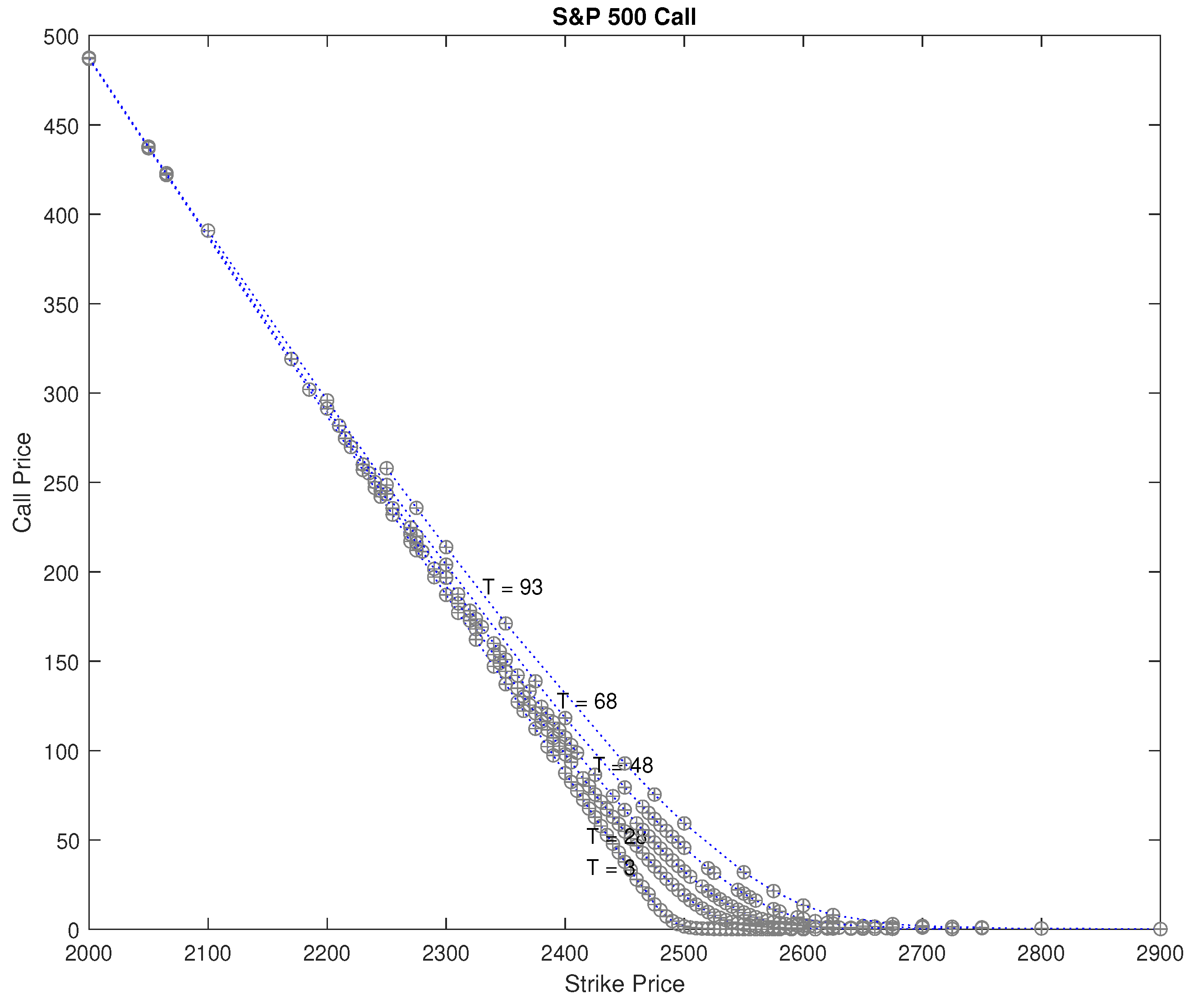
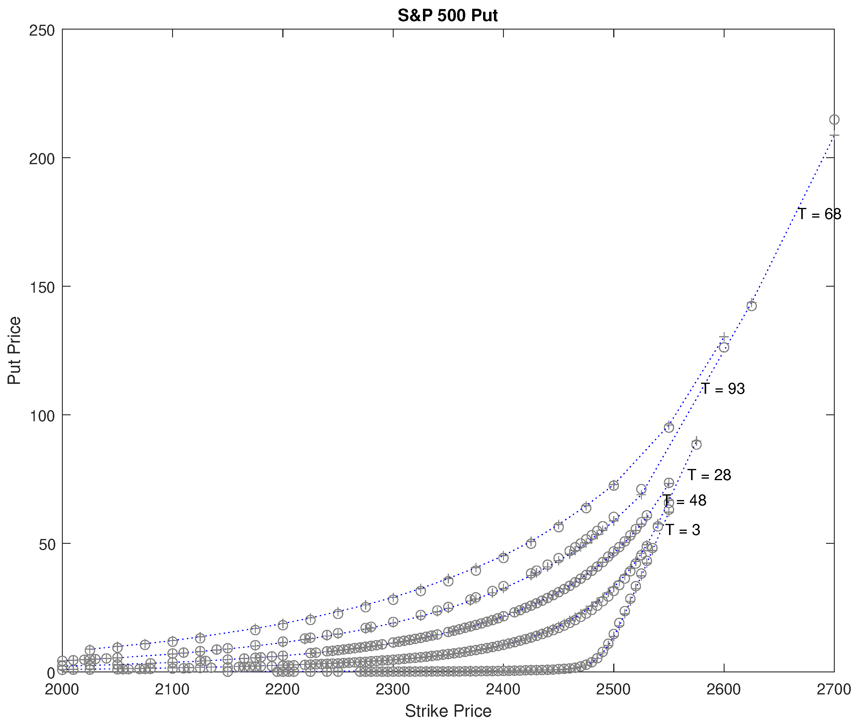
Figure 3 shows observed SPX call and put prices, and calibrated CGMYSV prices using the FFT.
We recalculate the European call and put prices using the MCS method with the calibrated parameters from Table 2. The sample paths of the MCS method are generated by Algorithm 1. We used 10,000 sample paths. To compare the MCS method with the FFT method, we use the four error estimators: the average absolute error (AAE), the average absolute error as a percentage of the mean price (APE), the average relative percentage error (ARPE), and the root mean square error (RMSE) (see Schoutens (2003)).3 The measured values for these error estimators, for the FFT method and the MCS method, are in Table 3. In all cases but one, for both the call and put cases, the MCS method has larger error values than the FFT method. This is not surprising because we calibrated the parameters using the FFT method. However, while larger, the error values for the MCS method are similar to those of the FFT method. That means the sample path generation with Algorithm 1 performs well, and prices by the MCS perform similarly to those for the FFT method.
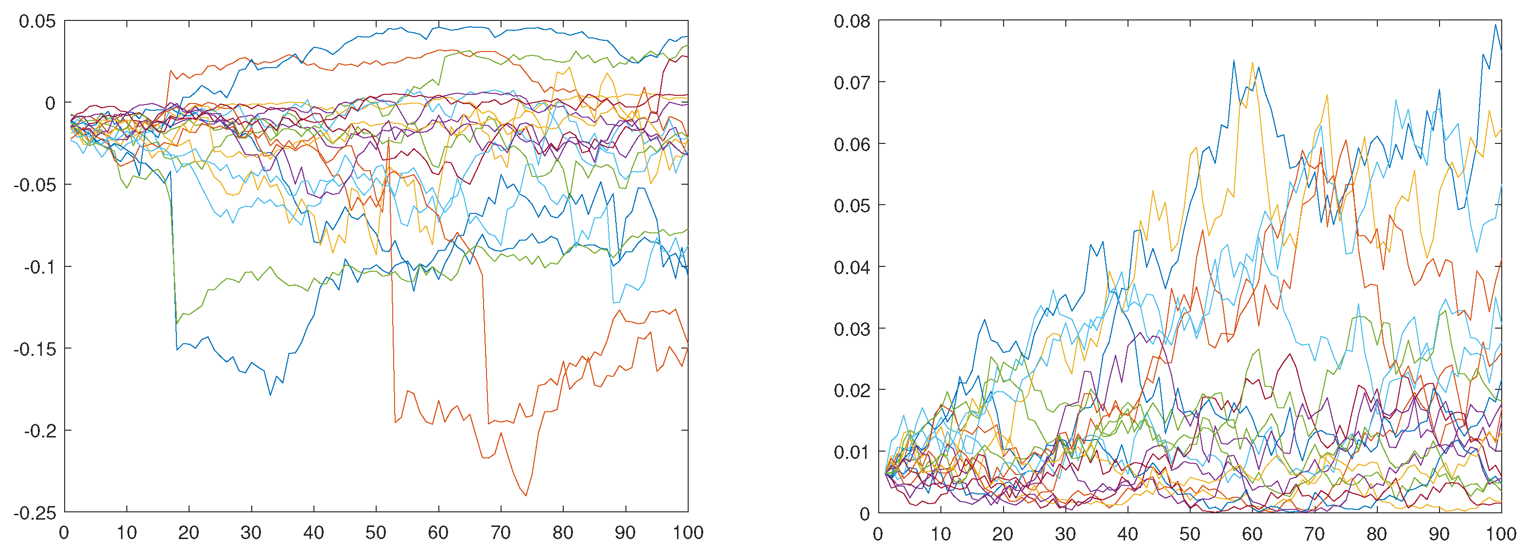
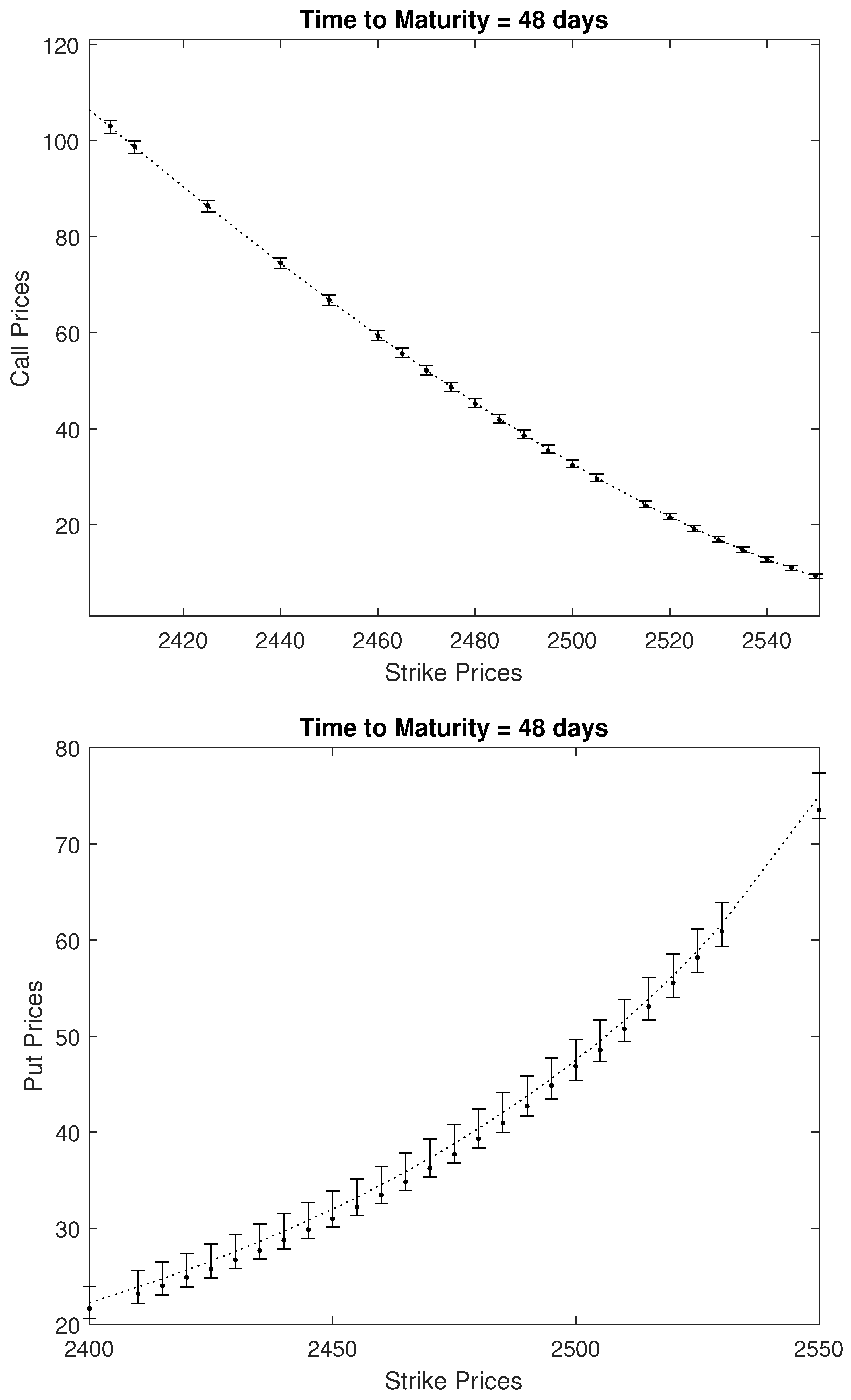
For the option prices computed with the MCS method, we obtain standard error estimates for each 247 call and 289 put option. (Not presented due to page limitations.) Instead, in Figure 4, we plot MCS prices and the 95% confidence intervals for case 2400 < K < 2600 , and time to maturity T = 48 d a y s .
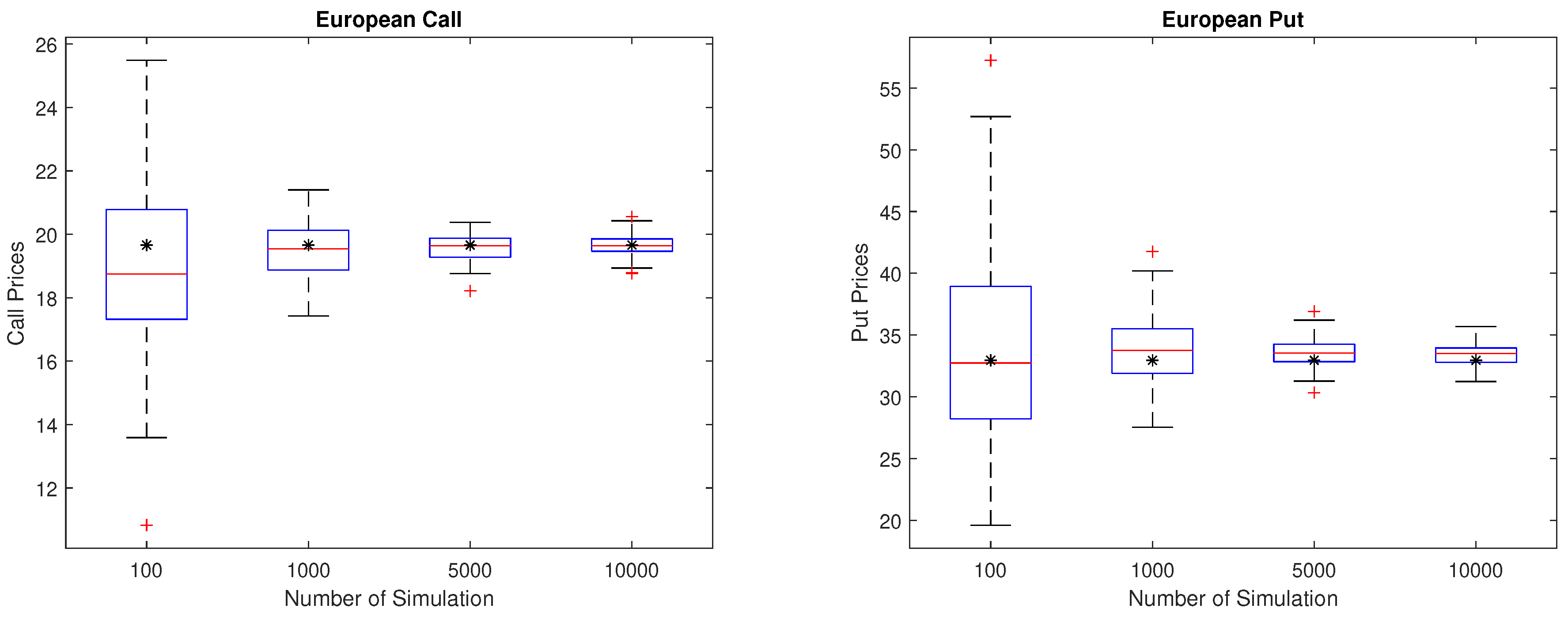
Finally, we perform the bootstrapping. We select an at-the-money call, and an at-the-money put of K = 2500 and T = 28 d a y s as examples, and calculate call and put prices with the MCS parameters in Table 2. Table 4 shows that the MCS prices and their standard errors for 100, 1000, 5000, and 10,000 sample paths. We repeat this process 100 times. Boxplot summaries of the statistics for the resulting call and put prices for each number of sample paths are presented in Figure 5. We also show (by the symbol ’*’) the call/put prices computed using the FFT method. We observe that, as the number of sample paths increases, the interquartile distance of MCS prices narrows to that of the FFT price and dispersions are reduced.

4.2. Calibration to American Options

In Section 4.1, we have seen that the sample path generation method using the series representation works for the MCS method for European option pricing. In this section, we discuss the American option pricing with the same sample path generation method. We use the least squares regression method (LSM) of Longstaff and Schwartz (2001) for American option pricing with the MCS method. When we perform the regression for the expected value of an option, we consider S t , S t 2 , σ t , σ t 2 , and σ t S t as independent variables, following the idea in Chapter 15 of Rachev et al. (2011).
For empirical illustration, we use market prices of the American style OEX option. We calibrate the parameters of the CGMYSV model with fixed seed numbers for each random number generation. That is, we fix the seed value for the chi-square random number generator in the CIR process, and generate uniform and exponential random numbers U j , U j , E j , E j , and τ j with the predefined seed values. Then we set the model parameters, generate C G M Y S V ^ sample paths using Algorithm 1 with the fixed seed number and the fixed random number sets, and then calculate American option price using LSM. We find the optimal model parameters to minimize RMSE. As a benchmark, we calibrate the parameters of the CGMY option pricing model (See Carr et al. (2002)) with the OEX option price data using LSM, with sample paths generated by the series representation explained in Section 2.3.
The calibration results are presented in Table 5. We calibrate the CGMY and the CGMYSV model parameters for 12 Wednesdays in 2015 and 2016. Values for the four error estimators, AAE, APE, ARPE, and RMSE, are provided in Table 6. As smaller error values imply better calibration performance, smaller errors are written in bold letters. Table 6 shows that the CGMYSV calibration performs better than the CGMY calibration, except for 10 February 2016, and 10 June 2015. On 9 March 2016, AAE and APE values for the CGMY model are less than those of CGMYSV, but ARPE and RMSE values for CGMY are larger than those for CGMYSV. The ARPE value for CGMY is smaller than that of CGMYSV on 10 November 2015, but the other three error values for CGMY are larger than that for CGMYSV. Therefore, we can conclude that, in this investigation, the CGMYSV option pricing model typically performs better than the CGMY option pricing model, except in a few cases. Hence, the LSM with Algorithm 1 works well for the American option calibration.
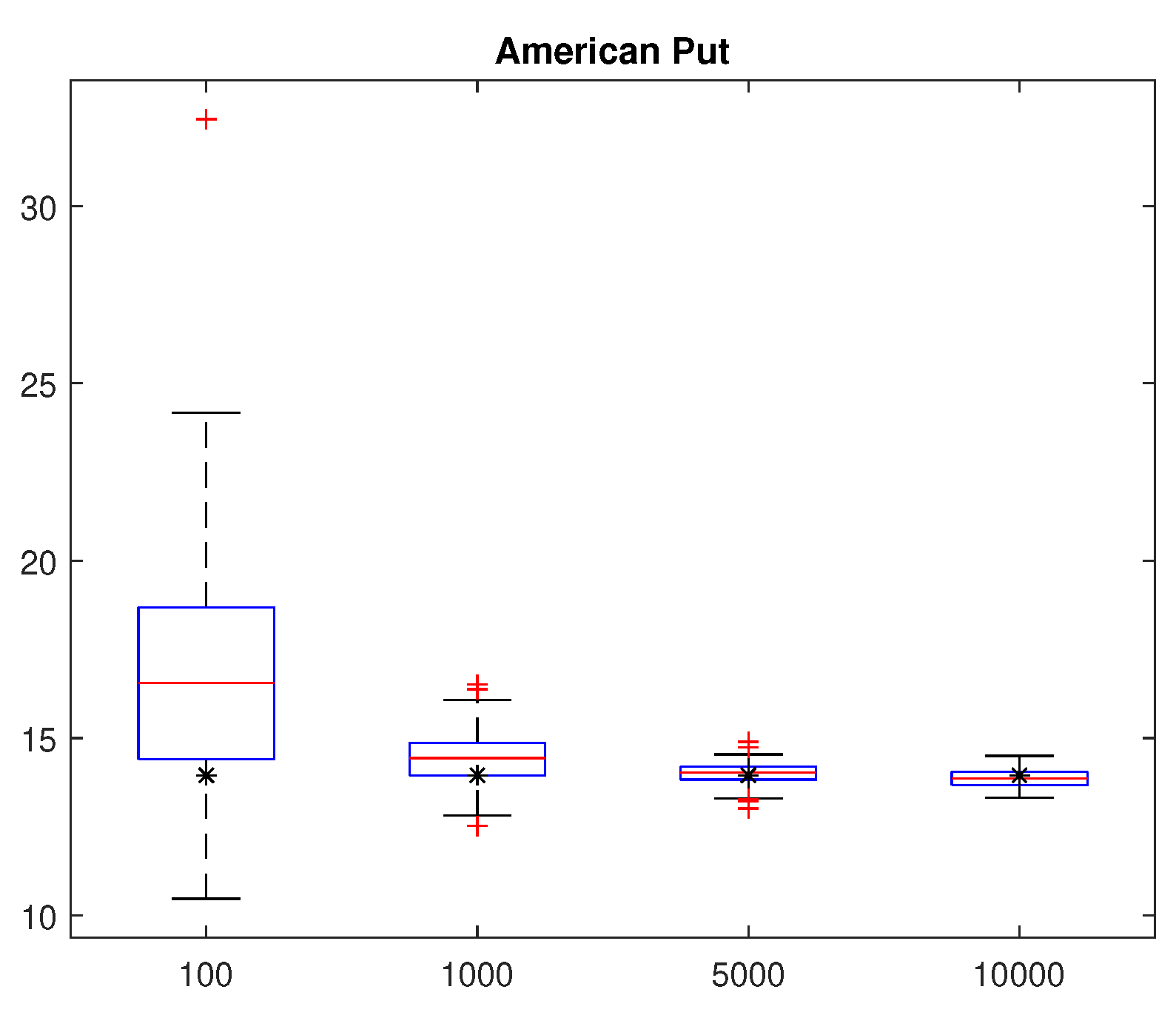
Finally, we perform bootstrapping. We selected the at-the-money, 6 April 2016 put option with strike price K = 910 and T = 31 days to maturity. Put prices were obtained by LSM using the parameters calibrated for that day in Table 5. On that day, the underlying S&P 100 index price was 918.21, and the market put price was 13.95. Table 7 shows the LSM prices and their standard errors for simulation using 100, 1000, 5000, and 10,000 sample paths. The LSM prices approach the market price, and the standard error decreases as the number of sample paths increases. We repeated these simulations 100 times, and present numerical summaries for the statistics for those 100 prices in Table 8. As the number of sample paths increases, means and medians approach the market put price, while the standard deviations and ranges are decreased. We present boxplot summaries in Figure 6 for those 100 prices. Market put prices are also represented (’*’ symbols) with the boxplots. We observe that the interquartile distance of LSM prices narrows to that of the market price, and dispersions are reduced as the number of sample paths increase.
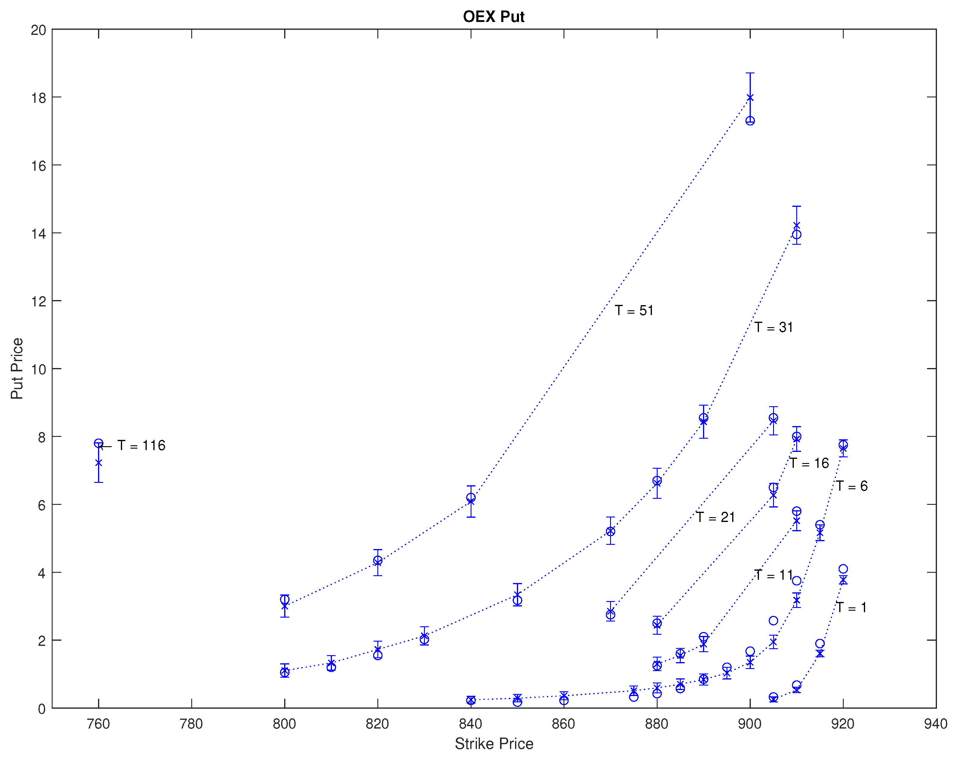
Figure 7 provides a graphical illustration of the calibration for 6 April 2016. Calibrated CGMYSV prices are drawn by "×", the market observed prices are drawn by "∘", and the 95% confidence intervals are marked by a "I" shape. The days to maturities T are written on the plate.

4.3. Asian and Barrier Options

The sample path generation method for the CGMYSV model can also be used for Asian and Barrier option pricing. In this section, we briefly show examples of Asian and Barrier option pricing using the MCS, with sample paths generated by Algorithm 1. We generated 10,000 sample paths of the CGMYSV model with parameters α = 0.52 , λ + = 25.46 , λ = 4.604 , κ = 1.003 , η = 0.0711 , ζ = 0.3443 , v 0 = 0.0064 , and ρ = 2.0280 . Then, we generated the underlying price process { S t } t 0 using (10), where S 0 = 2 , 488 , r = 0.0121 , and d = 0.0188 .
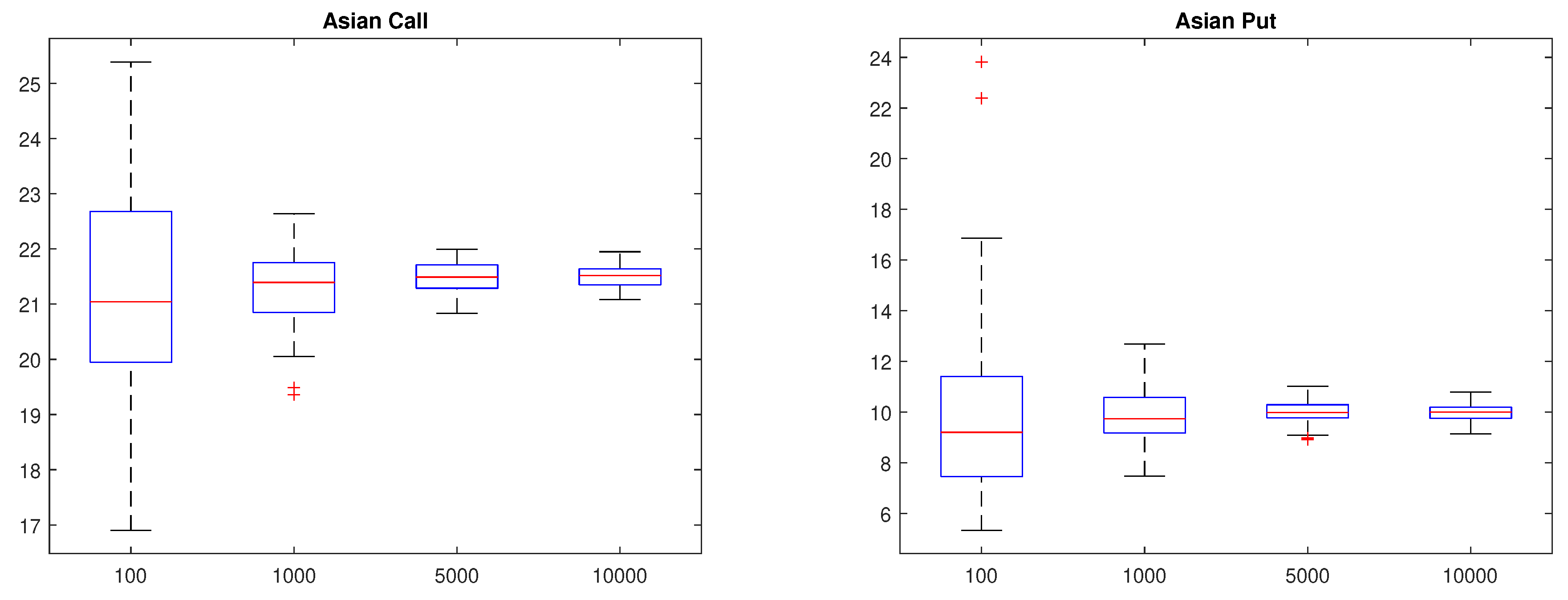
For the Asian option, we consider the arithmetic average call and put prices for strike price K = 2500 and a time to maturity of T = 25 d a y s . Table 9 shows the MCS prices for Asian call & put prices and their standard errors for simulations with 100, 1000, 5000, and 10,000 sample paths. The standard error of the MCS prices decreased as the number of sample paths increased. We repeated this process 100 times, and present boxplots for those 100 prices in Figure 8. We observe that the MCS prices converge, and dispersions are reduced as the number of sample paths increase.
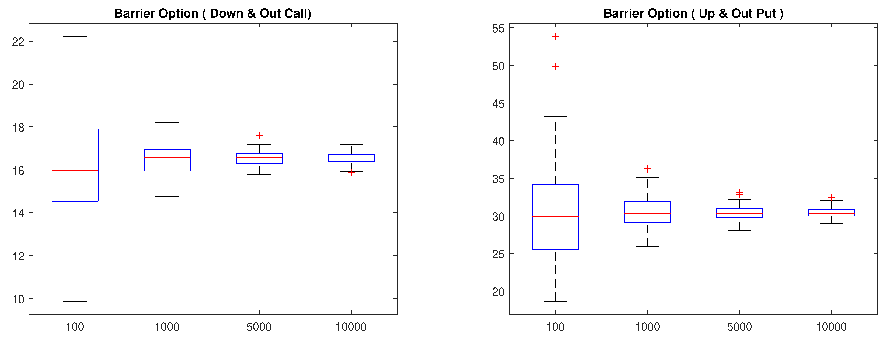
Similarly, we found the MCS price for Barrier options. We considered the down-and-out call and the up-and-out put Barrier options having a strike price of K = 2500 and time to maturity of T = 25 d a y s . Barriers of the down-and-out call and the up-and-out put are 2400, and 2750, respectively. Table 10 shows the MCS prices and their standard errors for simulations with 100, 1000, 5000, and 10,000 sample paths. The standard error of the MCS prices decreased as the number of sample paths increased. We repeated this process 100 times, and present boxplots for those 100 prices in Figure 9. We also observe that the MCS prices converged, and dispersions are reduced as the sample paths increase.

5. Conclusions

In this paper, we developed the CGMYSV sample path generation algorithm using the discrete-time approximation method with series representation. Performance of the discrete-time approximation of the CGMYSV process was tested by comparing the simulated distribution to the pdf calculated by the inverse Fourier transform method. We applied the sample path generation algorithm to European and American option pricing with MCS and LSM. We compared the MCS method to the FFT method in European option pricing with the SPX option market data. We calibrated the parameters of the CGMYSV model to the American style OEX option using LSM. We measured the performance of the calibration using four error estimators and the boot-strapping method. We conclude that the sample path generation method of the CGMYSV model performs well, and can successfully be applied to American option pricing with LSM. Finally, we also presented Asian and Barrier option pricing examples with the MCS method using the sample path generation algorithm.

Funding

This research received no external funding.

Acknowledgments

The author is grateful to Svetlozar T. Rachev and W. Brent Lindquist for their valuable discussion on this problem, and encouragement. The author gratefully acknowledges the support of GlimmAnalytics LLC and Juro Instruments Co., Ltd.

Conflicts of Interest

The authors declare no conflict of interest.

References

  1. Bianchi, Michele Leonardo, Svetlozar T. Rachev, Young Shin Kim, and Frank J. Fabozzi. 2010. Tempered infinitely divisible distributions and processes. Theory of Probability and Its Applications (TVP), Society for Industrial and Applied Mathematics (SIAM) 55: 58–86. [Google Scholar] [CrossRef] [Green Version]
  2. Black, Fischer, and Myron Scholes. 1973. The pricing of options and corporate liabilities. The Journal of Political Economy 81: 637–54. [Google Scholar] [CrossRef] [Green Version]
  3. Boyarchenko, Svetlana I., and Sergei Z. Levendorskiĭ. 2000. Option pricing for truncated Lévy processes. International Journal of Theoretical and Applied Finance 3: 549–52. [Google Scholar] [CrossRef]
  4. Carr, Peter, Hélyette Geman, Dilip B. Madan, and Marc Yor. 2002. The fine structure of asset returns: An empirical investigation. Journal of Business 75: 305–32. [Google Scholar] [CrossRef] [Green Version]
  5. Carr, Peter, Hélyette Geman, Dilip B. Madan, and Marc Yor. 2003. Stochastic volatility for Lévy processes. Mathematical Finance 13: 345–82. [Google Scholar] [CrossRef] [Green Version]
  6. Carr, Peter, and Dilip Madan. 1999. Option valuation using the fast fourier transform. Journal of Computational Finance 2: 61–73. [Google Scholar] [CrossRef] [Green Version]
  7. Cox, John C., Jonathan E. Ingersoll Jr., and Stephen A. Ross. 1985. A theory of the term structure of interest rates. Econometrica 53: 385–407. [Google Scholar] [CrossRef]
  8. Heston, Steven L. 1993. A closed-form solution for options with stochastic volatility with applications to bond and currency options. Review of Financial Studies 6: 327–43. [Google Scholar] [CrossRef] [Green Version]
  9. Hurst, Simon R., Eckhard Platen, and Svetlozar Todorov Rachev. 1999. Option pricing for a logstable asset price model. Mathematical and Computer Modeling 29: 105–19. [Google Scholar] [CrossRef]
  10. Kim, Young Shin, Svetlozar T. Rachev, Michele Leonardo Bianchi, Ivan Mitov, and Frank J. Fabozzi. 2011. Time series analysis for financial market meltdowns. Journal of Banking and Finance 35: 1879–91. [Google Scholar]
  11. Kim, Young Shin, Svetlozar T. Rachev, Michele Leonardo Bianchi, and Frank J. Fabozzi. 2010. Tempered stable and tempered infinitely divisible GARCH models. Journal of Banking and Finance 34: 2096–109. [Google Scholar] [CrossRef] [Green Version]
  12. Koponen, Ismo. 1995. Analytic approach to the problem of convergence of truncated Lévy flights towards the gaussian stochastic process. Physical Review E 52: 1197–99. [Google Scholar] [CrossRef] [PubMed]
  13. Lamberton, D., and B. Lapeyre. 1996. Introduction to Stochastic Calculus Applied Finaice. London: Chapman & Hall/CRC. [Google Scholar]
  14. Longstaff, Francis A., and Eduardo S. Schwartz. 2001. Valuing American options by simulation: A simple least-squares approach. Review of Financial Studies 14: 113–48. [Google Scholar] [CrossRef] [Green Version]
  15. Rachev, Svetlozar T., Young Shin Kim, Michele Leonardo Bianchi, and Frank J. Fabozzi. 2011. Financial Models with Lévy Processes and Volatility Clustering. New York: John Wiley & Sons. [Google Scholar]
  16. Mittnik, Stefan, Svetlozar T. Rachev, and Marc S. Paolella. 2000. Stable Paretian Models in Finance. New York: John Wiley & Sons. [Google Scholar]
  17. Rosiński, Jan. 2007. Tempering stable processes. Stochastic Processes and Their Applications 117: 677–707. [Google Scholar] [CrossRef] [Green Version]
  18. Schoutens, Wim. 2003. Lévy Processes in Finance: Pricing Financial Derivatives. Chichester: John Wiley and Sons. [Google Scholar]
1.
The class of tempered stable processes has been introduced under different names including: “truncated Lévy flight” (Koponen 1995), “KoBoL” process (Boyarchenko and Levendorskiĭ 2000), “CGMY” process (Carr et al. 2002), and classical tempered stable process (Rachev et al. 2011). Rosiński (2007) and Bianchi et al. (2010) have generalized the notion of tempered stable processes.
2.
In Carr et al. (2003), { Z t } t 0 is assumed to a CGMY process. We assume a standard CGMY process in this paper to simplify the model. The stochastic volatility Lévy process model is not a Lévy process in general.
3.
The measures are computed as follows: A A E = j = 1 N | P ^ j P j | N , A P E = j = 1 N | P ^ j P j | / N j = 1 N P ^ j / N , A R P E = 1 N j = 1 N | P ^ j P j | P ^ j , and R M S E = 1 N j = 1 N ( P ^ j P j ) 2 N , where N is the number of observations, and P ^ j and P j denote the model price and the observed market call/put prices, respectively.
Figure 1. CGMYSV sample paths (left) and CIR sample paths (right).
Jrfm 14 00077 g001
Figure 2. CGMYSV pdfs based on the simulated sample path (gray bar-plots) vs pdf using FFT method (solid curves). Distributions of X t are for t = 10 Δ t (top-left), t = 25 Δ t (top-right), t = 50 Δ t (bottom-left), and t = 100 Δ t (bottom-right), where Δ t = 1 / 252 is one day of year fraction.
Jrfm 14 00077 g002
Figure 3. Observed SPX option price and model prices calibrated to the market prices for Call (top) and put (bottom) on September 11, 2017. ‘∘’ stands for the market price and ‘+’ stands for the FFT price.
Jrfm 14 00077 g003aJrfm 14 00077 g003b
Figure 4. Confidence Intervals for the MCS option prices. Dots are observed market prices, dot-coves are MCS prices, and ‘I’ shape bars are 95% confidence intervals of MCS prices. The first (top) plate is for call option pricing and the second (bottom) plate is for put option pricing.
Jrfm 14 00077 g004
Figure 5. Bootstrapping for call (left) and put (right).
Jrfm 14 00077 g005
Figure 6. Bootstrapping for OEX put option with time to maturity of T = 31 d a y s and strike price K = 910 .
Jrfm 14 00077 g006
Figure 7. OEX put prices on April 6, 2016 and LSM prices with their confidence intervals. Circles (‘∘’) are observed OEX put prices, ‘×’ points are LMS prices, and ‘I’ shape bars are 95% confidence intervals of LMS prices.
Jrfm 14 00077 g007
Figure 8. Bootstrapping for Asian call (left) & put (right).
Jrfm 14 00077 g008
Figure 9. Bootstrapping for Barrier options: the down-and-out call (left) and the up-and-out put (right).
Jrfm 14 00077 g009
Table 1. KS test for distributions of simulated sample paths.
KS Statisticp-Value
10 days0.00700.7029
25 days0.01220.1026
50 days0.00690.7296
100 days0.01100.1748
Table 2. Calibrated Parameters for the SPX option on 11 September 2017.
ParameterCallPut
α 0.5184 0.0089
λ + 25.4592 2.0852
λ 4.6040 6.2380
κ 1.0029 1.4333
η 0.0711 0.1961
ζ 0.3443 1.1931
ρ 2.0283 0.1695
v 0 0.006381 0.0619
Table 3. Error estimators for the parameter calibration to the call and put option market price on 11 September 2017.
Call Put
ErrorFFTMCS FFTMCS
AAE 0.4442 0.6220 0.4047 0.5512
APE 0.0053 0.0074 0.0226 0.0308
ARPE 0.0711 0.0813 0.2094 0.1672
RMSE 0.6016 0.8019 0.7006 0.8608
Table 4. MCS prices and standard errors for SPX call and put with the strike price K = 2500 and time to maturity T = 28 d a y s using calibrated parameters on 11 September 2017.
Call Put
Number of SimulationPriceStandard Error PriceStandard Error
10015.96512.1001 34.33717.9356
100017.87900.7511 32.56012.2353
500019.65360.3634 32.77911.0458
10,00019.68400.2551 32.69140.7617
FFT Price19.6590 32.9541
Market Price19.05 31.50
Table 5. Parameter Calibration Results for the OEX Option market.
DateModel α C λ + λ κ η ζ v 0 ρ
Apr. 6, 2016CGMY 0.5459 0.3495 6.3595 7.7563
CGMYSV 1.1356 35.2115 7.7883 1.9322 0.3550 1.2211 0.0100 1.2237
Mar. 9, 2016CGMY 1.6885 0.0246 21.2919 2.8805
CGMYSV 0.0353 20.3911 9.9256 2.1262 0.4570 1.2665 0.0236 1.3434
Feb. 10, 2016CGMY 0.9287 3.5284 72.5855 46.4594
CGMYSV 0.0257 1.3491 0.7503 2.4301 0.4185 1.8126 0.2711 0.3567
Jan. 6, 20166CGMY 1.2290 0.4104 64.6344 21.3096
CGMYSV 1.3081 33.2233 32.5605 2.0656 0.4237 1.8947 0.0810 0.1172
Dec. 9, 2015CGMY 1.3241 0.2984 57.6574 30.2749
CGMYSV 0.6308 40.5190 24.3874 5.0247 0.3299 3.5989 0.0593 0.2334
Nov. 10, 2015CGMY 1.5907 0.0184 26.4398 2.7714
CGMYSV 0.0266 1.6365 0.7506 1.0354 0.5658 0.3936 0.1111 1.2914
Oct. 7, 2015CGMY 0.9792 0.2955 53.8624 8.4758
CGMYSV 0.8763 65.0630 67.4571 1.8555 0.2794 2.1050 0.0422 0.0080
Sep. 9, 2015CGMY 1.2572 0.5862 54.0807 15.3905
CGMYSV 0.5836 30.2731 17.2115 5.1193 0.3569 4.8231 0.1189 0.1158
Aug. 12, 2015CGMY 0.7574 0.5926 61.7876 14.2761
CGMYSV 0.4848 42.9235 31.7027 2.1644 0.1964 2.1032 0.0283 0.1639
Jul. 8, 2015CGMY 1.1742 0.2429 78.6224 11.4198
CGMYSV 0.9127 46.3671 46.3013 2.2125 0.2173 2.0394 0.0547 0.0637
Jun. 10, 2015CGMY 1.3849 0.0407 64.9276 7.8355
CGMYSV 0.0391 1.0381 0.7820 1.1451 0.6167 0.6062 0.0518 1.2736
May. 6, 2015CGMY 1.2247 0.1125 87.0744 8.6069
CGMYSV 0.8628 53.8182 54.3726 2.0949 0.2023 2.0731 0.0352 0.0647
Table 6. Error Estimates for the calibration of the OEX option.
DateModelAAEAPEARPERMSE
Apr. 6, 2016CGMY0.66230.17260.45870.8833
CGMYSV0.18810.04900.12420.2497
Mar. 9, 2016CGMY0.67800.11060.28710.8323
CGMYSV0.68330.11150.24920.8086
Feb. 10, 2016CGMY0.77550.05130.12821.1076
CGMYSV0.92670.06130.20751.2042
Jan. 6, 2016CGMY0.69450.06440.16170.9379
CGMYSV0.41400.03840.07840.6574
Dec. 9, 2015CGMY0.79860.09310.18551.1230
CGMYSV0.59030.06880.09570.7885
Nov. 10, 2015CGMY0.31370.05760.21690.4159
CGMYSV0.23370.04290.25600.3815
Oct. 7, 2015CGMY0.52680.10180.37410.6891
CGMYSV0.21860.04230.15200.3221
Sep. 9, 2015CGMY0.89480.08800.16811.2499
CGMYSV0.58740.05770.10020.9153
Aug. 12, 2015CGMY0.64640.09410.18940.9097
CGMYSV0.41370.06020.14010.5652
Jul. 8, 2015CGMY0.76360.08000.14561.0079
CGMYSV0.25180.02640.10230.3238
Jun. 10, 2015CGMY0.25350.06710.25760.3483
CGMYSV0.31800.08410.36760.4120
May. 6, 2015CGMY0.73610.07650.14790.9776
CGMYSV0.38800.04030.10970.5137
Table 7. MCS prices and standard errors for the OEX put with time to maturity of T = 31 d a y s and strike price K = 910 using parameters calibrated on 6 April 2016.
Put
Number of SimulationPriceStandard Error
10015.45652.7280
100015.03731.0173
500013.96160.3990
10,00013.87680.2856
Market Price13.950
Table 8. Numerical Summary of the bootstrapping. We repeat the MCS pricing 100 times for various number of simulation, and calculate basic statistics for the 100 MCS put prices.
Number of
SimulationMeanStdQ1Median (Q2)Q3IQRRange
10016.61193.239914.396616.558918.68504.288521.9747
100014.41900.756813.939414.434314.86090.92153.9857
500014.00730.325813.829514.025214.18760.35811.8799
10,00013.85990.252413.676613.864014.04100.36441.1730
Market Price13.950
Std: Standard Deviation, Q1: the 1st quartile, Q2: the 2nd quartile, Q3: the 3rd quartile, IQR: inter quartile range.
Table 9. MCS prices and standard errors for Asian call & put.
Call Put
Number of SimulationPriceStandard Error PriceStandard Error
10022.08341.7485 11.74003.4463
100021.00780.5866 9.70091.0759
500021.46640.2785 10.56340.5443
10,00021.65130.1937 9.99640.3679
Table 10. MCS prices and standard errors for the down-and-out call and the up-and-out put.
Down & Out Call Up & Out Put
Number of SimulationPriceStandard Error PriceStandard Error
10012.90191.4535 36.25433.6254
100015.37380.5165 30.06870.9509
500016.60970.2460 31.80300.4498
10,00016.55180.1749 30.25900.3026
Publisher’s Note: MDPI stays neutral with regard to jurisdictional claims in published maps and institutional affiliations.

