Article

An Artificial Intelligence Approach to the Valuation of American-Style Derivatives: A Use of Particle Swarm Optimization

1
Gabelli School of Business, Fordham University, 45 Columbus Avenue, New York, NY 10019, USA
2
Bank SinoPac, Financial Markets, 5F, #306, Bade Road, Section 2, Taipei 104, Taiwan
*
Author to whom correspondence should be addressed.
We thank Joe Pimbley for his encouragement and valuable comments that make this paper substantially better.
J. Risk Financial Manag. 2021, 14(2), 57; https://doi.org/10.3390/jrfm14020057
Submission received: 16 January 2021 / Accepted: 25 January 2021 / Published: 2 February 2021
(This article belongs to the Special Issue Mathematical and Empirical Finance)

Abstract

:
In this paper, we evaluate American-style, path-dependent derivatives with an artificial intelligence technique. Specifically, we use swarm intelligence to find the optimal exercise boundary for an American-style derivative. Swarm intelligence is particularly efficient (regarding computation and accuracy) in solving high-dimensional optimization problems and hence, is perfectly suitable for valuing complex American-style derivatives (e.g., multiple-asset, path-dependent) which require a high-dimensional optimal exercise boundary.
JEL Codes:
G12; G13; G4

1. Introduction

Evaluating American-style derivatives is a challenging task. In a univariate setting (e.g., option on one stock), lattice models—either the binomial model (e.g., Cox et al. 1979) or finite difference methods (e.g., see Hull 2015)—are an efficient method.1 However, once the derivative contract is written on multiple assets (e.g., exchange options), lattice models become infeasible (with regard to both computation time and memory space). Furthermore, path-dependent derivatives cannot be evaluated with lattice models.
As a result, modifying the Monte Carlo method to evaluate American-style derivatives is a popular alternative. There are two approaches to achieve this goal. The first approach is proposed by Longstaff and Schwartz (2001) who approximate the continuation value of the option by a regression function (its functional form can be arbitrary). They recognize that the early exercise decision is merely a comparison of the exercise value and its continuation value of the option. If the continuation value can be reasonably and accurately estimated, then the early exercise problem can be easily solved and hence, one can readily compute the value of an American-style derivative. The drawback of this approach is apparent—it is hard to know in advance which functional form of the regression will provide an accurate estimate for the continuation value.
The other approach is to recognize that derivatives pricing, in general, is a free-boundary PDE (partial differential equation) problem. If we can accurately estimate the exercise boundary, then it is just an easy integration over the boundary (as a first passage time problem). In other words, if we can accurately estimate the boundary, then the value of an American-style derivative can be calculated, as it would be a barrier option2.
This approach is more computationally efficient than the Longstaff–Schwartz model; yet, it suffers the same drawback of the Longstaff–Schwartz model—the accuracy of the American-style derivative value relies upon an accurate exercise boundary. Moreover, the literature of this approach lacks evidence on derivatives on multiple assets.
In this paper, we introduce an artificial intelligence method, i.e., swarm intelligence, to locate the optimal exercise boundary. In particular, we use an optimization algorithm within the realm of swarm intelligence named PSO (particle swarm optimization) to locate the optimal exercise boundary. The intelligence by the swarm can efficiently decide piecewise values of the boundary, one for each time step, without an approximated functional form as in the literature. As in any artificial intelligence model, PSO is efficient in high-dimensional optimization problems. In the case of a truly free boundary (i.e., piecewise), we find that PSO can ideally provide the best solution to complex (e.g., American-style, multi-asset, path-dependent) derivatives problems.

2. Monte Carlo in American-Style Derivative Pricing

In this section, we briefly describe the two Monte Carlo methods in American-style derivative pricing. It is generally understood that Monte Carlo simulations are only suitable for pricing European-style derivatives. This is because American-style derivatives require a backward induction. In other words, the optimal exercise decision at any given time depends on all future optimal exercise decisions. The first method proposed by Longstaff and Schwartz (2001) recreates such a recursive structure in Monte Carlo and the second method adopts a free-boundary property in PDE (partial differential equation) solutions.

2.1. The Longstaff–Schwartz Model

The Longstaff–Schwartz model (2001) is the most popular model in the financial industry. It is an efficient Monte Carlo model for American-style derivatives. Longstaff and Schwartz propose a regression method to estimate the “continuation value” at each time step.3 The option value ξ t at any time t is the larger of the exercise value E t and the continuation value C t as follows:
ξ t = max { E t , C t }
where
C t = E t Q [ ξ t + 1 ]
is the continuation value of the option at time t (which is the risk-neutral expected value, E t Q [ ] , of the next period’s option price); and E t is the exercise value at time t . In the case of a put option (which is what we use throughout the paper), E t = K S t .
Longstaff and Schwartz cleverly recognize that the conditional expectation of future maximum payoff is a function of today’s stock price:
E t Q [ ξ t + 1 ] = f ( S t )
where f ( ) is an arbitrary function. They propose the simplest (and it works amazingly well) quadratic equation:
E t Q [ ξ t + 1 ] = f ( S t ) = a 0 + a 1 S t + a 2 S t 2
which can turn into a regression model as follows:
ξ t + 1 = a 0 + a 1 S t + a 2 S t 2 + e t + 1
with the boundary condition ξ T = max { K S T , 0 } .
As mentioned earlier, the major criticism of the model is the choice of the functional form of the regression. It is ad hoc and it is not possible to know which form is most suitable for which payoff.4

2.2. Explicit Boundary Method

In an alternative (relatively unsuccessful) attempt, researchers have tried to solve American-style derivatives by using an explicit exercise boundary5. The approach is built upon the advantageous property that option prices of any kind are solutions to a class of differential equations which can be solved as a “free boundary problem”. In other words, as long as the exercise boundary of an option is known, its price is no more than a simple integration along the exercise boundary.
Unfortunately, not only is the exercise boundary of an American-style derivative unknown, but it is recursive (i.e., the boundary value at the current time depends on the boundary value at the immediately later time—resulting a recursively dependent structure of boundary values). In other words, the boundary function can only be achieved via a lattice model (e.g., binomial model). In doing so, the option is guaranteed to be exercised optimally and the valuation can hence be at the maximum.
As Carr (1998), among others, points out, if we solve an American-style derivative premium as a free-boundary problem, then we can use an explicit boundary function and the American-style derivative premium is simply an integration of payoff function (e.g., put) over the boundary.
ξ ( t ) = E t Q [ e r τ max { [ E ( τ ) , 0 } ]
where E ( τ ) is the exercise value at the stopping time τ . If it is a put option without dividends, which is the case in this paper, then E ( τ ) = K S ( τ ) . On the boundary, S ( τ ) = B ( τ ) and hence, E ( τ ) = K B ( τ ) where B ( τ ) is the boundary function given exogenously. The way the boundary function works is that it serves as a stopping time. Once the stock price at time t hits the boundary B ( t ) , the process stops and the option will be exercised and paid and hence, the American-style derivative can be evaluated as a barrier option.
The easiest way to perform the integration is through Monte Carlo simulations. As the derivative price, ξ ( t ) is given as an expected value:
ξ ( t ) = 1 N j = 1 N e r τ j max { K B ( τ j ) , 0 }
We note that the recursively determined boundary function (via a lattice model) maximizes the option value; any other exogenously specified boundary function will only be “sub-optimal”, that is, generating a lower value than the lattice model. This sub-optimal argument is convenient in that now we can simply try a large number of boundary functions and use the one that generates the highest option value as a good approximation.
Researchers then have tried various approximations on the exercise boundary. These approximations are explicit functions and hence, can be easily integrated (thus, the American-style derivative value can be solved). According to a recent survey by Nunes (2009), the literature has the following functional forms:
  • Constant: B ( t ) = a 0 ;
  • Linear: B ( t ) = a 0 + a 1 t ;
  • Exponential: B ( t ) = a o e a 1 t ;
  • Exponential-constant: a 0 + e a 1 t ;
  • Polynomial: B ( t ) = i = 1 n a i t i 1 ;
  • Carr et al. (2008): B ( t ) = min ( K , r q K ) e a T t + E [ 1 e a T t ] .
Note that the boundary is not a function of the stock price (i.e., free boundary problem). Since these boundary functions are explicit, they can be easily integrated.
Certainly, the accuracy of the American value depends on the accuracy of the approximated boundary function. The problem of this approach is that there is no consensus of which functional form of the boundary can consistently be the best. Often, it varies with the parameters of the option (i.e., moneyness, interest rate, time to maturity, and volatility). As a result, no conclusion can be drawn on a particular functional form.
So far, the literature has not reached any consensus and the boundary seems to be payoff-specific. In other words, different payoffs require different boundaries for accurate American-style derivative values. As a result, it is quite natural to allow the boundary function to be absolutely free (i.e., one value per time step). Yet, this requires an optimization in high dimensions. As the number of time steps increases, the cost of computation becomes exponentially and prohibitively high.
In this paper, we propose an artificial intelligence (AI) method which is based upon the theory of swarm (swarm intelligence, SI). In the SI model, a school of fish (or a group of ants and bees or a flock of birds) will move (swim) around to look for the maximum value of the option.

3. Swarm Intelligence

In this section, we briefly “open the black-box” of swarm intelligence, which is a branch of recently popular artificial intelligence.

3.1. What is AI?

Artificial intelligence (AI), machine learning (ML), and big data (BD) have recently been adopted into FinTech and have been the fastest growing area in finance, both in private industry and academia. While these three areas are frequently used in combination in developing valuable applications, these three areas are fundamentally different and deserve separate research.
Strictly speaking, AI is a combination of computation (artificial) and biology (intelligence), which is quite different in nature from ML which is based upon statistical methodologies. In the past, statistics have predominantly been presented in a parametric fashion, mainly due to insufficient computational power and lack of data. This has been changed recently and non-parametric statistics with powerful computation capabilities have fueled the growth of machine learning. As non-parametric statistics require a large amount of data, ML and BD (such as NLP, or natural language processing) have been combined in revolutionizing the financial world. Together, they facilitate the progress of AI.
AI has four major branches:
  • Swarm intelligence (birds, ants, bees, fish);
  • Genetic algorithm (genes);
  • Neural networks (neurons);
  • Reinforcement learning (mice in a maze).
These AI theories are behavioral models in that they “artificialize” natural intelligence (specified in parentheses above) which reflects biological behaviors. As a result, they are different from ML methodologies. The connection (and hence, confusion) of these two is due to the fact that these AI models can be efficiently used to find optimal solutions (e.g., PSO) which then are similar to ML models. Indeed, from the perspective of computation, one can hardly differentiate one tool from the other and in many instances, these two distinctly different theories are used in combination.
As we shall demonstrate in this section, swarm intelligence is a behavioral model and PSO is an optimization tool.

3.2. Swarm Intelligence

Wikipedia describes swarm intelligence as “the collective behavior of decentralized, self-organized systems.”6 The basic idea of swarm intelligence is derived from those animals (such as birds, ants, bees, and fish) that rely on a group effort to achieve their basic survival needs—seek food and avoid prey. The intelligence behind this collective behavior is how they communicate among one another. Reynolds (1987)7 was the first to “artificialize” such natural intelligence and create a computer algorithm named Boids (bird-oid object). Reynold’s algorithm is amazingly simple. For any given bird, Reynold devises a set of linear equations (vectors), combining which determines how the bird should fly to its next destination.
The factors that determine how various vectors are combined are: separation, alignment, and cohesion. As their names suggest, “separation” is to avoid collision with other birds, “alignment” decides how a particular bird should fly in a direction by referencing to its fellow birds, and “cohesion” decides how fast (speed) a particular bird should fly to its next target position.
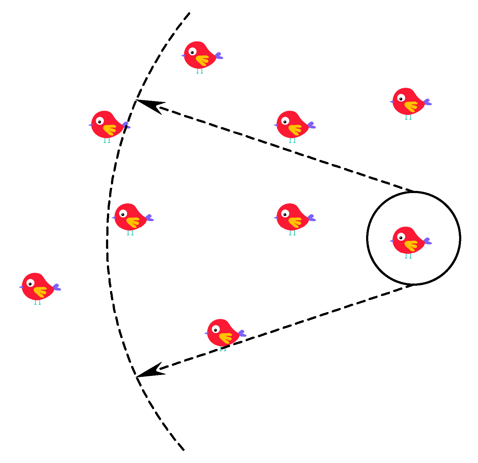
There are countless versions of Boids.8 One can add obstacles. One can add an objective destination (swim to target). One can perform Boids in a maze. The basic Boids, as described in Figure 1, can be described by the following algorithm.
Formally, let there be m birds flying in an n -dimensional space. Also let:
  • f t ( i ) be the i th bird at time t ;
  • v t ( i ) be a vector in the n space representing the velocity of the i th bird;
  • p t ( i ) be a vector in n space representing the position (coordinates) of the i th bird.
Finally, let F = { f t ( i ) | i = 1 , , m } be the collection of all birds. Define a mapping function X i = ( f t 1 ( i ) ) , which returns all of f t 1 ( j i ) F f t 1 ( i ) , where a radius d and an angle a are predetermined ( | | x , y | | = x 2 + y 2 , and { x , y } is the angle between two vectors), such that
| | v t 1 ( i ) , v t 1 ( j i ) | | < d | | p t 1 ( i ) , p t 1 ( j i ) | | < d   and   { v   and   t 1 ( j i ) , v t 1 ( i ) } = a ° { p t 1 ( j i ) , p t 1 ( i ) } = a °
are satisfied. In words, what (8) describes is that for any given bird i , where it is heading depends on a reference group of birds “nearby”, described by a set of birds X i = ( f t 1 ( i ) ) . These reference birds must be “nearby” in the following sense—they must be within a distance (specified by the radius d ) and within an angle (specified by a ° ), as depicted graphically as9:
Jrfm 14 00057 i001 where the circled bird is referencing three nearby birds by the angle and the radius. The alignment and cohesion (we ignore the separation parameter for the moment) parameters are calculated as follows10:
v A , t ( i ) = avg ( v t 1 ( j i ) | f t 1 ( j ) X ) v t 1 ( i ) v C , t ( i ) = avg ( p t 1 ( j i ) | f t 1 ( j ) X ) p t 1 ( i )
Then, an average velocity is calculated as follows:
v ¯ t ( i ) = w A v A , t ( i ) + w C v C , t ( i )
where w A + w C = 1 and each is positive. Finally, the velocity and the position of each bird are updated as follows:
v t ( i ) = v t 1 ( i ) + v ¯ t ( i ) p t ( i ) = p t 1 ( i ) + v ¯ t ( i )
As emphasized earlier, a swarm is a behavioral model which describes how birds (ants, bees, fish) move and an artificial swarm is a mathematical (linear algebraical) algorithm that imitates this natural behavior by animals. One can use an artificial swarm to solve a number of complex problems.11
As we can see, Reynold’s boid model can be easily programmed and implemented. For the sake of easy exposition, we shall refer to birds, ants, bees, or fish as particles for the rest of the paper.
Particle Swarm Optimization (PSO) can be viewed as a simplified AI swarm. Its objective is to find the global optimum. While details can be seen in the next section, the idea of PSO is to replace nearby birds/particles with the global optimum found by all birds/particles.

3.3. Particle Swarm Optimization

In theory, swarm intelligence is effective for optimization problems in a high-dimensional space. PSO is such an application. The original version of PSO was first proposed by Eberhart and Kennedy (1995) who modify the behavioral model of swarm into an objective-seeking algorithm. Similar to Reynold’s, their model “artificializes” the group behavior of a flock of birds seeking food. Via bird-to-bird chirping (peer-to-peer communication), all birds fly to the loudest sound of chirping. Subsequently, Eberhart and Shi (1998) improve the model by adding an inertia term (symbolized as w later as we introduce the model) and this has become the standard PSO algorithm used today. Setting a proper value of the inertia term is to seek the balance between exploitation and exploration. A larger value of the inertia term gives more weight to exploration (as the bird is more likely to fly on its own) and a smaller value of the inertia term gives more weight to exploitation (as the bird tends more to fly toward other birds).12
One can compare PSO to a grid search. A grid search can find the global optimum and yet, it takes an exploding amount of time to reach such a solution, especially in a high-dimensional space. PSO can be regarded as a “smart grid search” where each particle performs a “stupid search” and yet, by communicating with other particles and by having a large number of such particles, we can reach the global optimum quickly.
Imagine we would like to measure the deepest place of a lake whose bottom has an uneven surface. A two-dimension grid search can easily find the global minimum. An alternative would be PSO. Imagine we have a number of “fish” (particles) who swim in the lake. At each time step, all fish will measure the depth of the lake underneath them. Each fish is communicating with all the other fish to decide whose depth is the deepest (minimum). All fish now remember the minimum and then they swim for another time step. At each time step, they update the global minimum so far. If we let these fish swim randomly for enough time, we will reach the global minimum.
In the case of the lake, we may find grid search to be more accurate and time-effective. However, in an n-dimensional lake, grid searches become ineffective; the same number of fish may just perform the same job in the same amount of time as in the two-dimensional lake.
Currently there have been a limited number of applications of PSO in finance, mostly in portfolio selection. In this paper, we use it for the first time in the literature to locate the exercise boundary of American-style derivatives (specifically, put options, options on min/max, and Asian options).13
The PSO algorithm can be formally defined as follows. For i = 1 , , n particles, and each particle is a vector of j = 1 , , m dimensions, we have:
{ v i , j ( t + 1 ) = w ( t ) v i , j ( t ) + r 1 c 1 ( p i , j ( t ) x i ( t ) ) + r 2 c 2 ( g ( t ) x i , j ( t ) ) x i , j ( t + 1 ) = x i , j ( t ) + v i , j ( t + 1 )
where v i , j ( t ) is the velocity of the i th particle in the j th dimension at time t ; x i , j ( t ) is position of the i th particle in the j th dimension at time t ; w ( t ) is a “weight” (less than 1) which decides how the current velocity will be carried over to the next period (and usually, it is set as w ( t ) = α w ( t 1 ) and α < 1 to introduce diminishing velocity);14 and finally, r 1 , r 2 ~ u ( 0 , 1 ) follow a uniform distribution.
In the swam literature, w ( t ) v i ( t ) is called inertia; r 1 c 1 ( p i ( t ) x i ( t ) ) is called the cognitive component; r 2 c 2 ( g ( t ) x i ( t ) ) is called the social component. Coefficients c 1 and c 2 are known as acceleration coefficients.
At each position, there is a “cost function” f ( ) (sometimes called distance function), at which a “cost” (or penalty) is computed. This cost function is the objective function to be minimized (or maximized).
The global best at any given time is either the maximum or minimum value of the objective function generated by all particles at the time:
g ( t ) = min i { f ( p i ( t ) ) }
and the personal best at the time is:
p i ( t ) = min t { f ( x i ( t ) ) }
and f ( ) : n is the “fitness function”. The usual fitness function is
f ( x i ( t ) ) = x i χ _ = j = 1 J ( x i j χ j ) 2
where χ _ = < χ 1 , , χ J > is a coordinate in a J -dimensional space.
Later, we illustrate via a very simple example how the process is so easily implemented.
As we can see, the algorithm (at least, the standard one presented here) of PSO is quite different from that of a generic swarm by Reynolds (1987). Yet, they both share the same behavioral pattern of a natural swarm. In other words, (1) both PSO and the generic swarm are based upon peer-to-peer communication in order to achieve the objective and (2) the particles in both PSO and the generic swarm are identical (like birds or ants) and each particle follows its neighbor particles. The difference is just how each particle weighs its neighbors. In PSO, each particle only cares about the global best discovered by its neighbors; in the generic swarm, each neighbor’s position is important.
(i) Different Types of PSO
The literature on PSO is voluminous. Zhang et al. (2015) provide an excellent survey. They classify the existing PSO literature into the following strands:15
  • Modifications;16
  • Population topology;17
  • Hybridization;18
  • Extensions;19
  • Theoretical analysis;20
  • Parallel implementation.21
However, Zhang, Wang, and Ji only provide applications in non-financial areas.22, 23 To date, there have been a very limited number of applications in the area of finance. Within the limited literature, most noticeable is the area of portfolio selection.24
(ii) A PSO Demonstration
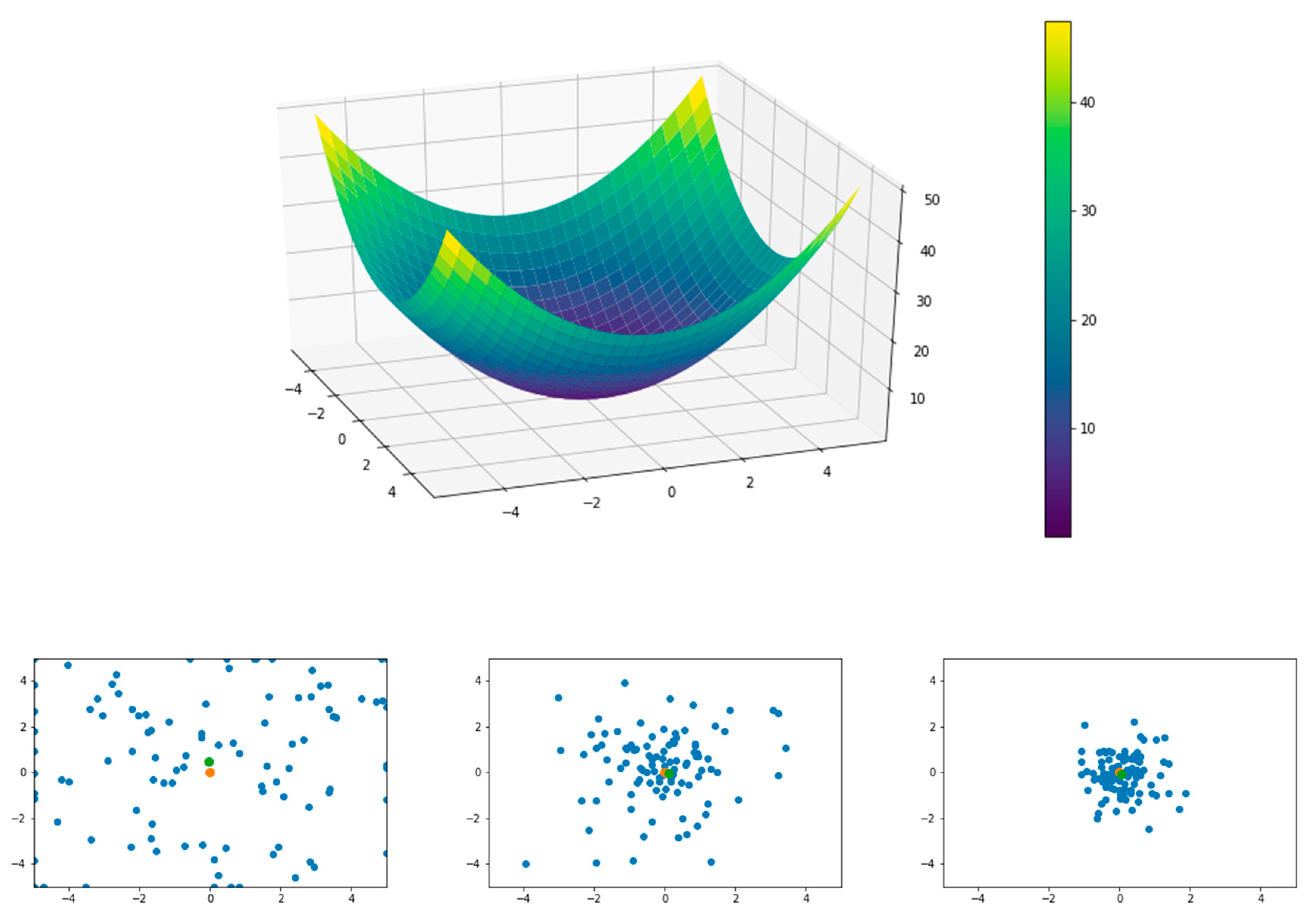
As a demonstration, we use a conic function as follows:
f ( x , y ) = x 2 + y 2
The function is a cone, as shown in the top plot in Figure 2. In Figure 2a, we can readily see how particles move toward the center of the cone, which is the global minimum.
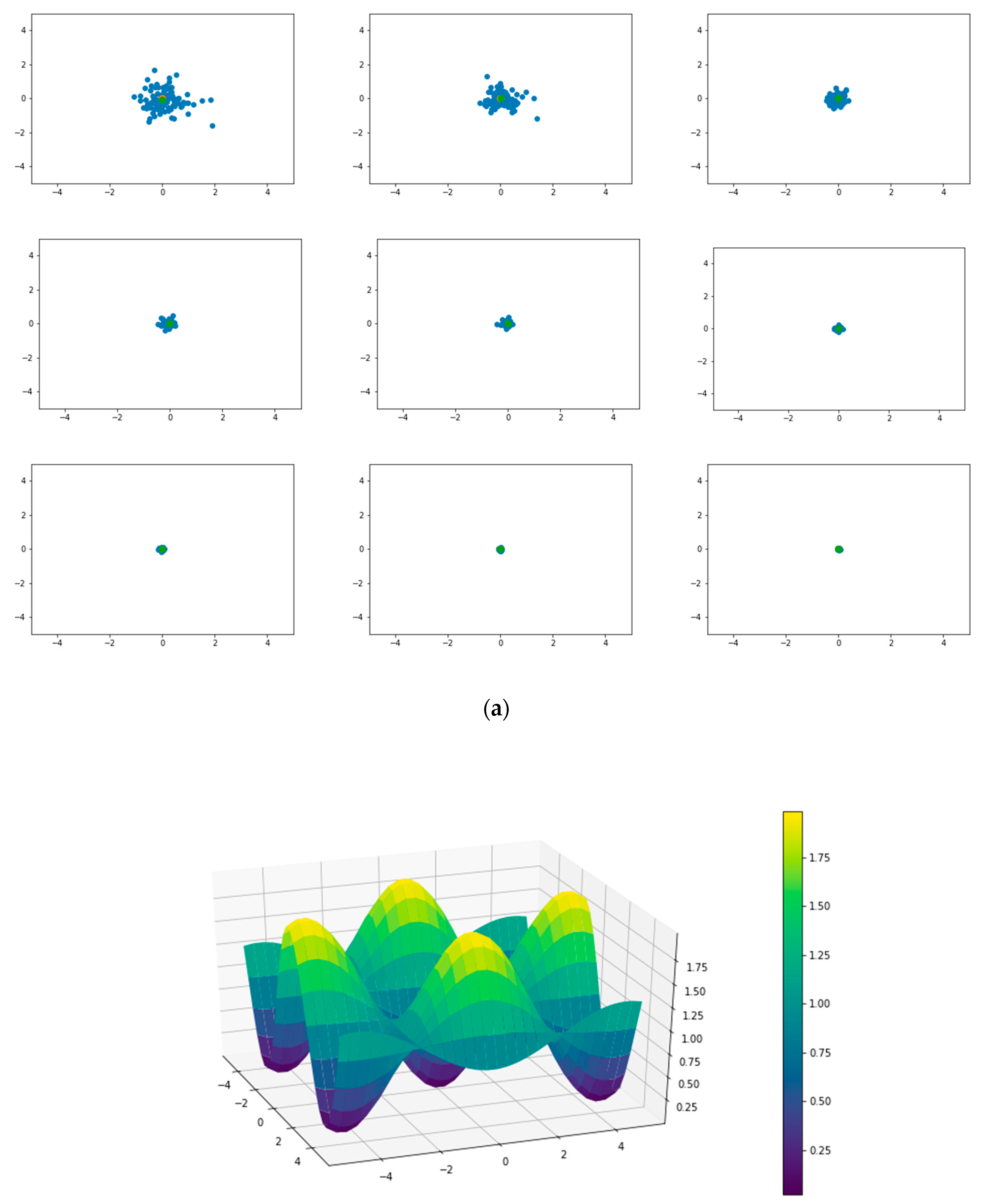
Another function, as follows, has multiple local minima.
f ( x , y ) = x 2 + y 2 4000 cos [ x ] cos [ x 2 ] + 1
Results are shown in Figure 2b.
The major advantage of PSO is that it is particularly good for problems with many local optima, as we can see in Figure 2b. However, in this situation, the convergence of the swarm is slower, and each particle needs to “work harder” to identify the global minimum, since there are many local minima.
Another advantage of PSO is its superior capability to find the global optimum when the objective function is discrete. In Huang (2019), PSO is applied on the maximization of the Sortino ratio. Different from the Sharpe ratio, the Sortino ratio only concerns the “down-side risk” and as a result, the ratio is not a continuous function of the portfolio weights.
Thirdly, PSO is insensitive to initial value. However, given the heuristic nature of PSO (or any AI-based optimization), accuracies are not as good as competing parametric methods. As a result, PSO is best used in high-dimensional problems where parametric methods fail. In this paper, we demonstrate how PSO can be used in evaluating complex derivatives. These complex derivatives usually require optimization through a high-dimensional search, which leads to failures (or highly inaccurate estimates) by the parametric methods. For the sake of easy exposition, we demonstrate simple American-style options such as put, put on min/max, and Asian options.

4. American-style Derivative Pricing

As mentioned earlier, once the exercise boundary can be correctly specified, one can perform Monte Carlo simulations to solve for American-style derivative prices. Moreover, with this capability, one can further solve path-dependent options which are impossible to be solved by lattice models. Also mentioned earlier is the difficulty, admitted in the literature, of how to identify such a truly free exercise boundary. In this section, we demonstrate how to take advantage of PSO to achieve this goal. In PSO, there is no need to specify any functional form for the exercise boundary. Particles will collectively set the exercise boundary with no constraints, which in theory gives the best American-style derivative value.
We first demonstrate a simple American put option on one and two assets where there are accurate estimates via a lattice model. Then, we demonstrate a path-dependent option (Asian option) that cannot be evaluated easily by lattice models.

4.1. Univariate

We first demonstrate how PSO is used in a simple American put option without dividends. In this simple example, we can have the lattice result (binomial model) as the benchmark. With the help of the binomial model, we can clearly see the exercise boundary of the option. The input information to the American put option is as follows:
Scheme 100.100
strike price100
volatility0.3
risk-free rate0.03
time to maturity1
time steps100
Monte Carlo paths10,000
Given that the binomial model and the PSO use the same number of time steps, we caution that the binomial model does not provide accurate enough results due to not having enough steps (only 100).25
We use PSO to evaluate various boundary specifications. Specifically, for any given boundary specification (i.e., flat, linear, exponential, piecewise flat, and restricted piecewise flat), we maximize Equation (7) over
max Θ ξ ( t )
where Θ represents the set of parameters of the boundary function and ξ ( t ) is the option value defined in Equation (7):
ξ ( t ) = 1 N j = 1 N e r τ j max { K B ( τ j ) , 0 }
For example, in the linear boundary case, Θ = { a 0 , a 1 } . Hence, Equation (18) is a two-dimensional search. Note that B ( τ j ) is the boundary value of the jth path at time τ j . Take a concrete example. Given a boundary specification (e.g., linear B ( t ) = a 0 + a 1 t ), τ 5 (the fifth path) could be time step 26, and τ 42 (the forty-second path) could be time step 74.26 The boundary values are consequently B ( τ 5 ) = a 0 + a 1 T 26 and B ( τ 42 ) = a 0 + a 1 T 74 . In other words, at the fifth path of Monte Carlo, the option is exercised early at step 26, and the exercise value is equal to K B ( τ 5 ) = K ( a 0 + 0.26 a 1 ) . Similarly, at the forty-second path of the Monte Carlo, the option is exercised early at step 74, and the exercise value is K B ( τ 42 ) = K ( a 0 + 0.74 a 1 ) .
Note that in the piecewise flat boundary case, there is no formula, and each time period has its own boundary value. In this case, Θ = { B 1 , , B 100 } and Equation (18) is a 100-dimension search. In PSO, each particle is labeled with 100 coordinates. The particles communicate with one another to update their coordinates (global best) at each iteration. Iterations stop when all particles converge to the same set of coordinates and Equation (18) is maximized.
We compare different boundary conditions. The results are given in Table 1.
The European value is 10.3656 by the Monte Carlo method, which is a little higher than the true value of 10.3278 by the Black–Scholes model. The binomial value for the European option is 10.2984, which is lower than the Black–Scholes value. Hence, we can infer that the American value, which is 10.5917 by the binomial model, should be underestimated. Thus, we can view the binomial value as a lower bound.
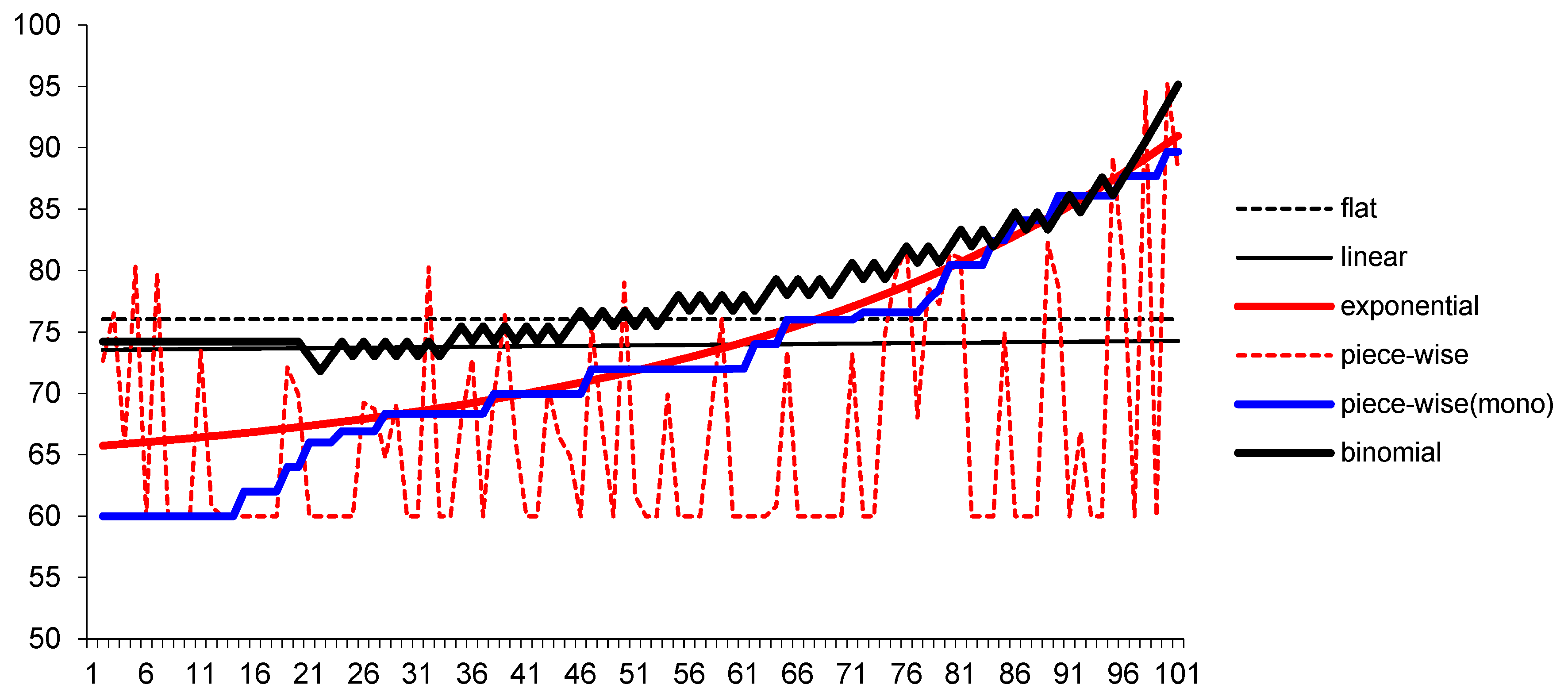
The piecewise PSO value is 10.7714, which is the highest American value, as expected as it imposes no restriction. The restricted (monotonically) piecewise PSO value is the next highest at 10.6908. Given that the true exercise boundary is very close to an exponential function (provided later in Figure 3), the exponential boundary result of 10.6647 should be very close to the true value.
The Longstaff–Schwartz value (regression, which uses Equation (5)) is 10.6217, which is lower than the above three results but higher than the linear boundary result of 10.5621 and the flat boundary result of 10.5591. These results seem reasonable.
We then compare the exercise boundaries from the various specifications and compare them to the “true exercise boundary” implied by the binomial model. The exercise boundary is plotted in Figure 3.
Figure 3 it is clear that the exercise boundaries implied by the binomial, exponential, and piecewise-monotonic cases are close to one another. The unrestricted piecewise boundary is also close if we ignore the low values but only focus on the high values. The unrestricted piecewise boundary oscillates but clearly those low values have little impact on the valuation (as we can see from the result that this boundary yields the highest American-style derivative value in Table 1). The flat and linear boundaries perform poorly (Table 1) as no surprise as they are far from the correct boundary.
Clearly, both PSO and binomial algorithms can be improved. First, the zigzag form of the binomial boundary is disturbing.27 This could be due to insufficient number of periods (which confirms the slow convergence of the binomial model). Second, there are a substantial number of low values (at 60) by the unrestricted piecewise boundary. It is clear that these values are bad values and yet it does not impact the valuation much, which indicates that the exercise boundary does not need to be granular. This is a numerical issue worthy of further investigation. Yet it is future research and beyond the scope of the current paper.

4.2. Multivariate

There are a number of multivariate lattice models. In principle, the challenge in building such a multi-dimensional lattice is the exploding memory usage and computation time. In the simplest case where all assets are uncorrelated, the number of nodes necessary for the lattice is ( ( m 1 ) t + 1 ) n , where m is the number of economic states for any given asset, n is the number of assets, and t is the number of time steps in the lattice. For example, in a trinomial lattice, using 100 time steps to evaluate a three-asset derivative requires over 8 million nodes at maturity.28
Another challenge for building a multivariate lattice is the difficulty in incorporating the number of pair-correlations of assets. In other words, it is not possible to match the number of equations (i.e., branches) and the number of unknowns (i.e., correlation pairs).29 In the simplest case where assets are independent, we need 2 n branches (where n is the number of assets) in each time step. In order to incorporate correlation, Boyle (1988) and then, modified by Kamrad and Ritchken (1991), devised a five-branch model. The corner branches have the same stock prices as before and the middle branch assumes the same stock prices as the current. By matching moments, there are six equations and five unknowns. Hence, the solution is not so straightforward. Boyle (1988) shows that the usual binomial setup with two assets X and Y ,30 that is, X u = X 0 u X = X 0 e σ X Δ t and X d = X 0 d X = X 0 e σ X Δ t and similarly, for Y . Due to the mismatch of equations and unknowns, the assumption must be altered to u X = e λ σ X Δ t and u Y = e λ σ Y Δ t , where λ is a free parameter so that this can be solve for one stock first and then, the solution to the second stock can be searched for.
The second model by Boyle et al. (1989) is a four-branch model. As we can see, if we use four branches (i.e., four equations), we will not be able to match unknowns and equations. Hence, Boyle, Evnine, and Gibbs turn to characteristic functions. They note that the above probabilities can all be nonnegative only if the time step becomes sufficiently small. Hence, this method is not very efficient.
Finally is the model by Chen et al. (2002). Their model is based upon complete markets. In a complete market, the number of nodes does not grow exponentially but factorially, which saves both computation time and memory usage. Furthermore, the complete market setting is consistent with the binomial model in a single asset case and as a result, risk-free no-arbitrage can be established. In other words, like the binomial model, the Chen–Chung–Yang model is not just a numerical algorithm as with Boyle (1988), Boyle et al. (1989), and Kamrad–Ritchken, but also an economic model.
In the complete market setting, Chen et al. (2002) discovered that the number of branches in each time step exactly matches the number of equations. Consequently, one can easily solve for the probabilities as in the binomial model. While the readers can find all the details in their original paper, in the Appendix, we excerpt a two-asset example where the two-dimensional “binomial tree” can be visualized.
We evaluate the following put option (note that the call option will never be exercised early):
V τ = max { K max { S 1 τ , S 2 , τ } , 0 }
with the parameters of the two stocks given as:
asset 1asset 2
price4040
volatility0.20.3
strike35
time to maturity7/12
risk free rate0.03
correlation0.5
Implementing the PSO algorithm, we recognize that there is a certain relationship between functions B 1 , τ and B 2 , τ . For example, it could be: B 1 , τ = a + b B 2 , τ (linear) or a 2 B 1 , τ 2 + b 2 B 2 , τ 2 = c 2 (elliptical/concave), where a , b , and c are arbitrary constants, along with B 2 , τ to be decided by PSO. In the current execution, we assume B 1 , τ and B 2 , τ to be independent.
The results are given in Table 2. In Table 2, we also implement the Longstaff–Schwartz model with the following quadratic regression (compared to Equation (5)):
ξ t + 1 = a 0 + a 11 S 1 t + a 12 S 1 t 2 + a 21 S 2 t + a 22 S 2 t 2 + a 3 S 1 t S 2 t
Similar to Table 1, we find the PSO results and the Longstaff–Schwartz result to be very close to each other. The Black–Scholes European value is 0.1948 and the binomial American value (i.e., the Chen–Chung–Yang model) is 0.2557 with a European value as 0.1884. Hence, we know that the American value by the binomial model is underestimated.
The Monte Carlo European value is 0.1974, which is close to the Black–Scholes value. The Longstaff–Schwartz value is 0.2386, which is lower than the binomial value. Among all PSO values, again, the unrestricted piecewise boundary yields the highest value of 0.2426, followed by the exponential boundary of 0.2361. The flat boundary continues to be the worst case at a value of 0.2318. It is quite surprising to see that the exponential boundary yields a higher option value than the piecewise monotonic boundary of 0.2352.

4.3. Path-Dependent

The lattice approach for the valuation of American-style derivatives does not apply to those contracts whose payoffs depend on past values (i.e., path-dependent options). On the other hand, Monte Carlo simulations are good for European path-dependent options. Yet, there has been no good approach to evaluate American path-dependent options.
Asian (Averaging) Option
We use the simple Asian option as a demonstration. An Asian option is an option whose payoff depends on a historical average (arithmetic or geometric, weighted or unweighted) of past values of the underlying asset. As a result, an Asian option cannot be evaluated using the standard lattice method, in that a lattice does not keep track of the historical values of the underlying asset. As a result, a Monte Carlo algorithm must be employed. However, the Monte Carlo method cannot evaluate American-style options. As a result, evaluating American-style Asian options remains a challenge.
To date, there has been no other alternative to the Longstaff and Schwartz (2001) model which provides an approximation value to the American-style Asian option. In this paper, a more superior alternative, using PSO, is proposed.
First, we have to turn the valuation to a free-boundary problem. As discussed earlier, PSO is suitable to evaluate any free-boundary valuation problem. An American-style Asian option has the following payoff:
V τ = max { A τ K , 0 }
where τ is the (early) exercise date and
A τ = 1 n i = 0 n 1 S τ i
is the average of the stock price (in this example, the average is arithmetic). An American-style Asian option is to compare the above exercise value against the continuation value. This nature, which is same for all American options, now is applicable to Asian options. In other words, there exists a critical value touching which triggers the early exercise. Hence, we can now use PSO to locate the exercise boundary.
Note that now the exercise boundary is located along the averaging value path A τ . In Monte Carlo simulations, this can be handled along each path with no difficulty. Valuation can be performed on A τ just as it is on S t . The results are in Table 3.
There is no closed-form solution to the European-style Asian option evaluated here, nor is there a benchmark American value by the lattice model. Without knowing a benchmark, we cannot assess the accuracy of various PSO results and the Longstaff–Schwartz result. Hence, Table 3 can only provide a comparison between the results by Longstaff–Schwartz and PSO.
First, we can see that flat, linear, and exponential boundaries can hardly be accurate in that they generate an identical value to the American-style derivative (9.0117) which is very close to the European value (9.0109). Secondly, piecewise boundaries, restricted and unrestricted, both provide substantially higher values than the other three cases—9.1912 and 9.1925, respectively. This indicates that we obtain a substantially higher value once the boundary function is flexible. Lastly, the Longstaff–Schwartz value is the highest (9.2415) and yet, it is unclear if their value overestimates or underestimates the true value. Hence, it is unable to assess the performance in this situation.

4.4. Computational Efficiency

In this section, we examine the issue of computation efficiency. In general, AI-based algorithms are not fast. As a result, computational efficiencies can be gained only in high dimensions. This is because the increase in dimensionalities and the increase in particles are both linearly proportional to computation time. This is sharply different from the traditional methods that suffer the well-known “dimensionality curse” where the increase in dimensions results in exploding computational time. As a result, there is no benefit in using an AI-based model in low dimensions.
Table 4 presents the results of (A) a simple American put option and (B) an American put option on two assets in various simulations. For 100 particles, the computation time ranges from 25.10 to 46.88 s (with different seeds). Note that there is no clear relationship between the accuracy of values and speed. The fastest seed (#3143) takes 25.10 s but produces the second highest value; while the slowest seed (#41675) takes 46.88 s but produces the third highest value.
We have the following observations. First, given the heuristic nature of PSO, we provide results with various Monte Carlo seeds. As we can see, the variation in results is non-trivial. Different Monte Carlo paths affect the results quite substantially. Fortunately, we can observe a pleasant pattern in mean (average across seeds), max (maximum across seeds), and min (minimum across seeds). In these results, more particles (higher swarm size) do take longer to compute and do converge to more accurate results (option values).
Secondly, and more interestingly, we do not find differences in computation times between Panel A, which is the option on the single asset and Panel B, which is the option on two assets. This confirms the conjecture that PSO is not significantly affected by the number of assets. This is drastically different from previous models where dimensionality matters. For example, for a swarm size of 100, the mean computation times are 37.48 s for one asset and 40.82 s for two assets.
Lastly, note that one of the advantages of PSO is that computation time is linearly related to swarm size (number of particles). Hence, to increase accuracy, we can simply increase the swarm size, and the cost only increases linearly. For example, the average speed for a swarm size of 50 is 20.71 s and for a swarm size of 500 is 229.67 which is roughly 10 times more (and similarly, a swarm size of 100 is roughly double (46.88 s) and a swarm size of 200 is four times (87.67 s)).

5. Conclusions

In this paper, we demonstrate how complex (multi-asset or path-dependent) American-style derivatives can benefit from an artificial intelligent tool—PSO (particle swarm optimization). These options are otherwise nearly impossible to evaluate accurately and efficiently. In other words, PSO is particularly suitable for evaluating these complex derivatives.
PSO is an optimization tool particularly suitable for high-dimensional problems. Compared to other optimization tools (e.g., stochastic gradient descent), PSO is intelligence-based. One can regard PSO (or any intelligence-based tools such as genetic algorithms and neutral networks) as “non-parametric”, and other optimization tools (e.g., stochastic gradient descend) as “parametric”. This analogy points out that PSO has more flexibility and can more likely find the better value.
Another extraordinary advantage of PSO is its capability in parallel computing. In other words, PSO can be GPU-ized (graphic processing unit). This indicates that the computation time of PSO can be infinitely minimized (by adding GPUs). Experiments on GPU computation are beyond the scope of this paper.
We also discover, presented in Table 4, PSO is quite sensitive to Monte Carlo paths. Particles behave quite differently in a different environment. This opens the door for another future research work.

Author Contributions

R.-R.C. and J.H. jointly developed the idea using PSO to price American options. R.Y. helped derive the exercise boundaries in complex options. W.H. contributed in experimenting various PSO varieties. All authors have read and agreed to the published version of the manuscript.

Funding

This research received no external funding.

Conflicts of Interest

The authors declare no conflict of interest.

Appendix A

Appendix A.1. American Call Option on Min/Max Will Never be Exercised Early

Jansen’s Inequality states that if f ( x ) is a convex function, then f ( E [ x ] ) E [ f ( x ) ] and vice versa. Hence, the American call option will never be exercised early. It is well-known that the simple call option’s continuation value is always greater than the exercise value:
e r Δ t E [ max { S T K , 0 } ] e r Δ t max { E [ S T ] K , 0 } = max { e r Δ t E [ S T ] e r Δ t K , 0 } > max { S T 1 K , 0 }
In addition, the exchange option will never be exercised.
e r Δ t E [ max { S 1 , T S 2 , T , 0 } ] e r Δ t max { E [ S 1 , T ] E [ S 2 , T ] , 0 } = max { e r Δ t E [ S 1 , T ] e r Δ t E [ S 2 , T ] , 0 } = max { S 1 , T 1 S 2 , T 1 , 0 }
Finally, the min/max call option will never be exercised:
e r Δ t E [ max { max { S 1 , T , S 2 , T } K , 0 } ] e r Δ t max { E [ max { S 1 , T , S 2 , T } ] K , 0 } e r Δ t max { max { E [ S 1 , T ] , E [ S 2 , T } K , 0 } > max { max { S 1 , T 1 , S 2 , T 1 } K , 0 }

Appendix A.2. Option on Min/Max

The closed-form solution to the put option on min/max can be derived from the call option solutions provided by Stulz (1982). Our objective is to derive the closed-form solution to P = max { K max { S 1 , S 2 } , 0 } from the Stulz solution to C = max { max { S 1 , S 2 } K , 0 } . The following payoff analysis demonstrates that:
C = max { max { S 1 , S 2 } K , 0 } P = max { K max { S 1 , S 2 } , 0 } C P
S 1 > S 2 max { S 1 K , 0 } max { K S 1 , 0 } S 1 K
S 1 < S 2 max { S 2 K , 0 } max { K S 2 , 0 } S 2 K
max { max { S 1 , S 2 } K , 0 } max { K max { S 1 , S 2 } , 0 } max { S 1 , S 2 } K
As a result, we have:
C ( T ) P ( T ) = max { S 1 ( T ) , S 2 ( T ) } K = S 2 ( T ) + max { S 1 ( T ) S 2 ( T ) , 0 } K
Given that this is a European option, we can discount it back to today and have:
P ( t ) = C ( t ) S 2 ( t ) X ( S 1 , S 2 ) + e r ( T t ) K
where X ( S 1 , S 2 ) is the standard exchange option. Stulz presents the call option on max/max as follows:
max { max { S 1 , S 2 } K , 0 } = C B S ( S 1 ) + C B S ( S 2 ) M ( S 1 , S 2 )
where S 1 and S 2 are the two underlying assets, C B S ( ) is the Black–Scholes call option on a given underlying asset, and M ( S 1 , S 2 ) is given as:
M ( S 1 , S 2 ) = max { min { S 1 , S 2 } K , 0 } = S 1 N 2 ( a 1 , b 1 ; ρ 1 ) + S 2 N 2 ( a 2 , b 2 ; ρ 2 ) K e r ( T t ) N 2 ( g 1 , g 2 , ρ 12 )
where
a j = g j + σ j T t
b 1 = ln S 1 ln S 2 1 2 σ 2 ( T t ) σ T t b 2 = ln S 2 ln S 1 1 2 σ 2 ( T t ) σ T t
g j = ln S j ln K + ( r 1 2 σ j 2 ( T t ) ) σ H T t
ρ 1 = ρ 12 σ 1 σ 2 σ ρ 2 = ρ 12 σ 2 σ 1 σ
σ 2 = σ 1 2 + σ 2 2 2 ρ 12 σ 1 σ 2
and ρ 12 is the correlation between S 1 and S 2 .

Appendix A.3. Illustration of the Chen–Chung–Yang Model

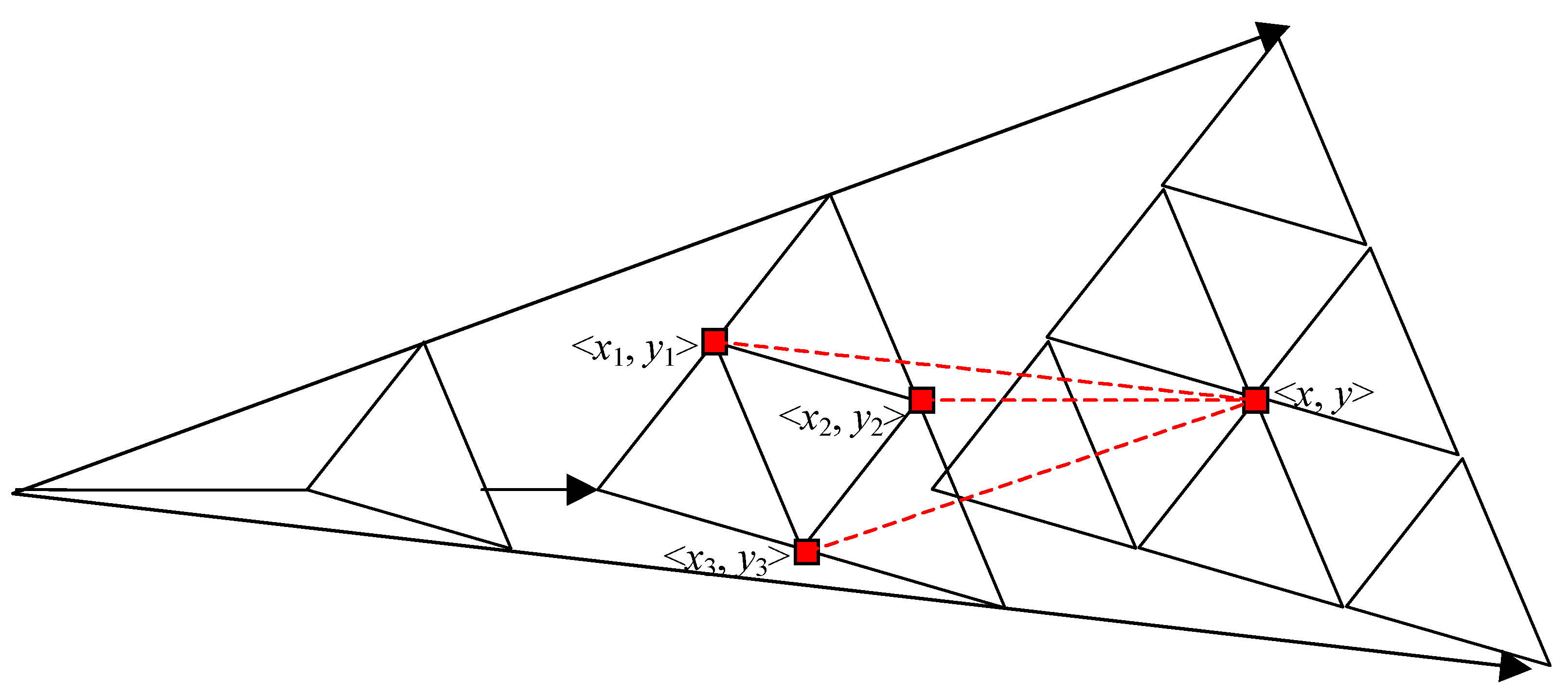
Here, we illustrate how to implement the Chen–Chung–Yang model to evaluate American-style derivatives on multiple assets. A geometrical demonstration is provided for the two-asset case as follows:
In the above demonstration, as we travel along the lattice forward, the number of nodes increases in the following geometric series: j = ( i + 1 ) ( i + 2 ) 2 ! , where i = 1 , 2 , , n as the time steps of the lattice. The general case for m number of assets is: j = 1 m ! Π k = 1 m ( i + k ) as in the following table:31
num of assetsm = 1m = 2m = 3m = m
ijjj j
0111 1
1234 5
23610 15
341020 35
n n + 1 ( n + 1 ) ( n + 2 ) 2 ! ( n + 1 ) ( n + 2 ) ( n + 3 ) 3 ! k = 1 m ( n + k ) m !
To implement the model as described in Figure A1, we index the states as follows (where the first subscript is time and the second is state):
Figure A1. A two-asset Chen–Chung–Yang Model.
Jrfm 14 00057 g0a1
[ x 01 y 01 ] [ x 11 y 11 x 12 y 12 x 13 y 13 ] [ x 21 y 21 x 22 y 22 x 23 y 23 x 24 y 24 x 25 y 25 x 26 y 26 ]
In a general case where we move from any time i to time i + 1 , state j will become < j 0 , j 1 , j 2 > as follows:
( i , j ) { ( i + 1 , j 0 ) ( i + 1 , j 1 ) ( i + 1 , j 2 )
where
j 0 = j j 1 = i ( i + 1 ) 2 + k j 2 = j 1 + 1
As i = 1 ~ n , we have:
j = { ( i 1 ) i 2 + 1 } ~ { i ( i + 1 ) 2 } k = k + 1 ( 1 ~ i )

References

  1. Boyle, Phelim P. 1988. A Lattice Framework for Option Pricing with Two State Variables. Journal of Financial And Quantitative Analysis 23: 1–12. [Google Scholar] [CrossRef]
  2. Boyle, Phelim P., Jeremy Evnine, and Stephen Gibbs. 1989. Numerical Evaluation of Multivariate Contingent Claims. The Review of Financial Studies 2: 241–50. [Google Scholar] [CrossRef]
  3. Carr, Peter. 1998. Randomizing and the American Put. Review of Financial Studies 11: 597–626. [Google Scholar] [CrossRef]
  4. Carr, Peter, Robert Jarrow, and Ravi Myneni. 2008. Alternative Characterizations of American Put Options. Financial Derivatives Pricing 2: 85–103. [Google Scholar]
  5. Chen, Ren-Raw, San-Lin Chung, and Tyler T. Yang. 2002. Option Pricing in a Multi-Asset, Complete Market Economy. The Journal of Financial and Quantitative Analysis 37: 649–66. [Google Scholar] [CrossRef] [Green Version]
  6. Cox, John C., Stephen A. Ross, and Mark Rubinstein. 1979. Option Pricing, a Simplified Approach. Journal of Financial Economics 7: 229–63. [Google Scholar] [CrossRef]
  7. Dorigo, Marco, and Luca Maria Gambardella. 1997. Ant Colony System: A Cooperative Learning Approach to the Traveling Salesman Problem. IEEE Transactions on Evolutionary Computation 1: 53–66. [Google Scholar] [CrossRef] [Green Version]
  8. Dorigo, Marco, Vittorio Maniezzo, and Alberto Colorni. 1991. Ant System: An Autocatalytic Optimizing Process. Technical Report. Milano: Politecnico di Milano Department of Electronics, pp. 91–016. [Google Scholar]
  9. Eberhart, Russell C., and James Kennedy. 1995. A New Optimizer Using Particle Swarm Theory. Paper presented at the Sixth International Symposium on Micro Machine and Human Science, Nagoya, Japan, October 4–6. [Google Scholar]
  10. Eberhart, Russell C., and Yuhui Shi. 1998. A Modified Particle Swarm Pptimizer. Paper presented at 1998 IEEE International Conference on Evolutionary Computation Proceedings, IEEE World Congress on Computational Intelligence (Cat. No.98TH8360), Anchorage, AK, USA, May 4–9. [Google Scholar]
  11. Huang, Kaihua. 2019. Particle Swarm Optimization Central Mass on Portfolio Construction. New York: Gabelli School of Business, Fordham University. [Google Scholar]
  12. Hull, John. 2015. Options, Futures and Other Derivatives. Upper Saddle River: Prentice Hall. [Google Scholar]
  13. Jamous, Razan A., Al-Aguizy Tharwat, Essam El Seidy, and Bayoumi Ibrahim Bayoumi. 2015. A New Particle Swarm with Center of Mass Optimization. International Journal of Engineering Research and Technology 4: 312–17. [Google Scholar]
  14. Kamrad, Bardia, and Peter Ritchken. 1991. Multinomial Approximating Models for Options with k State Variables. Management Science 37: 1640–52. [Google Scholar] [CrossRef]
  15. Kumar, Sajjan, Susmita Sau, Diptendu Pal, Bhimsen Tudu, Swadhin K. Mandal, and Nilanjan Chakraborty. 2013. “Parametric Performance Evaluation of Different Types of Particle Swarm Optimization Techniques Applied in Distributed Generation System. Paper presented at the International Conference on Frontiers of Intelligent Computing: Theory and Applications (FICTA), Odisa, India, January 14–16; pp. 349–56. [Google Scholar]
  16. Longstaff, Francis, and Eduardo Schwartz. 2001. Valuing American-style derivatives by Simulation. The Review of Financial Studies I 4: 113–47. [Google Scholar] [CrossRef] [Green Version]
  17. Nunes, João Pedro Vidal. 2009. Pricing American options under the constant elasticity of variance model and subject to bankruptcy. Journal of Financial and Quantitative Analysis 44: 1231–63. [Google Scholar] [CrossRef] [Green Version]
  18. Reynolds, Craig. 1987. Flocks, herds and schools: A distributed behavioral model. Paper presented the 14th Annual Conference on Computer Graphics and Interactive Techniques, Anaheim, CA, USA, July 27–31; Association for Computing Machinery. pp. 25–34. [Google Scholar]
  19. Stulz, Rene. 1982. Options on the Minimum or the Maximum of Two Risky Assets: Analysis and Applications. Journal of Financial Economics 10: 161–85. [Google Scholar] [CrossRef]
  20. Zhang, Yudong, Shuihua Wang, and Genlin Ji. 2015. A Comprehensive Survey on Particle Swarm Optimization Algorithm and Its Applications. Mathematical Problems in Engineering 2015: 38. [Google Scholar] [CrossRef] [Green Version]
1
By efficient, we refer to the balance between speed and accuracy.
2
For recent work, see Carr et al. (2008). See also Nunes (2009) for a nice review/comparison of various boundaries.
3
As a reminder, a continuation value in the option literature refers to the expected value of future maximum payoff at any given point in time. Since the continuation value is the expected future payoff, it is compared to the exercise value at the given time to see if (early) exercise is worthwhile.
4
In the case of put options, the quadratic function works very well. Yet, in other forms of payoff, Longstaff and Schwartz do not provide any guidance.
5
For example, see Carr (1998).
6
7
According to Wikipedia (footnote 6), Reynold created Boid in 1986: “Boids is an artificial life program, developed by Craig Reynolds in 1986, which simulates the flocking behaviour of birds.”
8
9
These reference birds are like “my leaders” for a given bird.
10
We ignore separation in our model because in our applications, particles can take the same coordinates (i.e., collision is allowed).
11
While this is out of the scope of this paper, we encourage the readers to view a popular YouTube clip on how drones use an artificial swarm: “Skynet’Drones Work Together for ‘Homeland Security” (https://www.youtube.com/watch?v=oDyfGM35ekc).
12
Similar to PSO, an ACO (ant colony optimization) by Dorigo et al. (1991) and ACS (ant colony system) by Dorigo and Gambardella (1997) are both based upon swarm intelligence. The first ant system was first developed by Dorigo et al. (1991) and then popularized by Dorigo and Gambardella (1997).
13
A brief analysis of the min/max option is provided in the Appendix A.
14
The reason is that as a particle is approaching the global best, the velocity should approach 0 (i.e., the particle should no longer move at the global optimum).
15
PSO can also vary in terms of parameterization such as center mass (see Jamous et al. 2015).
16
This includes quantum-behaved PSO, bare-bones PSO, chaotic PSO, and fuzzy PSO.
17
This includes von Neumann, ring, star, random, among others.
18
This is to combine PSO with genetic algorithm, simulated annealing, Tabu search, artificial immune system, ant colony algorithm, artificial bee colony, differential evolution, harmonic search, and biogeography-based optimization.
19
This includes multi-objective, constrained, discrete, and binary optimization.
20
This includes parameter selection and tuning, and convergence analysis.
21
This involves multi-core, multiprocessor, GPU, and cloud computing forms.
22
They are electrical and electronic engineering, automation control systems, communication theory, operations research, mechanical engineering, fuel and energy, medicine, chemistry, and biology.
23
Kumar et al. (2013) examines the performance of various PSO algorithms: Canonical PSO, Hierarchical PSO (HPSO), Time varying acceleration coefficient (TVAC) PSO, Self-organizing hierarchical particle swarm optimizer with time-varying acceleration coefficients (HPSO-TVAC), Stochastic inertia weight (Sto-IW) PSO, and Time varying inertia weight (TVIW) PSO have been used for comparative study. These versions of PSO vary only in parameterization.
24
See Huang (2019) for a survey.
25
Certainly, we can increase the number of periods in the binomial model to achieve more accurate American values; however, this is not our main focus.
26
Note that time step 100, or T 100 , is equal to the maturity time, which is 1 (year) in the example. Hence, T26 = 0.26 and T74 = 0.74.
27
As mentioned in footnote 25, we can increase the number of steps in the binomial model to smooth the exercise boundary further.
28
For 4 assets, it requires over 1.6 billion nodes.
29
This problem has been solved by Chen et al. (2002). Later, we adopt their model as the benchmark for options on multiple assets.
30
We assume the readers are fairly familiar with the standard binomial model of Cox et al. (1979). The notation used here is quite standard (e.g., see Hull 2015) and straightforward.
31
Note that even in the simplest independence case, the number of nodes at the time step n is (n + 1)m. For example, for three periods, a four-asset model has 256 nodes as opposed to 35 nodes in the CCY model.
Figure 1. Three major parameters in a swarm. Sources: https://en.wikipedia.org/wiki/Boids.
Jrfm 14 00057 g001
Figure 2. (a) Function (16). (b) Function (17). For an animated demonstration, see for example, https://en.wikipedia.org/wiki/Particle_swarm_optimization#/media/File:ParticleSwarmArrowsAnimation.gif.
Jrfm 14 00057 g002aJrfm 14 00057 g002bJrfm 14 00057 g002c
Figure 3. Various exercise boundaries.
Jrfm 14 00057 g003
Table 1. American put results taken from crr3d.xls. The option payoff is: max { K S } , 0 } .
stock price100
strike price100
volatility0.3
risk-free rate0.03
time to maturity1
time steps100
Monte Carlo paths10,000
Put Option
EuropeanAmerican
Black–Scholes10.3278N.A
binomial (CRR)10.298410.5917
Longstaff–Schwartz10.365610.6217
PSO-flat10.365610.5591
PSO-linear10.365610.5621
PSO-exponential10.365610.6647
PSO-piecewise10.365610.7714
PSO-piecewise(restricted)10.365610.6908
Note: Monte Carlo results are based upon 10,000 paths and 100 time steps. The Longstaff–Schwartz model (1991) uses a quadratic function in the regression. The PSO uses a swarm size of 500. The two parameters of the PSO are (Equation (12)): w = 0.5, c1 = 0.5 and c2 = 0.5. The computation stops when the improvement of the value is less than 10−6. The binomial model is from Cox et al. (1979) and is performed with 100 time steps. The performance of PSO is provided in Table 4.
Table 2. Put option on Min/Max. The option payoff is max { K max { S 1 , S 2 } , 0 } .
asset 1asset 2
price4040
volatility0.20.3
strike35
time to maturity7/12
risk free rate0.03
correlation0.5
Min/Max Option
EuropeanAmerican
BS0.1948N.A
binomial (CCY)0.18840.2557
Longstaff–Schwartz0.19740.2386
PSO-flat0.19740.2318
PSO-linear0.19740.2349
PSO-exponential0.19740.2361
PSO-piecewise0.19740.2426
PSO-piecewise(restricted)0.19740.2352
Note: Monte Carlo results are based upon 10,000 paths and 100 time steps. The Longstaff–Schwartz model (1991) uses a quadratic function in the regression. The PSO uses a swarm size of 500. The two parameters of the PSO are (Equation (12)): w = 0.5, c1 = 0.5 and c2 = 0.5. The computation stops when the improvement of the value is less than 10−6. The binomial model is Chen et al. (2002) and is performed with 100 time steps. The performance of PSO is provided in Table 4.
Table 3. Path-dependent Asian Option. Payoffs max { K S ¯ ( T 1 , T 2 ) , 0 } , where S ¯ = 1 n j = 1 n S j .
Average Option
EuropeanAmerican
Longstaff–Schwartz9.01099.2415
PSO-flat9.01099.0117
PSO-linear9.01099.0117
PSO-exponential9.01099.0117
PSO-piecewise9.01099.1925
PSO-piecewise(restricted)9.01099.1912
Note: Monte Carlo results are based upon 10,000 paths and 100 time steps. The Longstaff–Schwartz model (2001) uses a quadratic function in the regression. The PSO uses a swarm size of 500. The two parameters of the PSO are (Equation (12)): w = 0.5, c1 = 0.5 and c2 = 0.5. The computation stops when the improvement of the value is less than 10−6. The binomial model is performed with 100 time steps. The performance of PSO is provided in Table 4.
Table 4. Performance of PSO.
(A) Put Option (1-asset)
Value ($)
Seed69,90580,302824926,79596712,12881,91726,488314341,675MeanMaxMin
Swarm Size
5010.03689.700110.247010.11099.803910.158610.271210.50069.31649.41689.956210.50069.3164
10010.038810.43299.290210.015610.576010.234510.551210.25849.84049.768310.100610.57609.2902
20010.07449.77769.814910.507610.303910.632910.099910.706610.51649.841510.227610.70669.7776
50010.581110.020210.579110.745910.707410.523710.495010.697710.771410.412710.553410.771410.0202
Computation Time (seconds)
Seed69,90580,302824926,79596712,12881,91726,488314341,675MeanMaxMin
Swarm Size
5019.682918.818718.830418.571018.302118.959918.863319.274618.874319.064518.924219.682918.3022
10037.374836.921838.139736.741937.884537.110337.969337.197637.758937.740237.483938.139736.7419
20075.149275.146177.289175.034674.684975.858976.639173.807876.621373.011075.324277.289173.0110
500186.9830185.8080178.4430182.4440186.9290185.8810184.2930183.5500185.3380178.0620183.7732186.9831178.0624
(B) Min/Max Option (2-asset)
Value ($)
Seed69,90580,302824926,79596712,12881,91726,488314341,675MeanMaxMin
Swarm Size
500.22680.23580.23500.23680.23740.23470.23830.23930.22570.23530.23450.23930.2257
1000.23340.23440.23980.23790.23640.23420.23420.23810.23840.23820.23650.23980.2334
2000.23830.23800.23680.23150.23740.23350.23380.23870.24090.23200.23610.24090.2315
5000.23590.23420.23660.24120.24130.24260.24140.23920.24160.23620.23900.24260.2342
Computation Time (seconds)
Seed69,90580,302824926,79596712,12881,91726,488314341,675MeanMaxMin
Swarm Size
5010.731220.670720.598620.554920.706916.122320.682420.66496.9715320.707317.841120.70736.9715
10041.100344.562445.63441.028241.20140.791641.161440.688125.104946.883740.815646.883725.1049
20087.669473.136378.161783.915586.751573.653181.17286.279381.564940.906877.321187.669440.9068
500203.568202.788219.504229.666222.398202.404210.968203.651207.758202.525210.5230229.6660202.4040
Note: The two parameters of the PSO are (Equation (12)): w = 0.5, c1 = 0.5 and c2 = 0.5. The computation stops when the improvement of the value is less than 10−6. The Longstaff–Schwartz value is 0.2386 (Table 2). The binomial model value is 0.2557 (Table 2).
Publisher’s Note: MDPI stays neutral with regard to jurisdictional claims in published maps and institutional affiliations.