Article

Evaluation of the Accuracy of Machine Learning Predictions of the Czech Republic’s Exports to the China

School of Expertness and Valuation, Institute of Technology and Business in České Budějovice, Okružní 517/10, 370 01 Ceske Budejovice, Czech Republic
*
Author to whom correspondence should be addressed.
J. Risk Financial Manag. 2021, 14(2), 76; https://doi.org/10.3390/jrfm14020076
Submission received: 12 January 2021 / Revised: 1 February 2021 / Accepted: 3 February 2021 / Published: 10 February 2021
(This article belongs to the Special Issue Artificial Neural Networks in Business)

Abstract

:
The objective of this contribution is to predict the development of the Czech Republic’s (CR) exports to the PRC (People’s Republic of China) using ANN (artificial neural networks). To meet the objective, two research questions are formulated. The questions focus on whether growth in the CR’s exports to the PRC can be expected and whether MLP (Multi-Layer Perceptron) networks are applicable for predicting the future development of the CR’s exports to the PRC. On the basis of previously obtained historical data, ANN with the best explanatory power are generated. For the purpose specified, three experiments are carried out, the results of which are described in detail. For the first, second and third experiments, ANN for predicting the development of exports are generated on the basis of a time series with a 1-month, 5-month and 10-month time delay, respectively. The generated ANN are the MLP and regression time series neural networks. The MLP turn out to be the most efficient in predicting the future development of the CR’s exports to the PRC. They are also able to predict possible extremes. It is also determined that the USA–China trade war has significantly affected the CR’s exports to the PRC.

1. Introduction

Machine learning is a part of artificial intelligence, which can be characterized as a process of using mathematical data models through which a computer is learning without receiving direct instructions. Machine learning uses algorithms for identifying patterns in data, where the patterns are used for creating a data model able to formulate various types of predictions. The more data and experience available, the more accurate the results of machine learning prediction are (Culkin and Das 2017). Besides predicting, machine learning can currently be applied in many other aspects of today’s society, starting from autonomous vehicles to image recognition, health informatics or bioinformatics. According to Mosavi et al. (2020), due to its adaptability, machine learning is a great option for the situations when data are constantly changing, when the character of requirements or tasks is changing, or when it is not effective to program a solution. Nosratabadi et al. (2020) categorize and study machine learning in popular technologies, such as deep learning, hybrid learning models, and ensemble algorithms. The author further adds that thanks to the fast development of data, information technologies, and remarkable advance in data analysis methods, there has recently been an exponential increase in the application of machine learning in finance and economics, which, so far, have brought promising results. This is confirmed by the fact that many researchers, in their research, have dealt with machine learning models in order to apply them for solving various problems related to these fields. Interesting research was conducted by Wang and Xu (2018), who, in their study, presented a new deep learning model for investigation of car insurance frauds. Machine learning was used in research conducted by Ha and Nguyen (2016), who studied feature selection methods to help financial institutions to conduct credit risk assessment more easily. The authors focus on the most important variables and improve the accuracy of the classification in terms of assessment of credits and customers. Das and Mishra (2019) use a multilayer deep neural network (MDNN) optimized by Adam Optimizer (AO) for designing an advanced model for planning, analysis, and predicting the value of shares in order to find patterns between values of shares. From a large number of studies on the application of machine learning, it is worth mentioning the research by Lahmiri and Bekiros (2019), who applied the methods of deep learning for predicting the price of cryptocurrencies including bitcoin, digital cash, and ripple, and compared the prediction performance of LSTM (Long Short-Term Memory) and GRNN (Generalized Regression Neural Network). Their findings show that the performance of the LSTM model is better than the performance of GRNN.
This contribution deals mainly with the process of predicting export using machine learning. Specifically, it is focused on predicting the development of the Czech Republic’s (CR) exports to the PRC (People’s Republic of China) using ANN (artificial neural networks) of the MLP (Multi-Layer Perceptron) type. Although there are many studies dealing with predicting using machine learning, and despite the fact that MLP is considered a well-known and a widely applied machine learning method, its application for predicting exports has not been investigated sufficiently. This fact is thus perceived as a certain limitation in research.
This contribution brings novelty and promising results in the area of predicting exports using machine learning, or using MLP networks. This research has made it possible to find out whether MLP are a suitable tool that can be used for predicting foreign trade and how accurate they are. An accurate prediction of financial and economic data is of great importance, especially for many research workers and entities with decision-making power. These include, for example, policy makers, who, based on the correct prediction of these data, will be able to propose and implement measures for an expected financial crisis. To meet the objective of this contribution, two research questions (RQ) have been formulated:
  • RQ1: Can there be expected a growth in the CR’s exports to the PRC?
  • RQ2: Are MLP networks applicable for predicting the future development of the CR’s exports to the PRC?
The structure of this contribution is as follows: The introductory part above specifies the trade relationship between the CR and the PRC. Furthermore, the text mainly focuses on export and import studies, whereby a major part of the text deals with research into methods and models of machine learning that are able to predict the aforementioned indicators. The following part of the text presents the methods and data used for achieving the set objective of the contribution, i.e., machine learning predictions of the CR’s exports to the PRC. In the results section, regression by means of neural structures is carried out. Three experiments are presented, for which three sets of ANN were generated, with different time series lags of 1, 5 and 10 months, respectively. In the conclusions, the results of these three experiments are compared to determine whether the selected method of machine learning is applicable in terms of the research focus. In addition, the direction of further research based on the conclusions of this contribution are outlined.

2. Literature Research

The CR is a country characterised by high and growing intra-industry trade. Most recently, there has been an increase in intra-industry trade with China (Wysokińska 2010). According to Humlerova (2018), China has been the CR’s fourth largest trading partner and second largest importer since 2006. On the other hand, China is the 18th largest export market for the CR. It is estimated that there has been a 68% increase in the CR’s exports to China in the last five years. Between 2007 and 2011, Czech exports to China experienced a significant surge. This increase has made China a leading trading partner for the CR. Overall, the CR’s total exports to other countries of the world grew significantly in 2013 and 2014 (Povolna and Svarcova 2017). Similar trends were observed by Koncikova (2013). Havrlant and Husek (2011) focused on analysing factors that influence the CR’s exports. Factors influencing the volume of exports of any state usually include foreign demand, domestic and foreign price levels, and exchange rates. According to Ogbuabor (2019), the economy of the CR has been strongly influenced by neighbouring countries, such as Germany, Austria and Poland, since the recession in the years 2012/2013. In recent years, however, the USA has also begun to have an effect on the economy of the CR. This is reflected in the imports and exports between the CR and other states the country maintains trade relations with. According to Rojicek (2010), the CR is strongly dependent on good export performance. The process of globalization, therefore, has a significant impact on the Czech economy. The export performance of the CR as such is determined by its geographical location, qualified and cheap workforce, and also its membership in the EU. The radical changes in the trading relationship between the two partners left researchers with no option but to investigate machine learning prediction methods for predicting the development of the CR’s exports to the PRC, and to compare its advantages and disadvantages with other methods.
An analysis by Fojtikova (2018) confirmed a significant increase in market share for China in the steel industry in comparison with the CR, which, as Fojtikova (2018) believes, has had a negative impact on the Czech steel industry. The application of the Grubel–Lloyd index to calculate the level of intra-industry trade between the CR and China confirms the ongoing trade deficit, as well as the significant growth of imports from the PRC (Fojtikova and Meng 2018). According to Yin et al. (2017), the total volume of trade of a country is an important indicator for evaluating the international trade conditions. By using the Grey Wave (GW) prediction model with the Hodrick–Prescott filter, the researchers predicted the volume of Chinese trade. One of the advantages of predicting the volume of trade is that it helps enterprises to arrange efficient production and support international trade sustainability. According to Wu et al. (2009), the import of some commodities is risky for the PRC due to the different origin of prices. For example, the import of oil is a specific problem due to its constantly changing value. The risk resulting from the import of oil can be eliminated by importing oil-based products in order to reduce the volume of oil imports. The constant growth of the automotive industry and other industries where energy demands have grown goes some way to explain this phenomenon (Zhao and Wu 2007). According to Wu et al. (2017), commodities imported to the PRC from other states have an additional effect on domestic product rather than a supplementary one. The imported commodities, however, may cause inflation problems in the PRC; the PRC government should, therefore, focus on supporting domestic production in order to eliminate this risk. As Allen and Den (2014) state, the demand for the import of non-renewable resources to the PRC increases at cyclical intervals during boom periods in a specific sector of the PRC’s economy. During the boom periods, the volume of demand changes and at the end of the period, it stabilizes at its normal values. This is also related to the fluctuations in prices of these imported non-renewable resources. Nevertheless, it has never been recorded that the PRC’s demand for renewable resources would completely deplete the reserves of non-renewable resources of any importing country. Laio et al. (2020) claim that in addition to the import of resources and goods, the PRC should also be interested in importing new technologies and innovations in order to improve the quality of life of its citizens.
How is it generally best to analyze and predict trade balance time series? A comparison of econometric models and ANN by Zhang et al. (2019) showed that the application of time series data enables econometric forecasting models to provide better predictions than ANN algorithms. However, ANN algorithms produce fewer errors and a higher matching rate than econometric models using long term data. Nevertheless, according to Zhang et al. (2019), generalizing autoregressive heteroskedasticity models and back propagation neural networks produces the best predictions. Sokolov-Mladenovic et al. (2016) also applied ANN with back propagation learning and extreme learning machine (ELM) algorithms to predict GDP growth rates. They concluded that ELM can be applied effectively for forecasting GDP growth rates. Production and exports are directly related to fluctuations in GDP and the economic cycle. Janda et al. (2013) conclude that traditional prediction methods, which include all observations into one model, do not provide significant results. However, higher GDP, shorter distance, or lower political risk have a positive impact on Czech exports.
By considering different learning algorithms such as support vector machines (SVM), Parzen windows, and Fisher discriminant analysis, Zlicar and Cousins (2018) concluded that sequential Parzen windows were capable of outperforming the other models. Lahmiri (2014) used the entropy statistics and polynomial-based kernel SVM to predict the future fluctuations of stock prices. In addition to the model presented by Lahmiri (2014), Land et al. (2007) pointed to the fact that SVM regression algorithms can be trained in real time and have the theoretical capability of achieving the global minimum. Chou (2010) used a comparison of mixed fuzzy expert system and regression models, and traditional and non-traditional linear regression models, for predicting imports. On the basis of the results, the author concluded that mixed fuzzy expert system and regression displays higher prediction accuracy. Many other researchers, such as Sidehabi et al. (2016) and Polak (2019), used the Adaptive Spline Threshold Autoregression (ASTAR) statistical method, and created a commercial risk assessment model specifically for Czech companies that export goods and technologies to China in order to help them determine future export volumes to the PRC.
The research conducted by Hushani (2019) compared four predictive models for stock market prediction and trading: the Autoregressive Integrated Moving Average (ARIMA), the model of Vector Autoregression (VAR), the model of LSTM, and the Nonlinear Autoregressive Exogenous model (NARX). In addition, the objective of the research was to develop a new profitable business strategy. It followed from the research results that the NARX model provides accurate short-term predictions, but long-term predictions are unsuccessful. The VAR model can create a good trend curve required for trading. Profitable business strategy can, thus, combine predictive modelling of machine learning and technical analysis.
The research by Lu et al. (2020) aimed to predict carbon prices and trading volumes on eight Chinese markets by means of six models of machine learning: XGBoost, Radio Frequency (RF), Gray Wolf Optimization-Kernel-Based Nonlinear Arps (GWO-KNEA), Particle Swarm Optimization-Support Vector Machine (PSO-SVM), Simulated Annealing-Fruit Fly Optimization Algorithm-Support Vector Machine (SA-FFOA-SVM), and Radial Basis Functions Neural Networks (RBFNN). In addition, the authors used an advanced method of data noise reduction, i.e., the Complete Ensemble Empirical Mode Decomposition with Adaptive Noise (CEEMDAN). The prediction results show that CEEMDAN-GWO-KNEA and CEEMDAN-RBFNN were more competitive in predicting carbon prices and trading volumes due to their high performance in many datasets. The average accuracy of CEEMDAN-RBFNN and CEEMDAN-GWO-KNEA in predicting carbon prices was 98.40%, or 97.89%. The predictive stability of each model, in various application scenarios, was also discussed. The results showed that high prediction accuracy does not correspond to better stability prediction, but CEEMDAN-RBFNN and CEEMDAN-GWO-KNEA can still guarantee high stability in most datasets.
Nabipour et al. (2020b) aimed to compare the predictive performance of nine models of machine learning (Decision Tree, Random Forest, Adaboost, XGBoost, SVC—Support Vector Classifier, Naïve Bayes, KNN—K-Nearest Neighbors, Logistic Regression, and ANN) and two deep learning methods (RNN—Recurrent Neural Network, and LSTM) for predicting developments in the stock market. The authors selected (from the Tehran Stock Exchange) a total of four groups of stock markets: diversified financials, oil, non-metallic minerals, and base metals. The study included two different approaches to inputs—continuous data and binary data—and each model was evaluated using three metrics. The results showed that compared to continuous data, the use of binary data significantly improved the performance of the models. Furthermore, it was found that within both approaches, deep learning algorithms showed better performance, especially the RNN and LSTM models, which significantly outperformed the other models.
Similar research was conducted by Nabipour et al. (2020a), who applied models based on trees (Decision Tree, Bagging, Random Forest, Adaboost, Gradient Boosting, and XGBoost) and neural network models (ANN, RNN, and LSTM) to accurately predict the values of four groups of stock markets within the Tehran Stock Exchange. The predictions were created for 1, 2, 5, 10, 15, 20, and 30 days in advance. Based on the results, the authors concluded that both tree-based and deep learning algorithms showed remarkable potential for predicting the values on the Tehran Stock Exchange. The best model turned out to be the LSTM model, which showed the smallest error and the best adaptability.
Sebastião and Godinho (2021) agree that the machine learning models provide excellent techniques for examining predictions, specifically the predictions of cryptocurrencies and proposing profitable business strategies on these types of markets even under unfavourable conditions. The authors dealt with predictions of three main cryptocurrencies (bitcoin, ethereum, and litecoin) and the profitability of business strategies proposed on the basis of machine learning techniques (e.g., linear models, random forests, and support vector machines).
It follows from above that researchers have recently been increasingly interested in the application of machine learning methods, or ANN. There have also been more publications dealing with their description and principles. A relatively clear description of ANN is provided, e.g., by Klieštik (2013), who considers them to be computational models inspired by biological neural networks, especially the behaviour of neurons. Hogenboom et al. (2015) describe ANN as a flexible, non-parametrical model tool based on historical data and the ability to make predictions for the future. Horák and Krulický (2019) state that ANN are a highly efficient method for data collecting, analysis, and prediction; therefore, they may be applied for solving complex problems, difficult situations including various predictions. They are applied mainly for regression, classification, or cluster analysis. Their advantages include the ability to work with big data, the ability to learn, easy applicability of the network obtained or accuracy of results. On the other hand, their disadvantage is in the method of creating individual models of ANN (Rowland and Vrbka 2016).
The most widely used and very popular neural networks include MLP, which is used also for the purposes of this research. MLP networks are so-called feedforward ANN and consist of three main components: one input layer, one or more hidden layers, and one output layer, where the input layer accepts the values of predictive variables presented in the network (e.g., financial variables), while the output layer represents the expected output (e.g., the prediction of a company’s performance) (Ecer et al. 2020). Pinter et al. (2020) further add that for the training process, MLP use the backpropagation algorithm, which is the supervised learning of ANN by means of gradient descent, where the perceptron models the output on the basis of its weights and non-linear activation functions. According to Ramchoun et al. (2016), the popularity of MLP has become more popular recently thanks to its robustness and relatively good performance. This is confirmed by Kiranyaz et al. (2009), who also present several comparative studies, where MLP models outperform other models. Ecer (2013) adds that MLP networks are well suited for the purposes of various types of predictions.
As an example, the work of Vrbka and Vochozka (2020) can be mentioned, in which this method was used to handle fluctuations caused by seasonality in predicting the development of the PRC–USA exports and imports. On the basis of their research, it was found that parameters such as seasonality or data analysis based on monthly intervals is the right way to ensure that ANN provide accurate prediction results. Vochozka and Rowland (2020) also tried to predict the development of the balance of trade between the CR and the PRC using ANN by means of MLP and radial basis function networks (RBF), whereby seasonal fluctuations were also taken into consideration. Within this context, MLP networks appeared to produce better prediction results. Krulicky and Brabenec (2020) compared the possibilities of the predictions of the CR’s imports to the PRC on the basis of regression analysis and ANN based on monthly data from the years 2000–2018. ANN were evaluated as more efficient in their predictions. Machova and Marecek (2020) dealt with the PRC’s imports to the CR from the perspective of sanctions imposed on international trade between the PRC and the USA. The analysis of data with regard to the development of exports and imports between the PRC and the USA, as well as between the PRC and the CR, showed that the imposed sanctions had had no negative impact on the PRC’s exports to the CR.
On the basis of current evidence, researchers state that in the past, many conventional methods were used to predict the volume of international exports. Investors applied mathematical and statistical tools for technical and quantitative financial trading analysis. In recent years, new techniques such as machine learning and datamining have appeared to replace traditional approaches. Apart from ANN and SVM, other models have also proven to have practical applications (Gerlein et al. 2016). This is supported by Castillo and Melin (1997), who consider artificial intelligence methods to be the best instruments for modelling and generating simulations of international trade. These instruments can be developed to obtain the best mathematical models for specific circumstances.
In conclusion, in today’s world, the use of machine learning to predict exports is vital. The research presented here therefore focuses on investigating machine learning predictions of the CR’s exports to the PRC. A number of traditional and more recent prediction methods are highlighted in this review. The reviewed literature indicates that there are advantages and disadvantages to the application of artificial intelligent machine learning techniques when compared with other tools. With access to large data sets, ANN tools are capable of working with big data; however, there is a high level of error susceptibility. Current research supports the use of ANN.

3. Materials and Methods

Mutual trade relations between the United States of America and the PRC have recently been rather unstable. It can even be said that a trade war has broken out between both countries, with each slapping duties on one another’s imported goods. The situation was escalated by the USA in an attempt to address the trade imbalance. After some time, China responded in kind. The mutual trade relationship between the USA and the PRC is clearly described in Appendix A. However, this situation not only influenced trade between the two powers, but also had far reaching consequences for the whole world. The PRC, which produces a large number of different products, has to constantly seek new markets for them. The country has, therefore, sought to boost its exports to countries where its products can be sold for reasonable prices and where the respective products are not subject to import duties. However, the question is whether the PRC will allow (over time) its new partners to import to the PRC. Within this context, the trade war will also affect trade between the CR and the PRC. The question, therefore, arises as to whether it will always be possible to predict the future development of mutual trade; i.e., imports and exports between the CR and the PRC. This contribution focuses on the accuracy of predicting the CR’s exports to the PRC using machine learning prediction.
The data set below demonstrates the course of the time series at monthly intervals from January 2000 to June 2019. The course of the time series is presented in Figure 1.
The figure shows the dramatic fluctuations for the individual years during the monitored period. However, the question is whether regular seasonal fluctuations need to be taken into consideration, or whether these fluctuations are a unique phenomenon caused by the fragility of the long-term trade relationships between Czech and Chinese business partners. What is also evident is the considerable growth in the value of exported Czech goods to the PRC. The lowest volume of exports amounted to less than USD 2.5 million/month, while the highest volume exceeded USD 206 million/month during the monitored period, which is more than 84-times more. The lowest value was observed in July 2000. On the other hand, exports from the CR to the PRC reached their highest value in October 2018. From then, up to the end of the monitored period, exports fell to nearly USD 184 million in June 2019. The question is whether seasonal fluctuations were the only cause. Table 1 presents the basic statistical characteristics of the data set.
Regression using neural structures is performed and MLP generated. Three data sets of ANN are subsequently created based on the time delay of the time series:
  • Time series delay of 1 month;
  • Time series delay of 5 months;
  • Time series delay of 10 months.
The time series delay consists of a set of data from which a following value is calculated (i.e., in the first case from the value of one previous month; in the second case from the previous five values; in the third case from the previous 10 values). Longer delays in time series may result in averaged values. On the other hand, shorter delays in time series may cause extreme fluctuations in equalizing the time series. Delays in time series cannot, therefore, be used for the analysis of seasonal fluctuations in time series, as they only refer to the complexity of the predicted values and the number of inputs for such a calculation. Each time series delay requires a more complex artificial neural structure, neurons in the input layer in particular (for Experiments 1, 2 and 3, the input layer contained 3, 15 and 30 neurons, respectively). The other parameters for the experiments are identical.
Seasonal fluctuations may be analysed by determining the trend of the time series development; i.e., the relevant setting of the input variables. Within this context, time is used as a continuous independent variable. Seasonal fluctuations are represented by a categorical variable of the month and year in which the value was observed. In this way, possible monthly seasonal time series fluctuations are, therefore, dealt with. The general trend of the time series is also taken into consideration. The dependent variable is the CR’s exports to the PRC.
The time series is divided into three data sets—training, testing and validation. The first group contains 70% of the input data. This data set is also used to generate the neural structures. The remaining two data sets contain 15% of the input data each. Both groups are used to verify the reliability of the identified neural structure, i.e., the identified model. A total of 10,000 neural networks are generated, out of which the five with the best characteristics are retained. The hidden layer contains from 2 to 12 neurons in the case of Experiment 1, and 15 neurons for Experiments 2 and 3. The distribution functions in the hidden and output layers are as follows:
  • Linear;
  • Logistic;
  • Atanh;
  • Exponential;
  • Sine.
The other parameters remain default (according to the ANN tool). The expected outcomes are as follows:
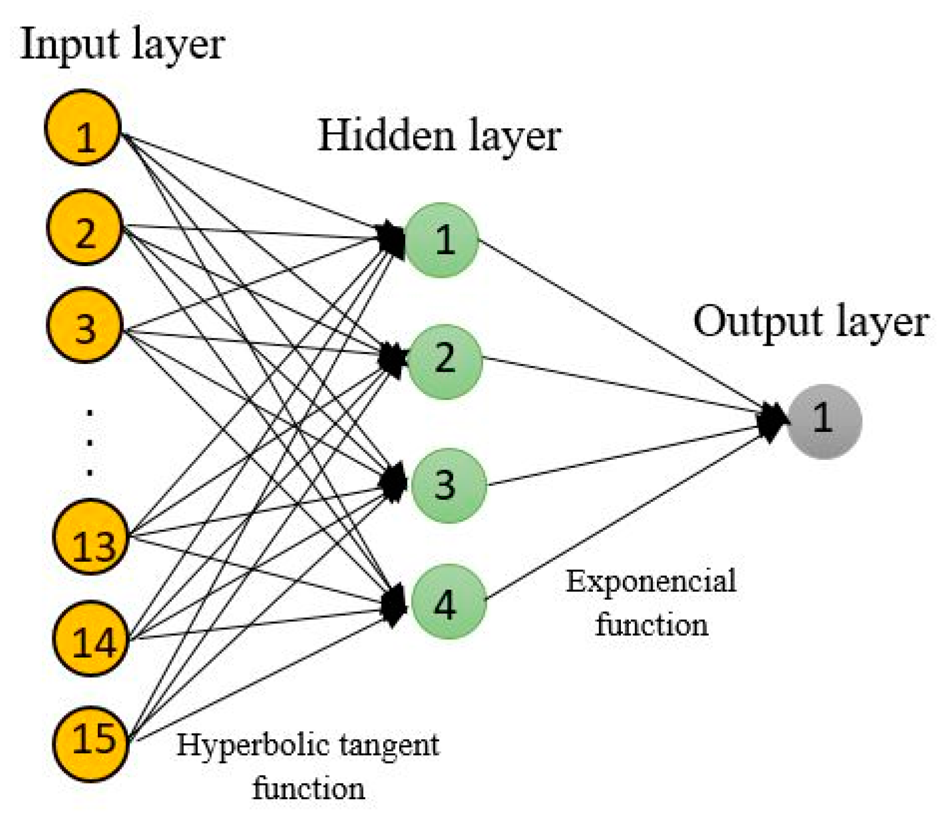
  • The overview of the retained networks always contains the structures of the five retained neural networks, the performance of the data sets, errors, the error function, and the activation function of the input and output layers of the neural network.
  • Correlation coefficients that characterise the network performance in individual data subsets.
  • Basic statistics of equalized time series.
  • A diagram of equalized time series.
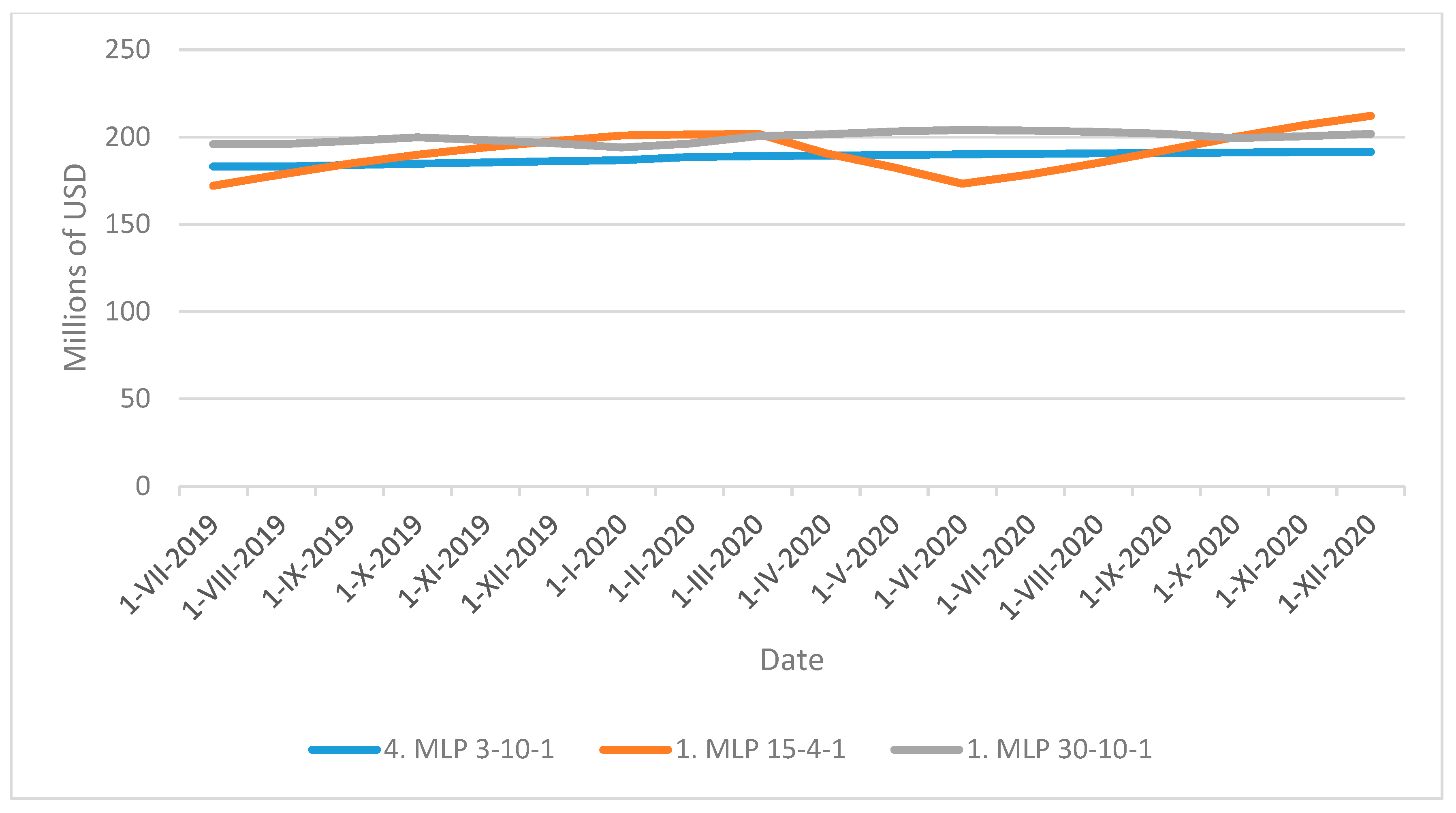
  • Predicted values from July 2019 to December 2020.
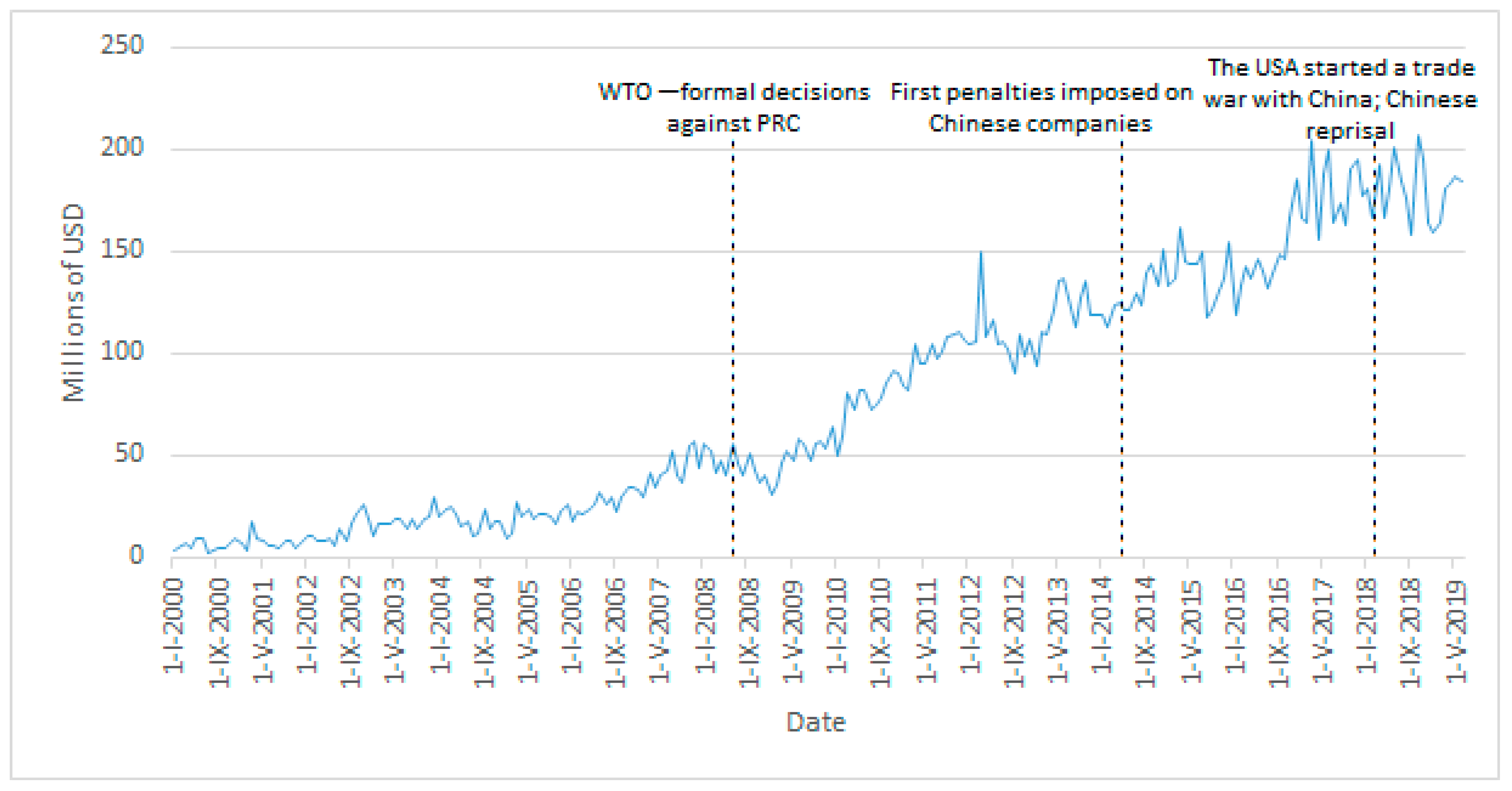
  • A diagram of the development of an actual time series related to the predictions, i.e., possible development of the time series from January 2000 to December 2020.
In the conclusions, the results of the three experiments are compared and it is determined whether the proposed method of machine learning prediction is efficient, and which delay is the closest to the positive result.

4. Results

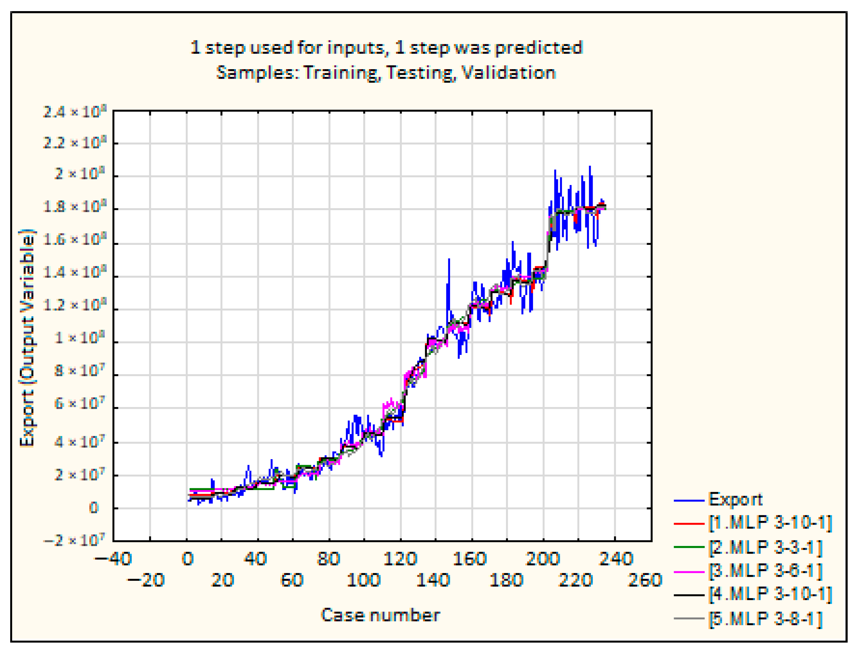
4.1. Experiment 1 (Time Series Delay of 1 Month)

Table 2 shows an overview of the retained neural networks from Experiment 1.
It follows from the table that the retained neural networks contained between 3 and 10 neurons in the hidden layer. The input layer of neural networks always contained three neurons (the date, month and year when the values were measured). For the activation of the hidden layer, the logistic function and hyperbolic tangent were used. The output layer was activated using the exponential and logistic functions. The performance of neural networks is also very important and is expressed by a correlation coefficient. The correlation coefficient in all the data sets was very high. In the case of the training data set, the correlation coefficient achieved the value of 0.99. As applied by analogy, the testing data set showed a high correlation coefficient for the retained neural networks—always exceeding 0.99. In the case of the validation data set, its values also achieved the value of 0.99, which indicates almost direct dependence. The neural structures should, therefore, be able to predict the future development of the monitored time series in a relatively accurate way. However, they must not suffer from overfitting. The errors identified were found to be acceptable on the basis of the method of least squares.
Figure 2 presents a comparison of the actual trend of the time series and the equalized time series.
Figure 2 shows that all equalized time series reflect the apparent trend of the actual development of the CR’s exports to the PRC. Nevertheless, what cannot be precisely observed are the endings of some local extremes throughout the time series. The biggest issues regarding the equalized time series appear approximately from the 200th case, which corresponds to the period from July 2016 to June 2019.
In order to determine whether the networks are applicable, their predictive ability must be examined. For that reason, the development of the CR’s exports to the PRC from July 2019 to December 2020 was predicted. The relevant data are presented in Table 3.
It is apparent that the third network (MLP 3-6-1) predicts the future development of the monitored variable in a very inaccurate way. It shows a sharp decrease in exports and a low constant value, which is very unlikely. It is evident that the third retained neural network suffers from overfitting. The other neural networks showed only slight differences. In order to choose the best neural network, the time series and predicted development are presented in Figure 3.
From the figure, it is evident that the predictions of the other networks are also inaccurate; they were not able to identify (if relevant for a specific network) seasonal fluctuations. The question is whether they suffer from overfitting. Although this is very unlikely, the results are not very accurate. It was, therefore, necessary to choose one of the remaining neural networks to make a more detailed comparison. Taking into consideration the statistics for the equalized time series (Appendix B), it was concluded that the most successful and accurate neural network was the fourth (MLP 3-10-1).

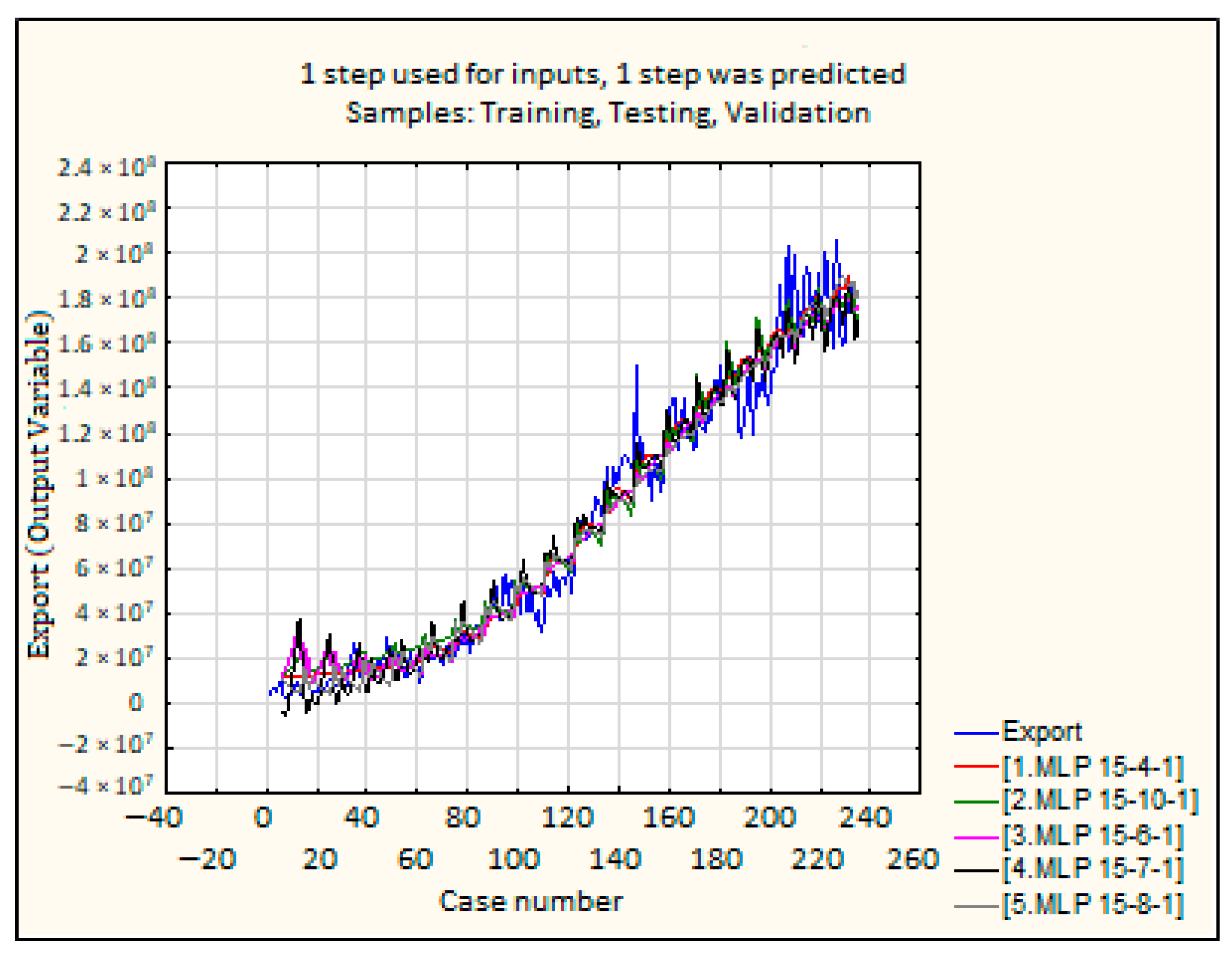
4.2. Experiment 2 (Time Series Delay of 5 Months)

A total of 10,000 ANN were generated within the equalization of the export time series; the five with the best characteristics were retained (see Table 4).
In the case of exports, the input layer contained 15 neurons. The table indicates that those neural networks containing 4–10 neurons in the hidden layer were retained. The hyperbolic tangent and sine functions were used for the activation of the hidden layer. The output layer was activated using the exponential, sine, and identity functions. The performance of the ANN, as expressed by the correlation coefficient, exceeded 0.97 in the case of the training data set, 0.98 in the case of the testing data set (in the case of second MLP 15-10-1, it even exceeded 0.99), and 0.98 in the case of the validation data set. All these cases indicate a direct dependence. Based on this parameter, it can be concluded that the networks (if not overfitted) are able to predict the future development of the CR’s exports to the PRC very accurately (as they effectively equalize the time series from the past). The method of least squares was used for calculating the error. Although the export values of the calculated error were relatively significant, this error is considered acceptable in view of the extent of the individual values and the necessity of considering the USD parameter.
Figure 4 shows a comparison of the actual trend of the time series and the equalized time series.
Figure 4 shows that all equalized time series are able to capture the trend of the actual development of the CR’s exports to the PRC very well. As a result of the time series being strongly disorganized, the models cannot identify all local extremes including, e.g., the last quarter of the monitored period when the fluctuations seem rather extreme. Despite this fact, the parameters of the generated neural structures enable a good quality prediction to be made for the monitored time series (although they cannot fully capture the extremes of the time series, they adequately respond to neural network fluctuations).
As was the case for Experiment 1, the focus is on the predictive ability of the neural networks with regard to the development of the variable. The data for the predicted development of the CR’s exports to the PRC from July 2019 to December 2020 are presented in Table 5.
The data presented in the table show that none of the neural networks suffers from overfitting. The prediction made by the retained neural networks should, therefore, be applicable. In order to choose the most suitable structure to predict the CR’s exports to the PRC, a diagram of the predicted trend (Figure 5) was created.
Based on the comparison, it can be concluded (in view of the statistical table in Appendix C) that the first network (MLP 15-4-1) provides the most accurate prediction.

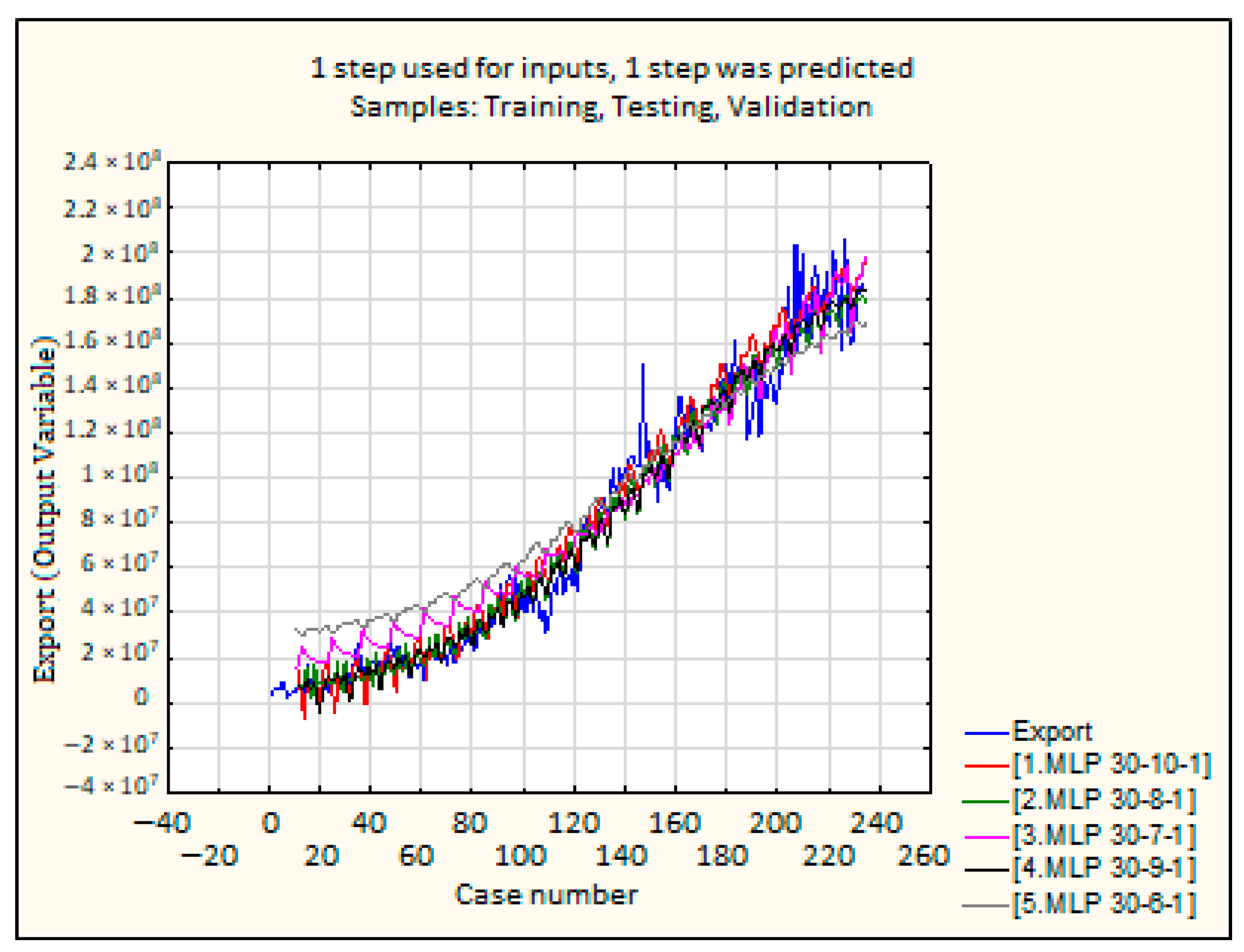
4.3. Experiment 3 (Time Series Delay of 10 Months)

In Experiment 3, 10,000 ANN were generated, out of which the five with the best characteristics were retained (see Table 6).
The results of this experiment showed 30 neurons in the input layer (date, month and 10-month delay). The table shows that those neural networks containing 6–10 neurons in the hidden layer were retained. To activate the hidden layer, the sine and logistic functions were used. The output layer was activated using the sine, exponential, logistic and hyperbolic tangent functions. The correlation coefficient for the neural networks achieved very high values, exceeding 0.97 for all data sets. This proves a high degree of direct dependence. The method of least squares was used for calculating the error. In all cases, no major error was found, which means that the quality and accuracy of the time series predictions is very good.
Figure 6 provides a comparison of the trend of the actual time series with the equalized time series.
It follows from Figure 6 that all the equalized time series are able to identify the dominant trend of the actual development of the CR’s exports to the PRC very well. In fact, some of the neural networks are able to detect most of the local extremes in the monitored time series. The fifth (MLP 30-6-1) is the most interesting; this network seems slightly turned in its centre. For the first half, the course of the equalized time series is above the actual development, but for the second half below the actual development. Although this network shows very good overall parameters, the equalized time series is quite inaccurate. What is also interesting is the third equalized time series (MLP 30-7-1), which also appears to be turned in relation to reality, yet less intensively.
As was the case in the previous two experiments, the focus is on the predictive ability of the neural networks with regard to the development of the variable. The data for the predicted development of the CR’s exports to the PRC from July 2019 to December 2020 are presented in Table 7.
As previously stated, the equalized time series are very similar to one another. However, the table indicates that some of the neural networks suffer from overfitting, which is also demonstrated in Figure 7.
The figure shows that the third network (MLP 30-7-1) suffers from overfitting, so it can be excluded from the experiment. Based on the comparison of the remaining three neural networks (according to the trend and the characteristics of all the networks), it can be concluded that the first network (MLP 30-10-1) provides the most accurate prediction of the future development (in view of the statistical table in Appendix D).

5. Discussion

Three experiments were carried out as part of the research. The development of the time series of the CR’s exports to the PRC was analysed. The way in which MLP are able to equalize time series was observed, as was the development of the variable within the context of the trade war between two global powers. For each experiment, 10,000 ANN were generated, out of which the five best structures were retained. It became apparent that some suffered from overfitting, in particular in Experiments 1 and 2. However, the other retained neural networks were applicable for predicting the future development of the CR’s exports to the PRC.
In all cases, the networks’ performance was high and the error acceptable. The best network from each experiment was determined and subsequently subjected to further analysis (see Table 8).
Table 8 shows the differences between the individual neural networks. It is evident that the differences are insignificant (within the context of the overall development of the monitored time series). This situation is more accurately shown in Figure 8.
The neural network from the first experiment was only formally implemented as it was unable to capture the seasonal fluctuations in the observed time series. Nevertheless, the network retained from Experiment 3 shows almost identical parameters to the network from Experiment 1. Their curves are concurrent. The difference in the predicted value throughout the observed period equals roughly USD 10 million. The network retained from Experiment 3 can, therefore, be excluded from the analysis. The focus is therefore on the first retained network from Experiment 2 (MLP 15-4-1). The structure was able to capture seasonal fluctuations, which appear mostly in July 2019 and June 2020. The question is whether it accurately reflects the previous trend of the analysed time series. On the whole, it can be said that it is indeed the closest to reality. What is evident is that the time series delay of 5 months was highly useful in creating and predicting the network, which resulted in a more accurate prediction. The structure of the best network (MLP 15-4-1 from Experiment 2) is shown in Figure 9.
On the basis of the above results and their discussion, it is possible to answer the research questions.
  • RQ1: Can there be expected a growth in the CR’s exports to the PRC?
The prediction made by neural networks clearly shows that there will be no increase in the CR’s exports to the PRC in the near future. Rather, a decrease of approximately 10% can be expected. The future development is determined by several factors that often have contradictory effects. In discussion of the response to the research questions, only two of these factors are mentioned: the mutual sanctions of the USA and the PRC, and the ability of the CR to secure the increase in the export to the PRC. The mutual USA–PRC balance of trade shows much higher PRC export to the USA. After imposing mutual sanctions, both countries need to find new markets for many commodities. If they fail, there will be a surplus of specific products on the market. This will first cause the decrease in the price of such products; this will reduce the producers’ incomes and creates pressure on such companies to leave the sector. To a certain extent, this will cause the market restructuring and arrival of new companies in sectors that show profit in the long run (the product that the PRC imports and is able to manufacture technologically). Chinese consumers thus start to buy larger volumes of domestic products, which results in the reduction in imports even from the CR.
The CR’s exports to the PRC consists mainly of machinery and transport vehicles, industrial and consumer goods, mainly motor vehicle components, pumps, distributors, telephones, circuits, toys, prams, or tyres (according to BusinessInfo.cz 2019). Czech companies interested in exporting their products to the PRC face a number of problems. There are administrative barriers to exporting to the PRC, fierce competition of Chinese companies on Chinese market, and logistic problems related to the transportation of products over long distances. Another problem to mention is often the inability of Czech companies to produce the required quantity of product in a specified period of time (for Czech companies often have to face the problem of their limited production capacity).
To sum up, Czech companies are able to export to the PRC certain volume of their production, and it would be difficult for them to increase this volume. The situation in the world market, however, would have rather undesirable effect for the CR, as it will reduce the CR’s exports to the PRC. Neural networks predict a decrease in the CR’s exports to the PRC equal or higher than 10%.
  • RQ2: Are MLP networks applicable for predicting the future development of the CR’s exports to the PRC?
The applicability of neural networks for smoothing the time series and subsequent prediction is given by three main factors: the performance of neural network (measured by correlation coefficient), the ability to smooth local extrema of time series, economic justification of the prediction of the time series future development. Time series smoothing was carried out as an experiment in order to determine the volume of the past data on the development of the time series for predicting. It turned out that the volume of the past data has an effect on predicting, yet not significant. The performance of all networks significantly exceeds 0.95. The graphical representation shows that smoothed time series are able to copy the local extremes of the actual CR’s exports to the PRC. Neural networks did not suffer from overfitting and are relatively easy to interpret in economic terms, which was confirmed by the answer to the RQ1.
It can thus be concluded that MLP networks and the created model are able to smooth the actual trend of the time series as well as predict the future development of the CR’s exports to the PRC.
In terms of the results of research conducted by other authors dealing with similar issues, reference can be made to, for example, Bartl and Krummaker (2020), who focused on the evaluation of four methods of machine learning in terms of their ability to accurately predict export credit financial requirements. Specifically, it included the methods of decision trees (DT), random forests (RF), ANN, and probabilistic neural networks (PNN). The results of their research indicate that all machine learning methods achieved relatively good prediction results. From the four aforementioned techniques, the decision trees method appeared to be the best one, as it converted its verification performance into the testing performance most reliably. Li et al. (2008) also dealt with the prediction of exports, specifically exports of Taiwanese polyester fibre, by means of machine learning methods with small datasets. For this purpose, the authors used the GIKDE (General Intervalized Kerned Density Estimator) method, which represents a new method for predicting future exports on the basis of small data sets. The application of this method enables more accurate predictions to be obtained, which allows managers to create plans for products, capacity and markets. The objective of the research by Rousek and Marecek (2019) was to propose a methodology for considering seasonal fluctuations in time series equalization by means of ANN on the example of US exports to the PRC. The authors used two types of neural networks and two variants of input data sets for their predictions. In the second variant, seasonal fluctuations are represented by a categorical variable. The research results indicated that all the retained neural structures were applicable; however, the retained MLP networks of variant B achieved better results. It has also been shown that ANN can be used for predicting the efficiency of export development with a high level of accuracy. It is worth mentioning here is the research conducted by Zhang (2016), who used six different input variables and China’s overall exports as an output variable for creating BP neural networks able to predict the overall exports of the country. For testing the BP model’s accuracy, the Nash–Sutcliffe efficiency coefficient (NSC) was introduced; the model was found to be highly accurate (NSC > 0.9957). Ozbek et al. (2011) used ANN and the autoregressive integrated model of moving averages to predict the export of jeans from Turkey. The research results showed that ANN models provide more accurate predictions than ARIMA models.

6. Conclusions

The objective of this article was to predict the development of the CR’s exports to the PRC using machine learning prediction. It can be stated that the objective of the article was achieved. The answers correspond to the answers to the formulated research questions. The answer to RQ1—“Can there be expected a growth in the CR’s exports to the PRC?”—can be summed up as follows:
Mutual sanctions between the USA and the PRC have significantly influenced exports from the CR to the PRC. The evidence shows a significant drop (over 10%). Mutual sanctions also affected the results produced by the machine learning prediction method. Due to rapid developments, some networks suffered from overfitting; others predicted the future development of exports very inaccurately. However, it can be argued that for this time series research, the overfitting and inaccuracies were caused by the intensifying trade war between the USA and the PRC and its dramatic impact on the CR’s exports to the PRC. The prediction shows that there will be no increase in the CR’s exports to the PRC in the near future. Rather, approximately a 10% decrease can be expected. The future development, however, is determined by several factors that have been analysed in the Discussion section and often appear to have a contradictory effect.
The answer to the RQ2—“Are MLP networks applicable for predicting the future development of the CR’s exports to the PRC?”—can be summed up as follows:
  • MLP appear to be a useful tool for predicting the development of exports from the CR to the PRC using machine learning prediction.
  • MLP networks are able to capture not only the trend throughout the time series, but also most of the local extremes.
What is evident at first sight is that the time series is subject to hard-to-explain fluctuations. It may be argued that exports from the CR to the PRC are affected by the unstable long-term relationship between the two trading partners. Based on the performed analysis, the main causes cannot be identified. However, it can be argued that these are mostly administrative barriers on the side of the PRC, unlike imports to the CR from the PRC, for which the parameters are very good, which means that the PRC holds a dominant trading position in the relationship. The CR is, therefore, advised to analyse and remove, at the inter-governmental level, the administrative barriers created by the PRC that prevent the CR from exporting to this country in order to create a level playing field (not only for both countries, but also for individual traders).
3
When equalizing time series, it is necessary to work with a time series delay, whereby a predicted value is determined according to a larger number of parameters. A 5-month delay in the time series produced the most accurate results.
It is convenient to emphasize that the interpretation of the results of the ANNs always depends on an expert. Basically, MLP networks proved to be able to smooth time series and predict their future development relatively accurately (high performance measured by correlation coefficient). With a correct setting, they are able to capture the overall development trend of time series as well as seasonal fluctuations very well.
The prediction is based on past data. Specifically, data were used from the period between January 2000 and June 2019. Thanks to this, it was possible to identify seasonal fluctuations as well as the reaction of the time series including extraordinary fluctuations, such as imposed mutual sanctions of the USA and the PRC, although their long-term effect on global trade can be assumed. The limitations of the model are given by possible occurrence of other extraordinary situations. If there is a situation that would significantly affect global trade, or the Chinese or Czech economy, the model would not be able to cope with such a situation. However, the model shows high accuracy when the input variables are known. If it is the case that the future trends of global trade and the changes in Chinese or Czech economy are known, it will be possible to complete the existing model and retrain the neural network. Further research should focus on the elimination of overfitting in time series predictions.

Author Contributions

Conceptualization, P.S. and Z.R.; methodology, P.S. and Z.R.; software, P.S. and T.K.; validation, P.S. and Z.R.; formal analysis, T.K.; investigation, P.S.; resources, T.K.; data curation, T.K.; writing—original draft preparation, P.S. and Z.R.; writing—review and editing, T.K.; visualization, Z.R. and T.K.; supervision, P.S.; project administration, T.K. All authors have read and agreed to the published version of the manuscript.

Funding

This research received no external funding.

Institutional Review Board Statement

Not applicable.

Informed Consent Statement

Not applicable.

Data Availability Statement

Publicly available datasets were analyzed in this study. This data can be found here: https://data.imf.org/?sk=9D6028D4-F14A-464C-A2F2-59B2CD424B85 (accessed on 20 February 2021).

Conflicts of Interest

The authors declare no conflict of interest.

Appendix A

Table A1. Overview of important measures implemented in the trade war between the USA and the PRC.
DateUSA Sanctions x PRCPRC Sanctions x USANegative Information against ChinaNegative Information against the USA
2008 WTO 1—formal decisions against China—violation of rules
19/09/2014A Chinese company was fined for violating export rules and banned from importing to the USA
2016Sanctions against a Chinese company for allegedly supporting North Korea’s nuclear programme Allegation against a Chinese company
2017Sanctions against Dalian Global Unity Shipping Company for smuggling luxury goods
2017Sanctions for involvement in transactions with a banned Russian entity
22/01/2018Duties on solar panels and washing machines
01/03/2018Duties on imports of steel and aluminium
22/03/2018Duties on more than 1300 categories of goods (Chinese imports)
02/04/2018 Duties on 128 products from the USA
05/04/2018 The USA considers imposing duties on goods worth another USD 100 billion
29/05/2018 The USA announces intention to set 25% duty on “industrially important technologies” worth USD 50 billionChina declares it will break off trade negotiations with Washington if sanctions are imposed
15/06/2018 The USA declares imposition of 25% duty on goods worth USD 50 billion
18/06/2018 The USA declares imposition of a 10% duty on additional Chinese imports worth USD 200 billion in 60 days if China imposes retaliatory measures
19/06/2018 Retaliation—China imposes duty on goods worth USD 50 billion
06/07/2018Duties on Chinese goods worth USD 34 billion came into forceRetaliation—China imposes duties on more goods worth USD 34 billion
10/07/2018 The USA publishes an initial list of Chinese goods worth USD 200 billion to which a 10% duty would apply
12/07/2018 China imposes retaliatory measures through additional duty on American goods worth USD 60 billion
08/08/2018 The USA publishes the final list of 279 Chinese products worth USD 16 billion on which a 25% duty will be imposed as of 23 AugustIn response, China imposes 25% import duty on goods from the USA worth USD 16 billion
14/08/2018 China files complaint with WTO about American duty on solar panels
23/08/2018Duties imposed on goods worth USD 16 billion from 8 August 2018Duties imposed on goods worth USD 1 billion from 8 August 2018
17/09/2018 The USA announces that a 10% duty will apply to Chinese goods worth USD 200 billion as of 24 September 2018, increasing to 25% by the end of the year; the USA also threatens to impose a duty on other imports worth USD 267 billion in the event of retaliation
18/09/2018 Retaliation—10% duty on goods worth USD 60 billion
30/11/2018An agreement between the USA, Mexico and Canada to prevent China from benefitting from agreement perks
05/05/2019 The USA increases the 10% duty on Chinese goods worth USD 200 billion to 25%. Reason: China allegedly withdrew from an already made agreement
15/05/2019 Trump signs an executive order restricting the export of American IT and communication technologies in support of charges made against China relating to espionage on the USA through Chinese telecommunication companies
01/06/2019 China increases duties imposed on American goods worth USD 60 billion
01/08/2019 The USA announces a 10% duty on the “remaining Chinese imports worth USD 300 billion”
05/08/2019 China ordered national enterprises to withdraw from purchasing American agricultural products worth USD 20 billion/year before the trade war
23/08/2019 China announces new retaliative duty on American goods worth USD 75 billion as of 1 September 2019
23/08/2019 The USA announces a rate increase from 25% to 30% on certain Chinese goods worth USD 250 billion as of 1 October 2019 and from 10% to 15% on the remaining goods worth USD 300 billion as of 15 December 2019
01/09/2019USA imposes a new duty of 15% on goods worth USD 112 billion (no less than 2/3 of consumer goods imported from China now subject to taxation)China imposes 5–10% duty on 1/3 of goods (5078 products) imported from America
04/09/2019 The USA issues interim regulations concerning antidumping duties on metal construction steel from Canada, China and Mexico. It was determined that China was responsible for the dumping, in the USA, of no less than 141.38% of produced construction steel; American customs and border protection was forced to collect cash deposits according to the rate fixed by sales departments.
1 World Trade Organization. Source: Own research based on publicly available information from the Internet.

Appendix B

Table A2. Basic statistics of equalized time series—1-month delay.
Statistics1. MLP 3-10-12. MLP 3-3-13. MLP 3-6-14. MLP 3-10-15. MLP 3-8-1
Minimum prediction (Training)7,763,89911,409,73710,198,5225,094,4246,546,283
Maximum prediction (Training)184,074,833180,969,470181,121,454183,308,696181,968,424
Minimum prediction (Testing)7,253,63611,407,7489,903,0344,966,7937,200,082
Maximum prediction (Testing)184,095,364180,928,603181,058,116183,393,233181,897,948
Minimum prediction (Validation)7,910,63511,411,86410,217,7735,564,6197,181,583
Maximum prediction (Validation)181,356,865180,505,705179,797,257180,984,528181,336,430
Minimum residuals (Training)−22,572,350−23,801,620−22,285,028−22,305,737−24,623,265
Maximum residuals (Training)38,047,20440,455,65340,765,39838,122,35940,416,324
Minimum residuals (Testing)−11,291,835−17,950,102−16,242,972−18,945,110−19,759,414
Maximum residuals (Testing)24,918,36125,710,27126,116,62125,338,11028,140,995
Minimum residuals (Validation)−23,823,438−22,972,278−22,263,830−23,451,101−20,522,599
Maximum residuals (Validation)18,213,40419,393,61515,729,96622,953,33620,998,650
Minimum standard residuals (Training)−4−3−3−3−4
Maximum standard residuals (Training)66666
Minimum standard residuals (Testing)−2−3−3−3−3
Maximum standard residuals (Testing)54545
Minimum standard residuals (Validation)−4−3−4−3−3
Maximum standard residuals (Validation)33333

Appendix C

Table A3. Basic statistics of equalized time series—5-month delay.
Statistics1. MLP 15-4-12. MLP 15-10-13. MLP 15-6-14. MLP 15-7-15. MLP 15-8-1
Minimum prediction (Training)11,279,44112,735,6098,827,290−5,431,1363,861,263
Maximum prediction (Training)185,066,580183,105,512180,602,039179,463,443189,881,288
Minimum prediction (Testing)12,963,34816,573,31610,887,2832,360,6304,723,416
Maximum prediction (Testing)189,930,686186,256,473179,786,697185,951,111187,699,542
Minimum prediction (Validation)12,605,32615,179,5699,641,294−292,2438,361,543
Maximum prediction (Validation)178,978,025176,199,123174,574,567177,948,636181,849,424
Minimum residuals (Training)−32,869,811−31,425,688−29,744,107−30,783,326−31,208,184
Maximum residuals (Training)42,177,63941,500,77548,506,72548,895,43650,517,223
Minimum residuals (Testing)−21,021,409−20,898,298−16,484,716−25,056,663−24,107,948
Maximum residuals (Testing)24,035,29828,055,16329,782,39426,137,51722,053,236
Minimum residuals (Validation)−33,656,957−28,613,210−33,275,097−24,865,836−30,580,605
Maximum residuals (Validation)19,982,40322,786,89023,378,93224,680,66822,285,903
Minimum standard residuals (Training)−4−4−3−3−4
Maximum standard residuals (Training)55556
Minimum standard residuals (Testing)−3−3−2−3−3
Maximum standard residuals (Testing)44443
Minimum standard residuals (Validation)−5−4−5−3-4
Maximum standard residuals (Validation)33333

Appendix D

Table A4. Basic statistics of equalized time series—10-month delay.
Statistics1. MLP 30-10-12. MLP 30-8-13. MLP 30-7-14. MLP 30-9-15. MLP 30-6-1
Minimum prediction (Training)−7,535,0891,383,4681,5601,575202,75930,036,888
Maximum prediction (Training)194,714,321181,432,018196,512,169184,471,204168,610,349
Minimum prediction (Testing)2,833,0424,055,51820,790,133−151,37132,094,383
Maximum prediction (Testing)193,728,014181,643,107189,563,768183,355,199169,693,404
Minimum prediction (Validation)338,2019,043,55818,509,515−5,134,83531,902,729
Maximum prediction (Validation)191,274,620172,697,645185,623,361176,345,309165,464,366
Minimum residuals (Training)−38,806,558−23,026,850−37,506,733−26,387,685−35,711,856
Maximum residuals (Training)45,647,52745,028,04353,626,84348,286,84547,268,713
Minimum residuals (Testing)−21,635,297−17,989,406−26,713,419−21,134,378−32,410,540
Maximum residuals (Testing)16,733,87726,418,57124,925,72226,459,60240,801,806
Minimum residuals (Validation)−33,741,193−22,784,859−28,089,934−24,873,688−27,222,759
Maximum residuals (Validation)17,338,01625,346,23723,198,33525,256,79532,956,970
Minimum standard residuals (Training)−4−3−4−3−3
Maximum standard residuals (Training)56563
Minimum standard residuals (Testing)−3−3−3−3−2
Maximum standard residuals (Testing)24343
Minimum standard residuals (Validation)−4−3−3−3−2
Maximum standard residuals (Validation)23333

References

  1. Allen, Creina, and Garth Den. 2014. Depletion of non-renewable resources imported by China. China Economic Review 30: 235–43. [Google Scholar] [CrossRef]
  2. Bartl, Mathias, and Simone Krummaker. 2020. Prediction of claims in export credit finance: A comparison of four machine learning techniques. Risks 8: 22. [Google Scholar] [CrossRef] [Green Version]
  3. BusinessInfo.cz. 2019. China: Trade and Economic Cooperation with CR. Embassy of the Czech Republic in Beijing (China) [online]. Available online: https://www.businessinfo.cz/navody/cina-obchodni-a-ekonomicka-spoluprace-s-cr/# (accessed on 28 January 2021).
  4. Castillo, Oscar, and Patricia Melin. 1997. Simulation and forecasting of international trade dynamics using non-linear mathematical models and fuzzy logic techniques. Paper presented at the IEEE/IAFE 1997 Computational Intelligence for Financial Engineering (CIFEr), New York, NY, USA, March 24–25; pp. 100–6. [Google Scholar] [CrossRef]
  5. Chou, Chien Chang. 2010. A mixed fuzzy expert system and regression model for forecasting the volume of international trade containers. International Journal of Innovative Computing, Information and Control 6: 2449–58. [Google Scholar]
  6. Culkin, Robert, and Sanjiv R. Das. 2017. Machine learning in finance: The case of deep learning for option pricing. Journal of Investment Management 15: 92–100. [Google Scholar]
  7. Das, Sumanjit, and Sarojananda Mishra. 2019. Advanced deep learning framework for stock value prediction. International Journal of Innovative Technology and Exploring Engineering 8: 2358–67. [Google Scholar]
  8. Ecer, Fatih, Sina Ardabili, Shabab Band, and Amir Mosavi Amir. 2020. Training multilayer perceptron with genetic algorithms and particle swarm optimization for modeling stock price index prediction. Entropy 22: 1239. [Google Scholar] [CrossRef]
  9. Ecer, Fatih. 2013. Comparing the bank failure prediction performance of neural networks and support vector machines: The Turkish case. Economics Research 26: 81–98. [Google Scholar] [CrossRef] [Green Version]
  10. Fojtikova, Lenka, and Yajun Meng. 2018. China in the WTO: The implications for the Czech trade and investment flows with China. Paper presented at the 16th International Scientific Conference on Economic Policy in European Union Member Countries, Celadna, Czech Republic, September 12–14; pp. 76–85. [Google Scholar]
  11. Fojtikova, Lenka. 2018. China’s market economy status problem: Implications for the Czech steel industry. Paper presented at the 27th International Conference on Metallurgy and Materials (METAL), Brno, Czech Republic, May 23–25; pp. 1870–78. [Google Scholar]
  12. Gerlein, Eduardo A., Martin McGinnity, Ammar Belatreche, and Sonya Coleman. 2016. Evaluating machine learning classification for financial trading: An empirical approach. Expert Systems with Applications 54: 193–207. [Google Scholar] [CrossRef] [Green Version]
  13. Ha, Van-Sang, and Ha-Nam Nguyen. 2016. Credit scoring with a feature selection approach based deep learning. Paper presented at the MATEC Web of Conferences, Cape Town, South Africa, February 1–3. [Google Scholar]
  14. Havrlant, David, and Roman Husek. 2011. Models of factors driving the Czech export. Prague Economic Papers 20: 195–215. [Google Scholar] [CrossRef]
  15. Hogenboom, Alexander, Wolfgang Ketter, Jan Van Dalen, Uzay Kaymak, John Collins, and Alok Gupta. 2015. Adaptive tactical pricing in multi-agent supply chain markets using economic regimes. Decision Sciences 46: 791–818. [Google Scholar] [CrossRef] [Green Version]
  16. Horák, Jakub, and Tomáš Krulický. 2019. Comparison of exponential time series alignment and time series alignment using artificial neural networks by example of prediction of future development of stock prices of a specific company. Paper presented at the Innovative Economic Symposium 2018—Milestones and Trends of World Economy: SHS Web of Conferences, Beijing, China, November 8–9. [Google Scholar]
  17. Humlerova, Veronika. 2018. Czech-Chinese business cooperation case study. Paper presented at the 31st International-Business-Information-Management-Association Conference, Milan, Italy, April 25–26; pp. 3185–91. [Google Scholar]
  18. Hushani, Phillip. 2019. Using autoregressive modelling and machine learning for stock market prediction and trading. Paper presented at the Third International Congress on Information and Communication Technology, London, UK, February 27–28; pp. 767–74. [Google Scholar] [CrossRef]
  19. Janda, Karel, Eva Michalikova, and Jiri Skuhrovec. 2013. Credit support for export: Robust evidence from the Czech Republic. The World Economy 36: 1588–610. [Google Scholar] [CrossRef]
  20. Kiranyaz, Serkan, Turker Ince, Alper Yildirim, and Moncef Gabbouj. 2009. Evolutionary artificial neural networks by multi-dimensional particle swarm optimization. Neural Networks 22: 1448–62. [Google Scholar] [CrossRef] [Green Version]
  21. Klieštik, Tomas. 2013. Models of autoregression conditional heteroskedasticity GARCH and ARCH as a tool for modeling the volatility of financial time series. Ekonomicko-Manažerské Spectrum 7: 2–10. [Google Scholar]
  22. Koncikova, Veronika. 2013. Sino-Czech bilateral trade structure resemblances and deviations. Paper presented at the 14th International Scientific Conference on International Relations—Contemporary Issues of World Economics and Politics, Smolenice, Slovakia, December 5–6; pp. 352–65. [Google Scholar]
  23. Krulicky, Tomas, and Tomas Brabenec. 2020. Comparison of neural networks and regression time series in predicting export from Czech Republic into People’s Republic of China. Paper presented at the Innovative Economic Symposium 2019—Potential of Eurasian Economic Union (IES2019), Ceske Budejovice, Czech Republic, November 7. [Google Scholar]
  24. Lahmiri, Salim, and Stelios Bekiros. 2019. Cryptocurrency forecasting with deep learning chaotic neural networks. Chaos Solitons Fractals 118: 35–40. [Google Scholar] [CrossRef]
  25. Lahmiri, Salim. 2014. Entropy-based technical analysis indicators selection for international stock markets fluctuations prediction using support vector machines. Fluctuation and Noise Letters 13. [Google Scholar] [CrossRef]
  26. Laio, Hongwei, Liangping Yang, Henan Ma, and Jiao Jiao Zheng. 2020. Technology import, secondary innovation, and industrial structure optimization: A potential innovation strategy for China. Pacific Economic Review 25: 145–60. [Google Scholar] [CrossRef]
  27. Land, Walker H., Jr., John Heine, George Tomko, and Robert Thomas. 2007. Evaluation of two key machine intelligence technologies. Paper presented at the Intelligent Computing: Theory and Applications V, Orlando, Florida, April 9–10. [Google Scholar]
  28. Li, Der-Chiang, Chuan-Wu Yeh, and Zhen-Yaun Li. 2008. A case study: The prediction of Taiwan’s export of polyester fiber using small-data-set learning methods. Expert Systems with Applications 34: 1983–94. [Google Scholar] [CrossRef]
  29. Lu, Hongfang, Xin Ma, Kun Hang, and Mohammadamin Azimi. 2020. Carbon trading volume and price forecasting in China using multiple machine learning models. Journal of Cleaner Production 249. [Google Scholar] [CrossRef]
  30. Machova, Veronika, and Jan Marecek. 2020. Machine learning forecasting of CR import from PRC in context of mutual PRC and USA sanctions. Paper presented at the Innovative Economic Symposium 2019—Potential of Eurasian Economic Union (IES2019): SHS Web of Conferences, Ceske Budejovice, Czech Republic, November 7. [Google Scholar]
  31. Mosavi, Amirhosein, Yaser Faghan, Pedram Ghamisi, Puhong Duan, Sina Faizollahzadeh Ardabili, Ely Salwana, and Shahab S. Band. 2020. Comprehensive review of deep reinforcement learning methods and applications in economics. Mathematics 8: 1640. [Google Scholar] [CrossRef]
  32. Nabipour, Mojtaba, Pooyan Nayyeri, Hamed Jabani, Amir Mosavi, Ely Salwana, and Shahab S. Band. 2020a. Deep learning for stock market prediction. Entropy 22: 840. [Google Scholar] [CrossRef] [PubMed]
  33. Nabipour, Mojtaba, Pooyan Nayyeri, Hamed Jabani, Shahab S. Band, and Amir Mosavi. 2020b. Predicting stock market trends using machine learning and deep learning algorithms via continuous and binary data, a comparative analysis. IEEE Access 8: 150199–212. [Google Scholar] [CrossRef]
  34. Nosratabadi, Saeed, Amirhosein Mosavi, Puhong Duan, Pedram Ghamisi, Ferdinand Filip, Shahab S. Band, Uwe Reuter, Joao Gama, and Amir H. Gandomi. 2020. Data science in economics: Comprehensive review of advanced machine learning and deep learning methods. Mathematics 8: 1799. [Google Scholar] [CrossRef]
  35. Ogbuabor, Jonathan E. 2019. Measuring the dynamics of Czech Republic output connectedness with the global economy. Ekonomický Časopis 67: 1070–89. [Google Scholar]
  36. Ozbek, Ahmet, Mehmet Akalin, Vedat Topuz, and Bahar Sennaroglu. 2011. Prediction of Turkey’s Denim trousers export using artificial neural networks and the autoregressive integrated moving average model. Fibres & Textiles in Eastern Europe 19: 10–16. [Google Scholar]
  37. Pinter, Gergo, Amir Mosavi, and Imre Felde. 2020. Artificial intelligence for modeling real estate price using call detail records and hybrid machine learning approach. Entropy 22: 1421. [Google Scholar] [CrossRef] [PubMed]
  38. Polak, Josef. 2019. Determining probabilities for a commercial risk model of Czech exports to China with respect to cultural differences and in financial management. Journal of Competitiveness 11: 109–27. [Google Scholar] [CrossRef]
  39. Povolna, Lucie, and Jena Svarcova. 2017. The macroeconomic context of investments in the field of machine tools in the Czech Republic. Journal of Competitiveness 9: 110–22. [Google Scholar] [CrossRef]
  40. Ramchoun, Hassan, Mohammed Amine, Janati Idrissi, Youssef Ghanou, and Mohamed Ettaouil. 2016. Multilayer perceptron: Architecture optimization and training. International Journal of Interactive Multimedia and Artificial Intelligence 4: 26–30. [Google Scholar] [CrossRef]
  41. Rojicek, Marek. 2010. Competitiveness of the trade of the Czech Republic in the process of globalisation. Politická Ekonomie 58: 147–65. [Google Scholar] [CrossRef] [Green Version]
  42. Rousek, Pavel, and Jan Marecek. 2019. Use of neural networks for predicting development of USA export to China taking into account time series seasonality. Ad Alta-Journal of Interdisciplinary Research 9: 299–304. [Google Scholar]
  43. Rowland, Zuzana, and Jaromir Vrbka. 2016. Using artificial neural networks for prediction of key indicators of a company in global world. In Globalization and Its Socio-Economic Consequences, 16th International Scientific Conference Proceedings, 1st ed. Žilina: EDIS-Žilina University, pp. 1896–903. [Google Scholar]
  44. Sebastião, Helder, and Pedro Godinho. 2021. Forecasting and trading cryptocurrencies with machine learning under changing market conditions. Financial Innovation 7: 1–30. [Google Scholar] [CrossRef]
  45. Sidehabi, Sitti Wetenriajeng, Indrabayu Indrabayou, and Sofyan Tandungan. 2016. Statistical and machine learning approach in forex prediction based on empirical data. Paper presented at the 2016 International Conference on Computational Intelligence and Cybernetics, Makassar, Indonesia, November 22–24; pp. 63–68. [Google Scholar]
  46. Sokolov-Mladenovic, Svetlana, Milos Milovancevic, Igor Mladenovic, and Meysam Alizamir. 2016. Economic growth forecasting by artificial neural network with extreme learning machine based on trade import and export parameters. Computers in Human Behavior 65: 43–45. [Google Scholar] [CrossRef]
  47. Vochozka, Marek, and Zuzana Rowland. 2020. Forecasting trade balance of Czech Republic and People’s Republic of China in equalizing time series and considering seasonal fluctuations. Paper presented at the Innovative Economic Symposium 2019—Potential of Eurasian Economic Union (IES2019): SHS Web of Conferences, Ceske Budejovice, Czech Republic, November 7. [Google Scholar]
  48. Vrbka, Jaromir, and Marek Vochozka. 2020. Considering seasonal fluctuations on balancing time series with the use of artificial neural networks when forecasting US imports from the PRC. Paper presented at the Innovative Economic Symposium 2019—Potential of Eurasian Economic Union (IES2019): SHS Web of Conferences, Ceske Budejovice, Czech Republic, November 7. [Google Scholar]
  49. Wang, Yibo, and Wei Xu. 2018. Leveraging deep learning with LDA-based text analytics to detect automobile insurance fraud. Decision Support System 105: 87–95. [Google Scholar] [CrossRef]
  50. Wu, Chongyu, Jiantao Zhou, Hui Li, Zhongyi Liu, and Xinyi Cai. 2017. Do imported commodities cause inflation in China? An Armington Substitution Elasticity analysis. Emerging Markets Financa and Trade 53: 400–15. [Google Scholar] [CrossRef]
  51. Wu, Gang, Lan-Cui Liu, and Yi-Ming Wei. 2009. Comparison of China’s oil import risk: Results based on portfolio theory and a diversification index approach. Energy Policy 37: 3557–65. [Google Scholar] [CrossRef]
  52. Wysokińska, Zofia. 2010. Intra–Industry trade between selected Central and Eastern European countries (Poland, the Czech Republic, Hungary, Slovakia and Slovenia) and the China area: The position of textiles and clothing. Fibres & Textiles in Eastern Europe 18: 7–10. [Google Scholar]
  53. Yin, Kedong, Danning Lu, and Xuemei Li. 2017. A novel grey wave method for predicting total Chinese trade volume. Sustainability 9: 2367. [Google Scholar] [CrossRef] [Green Version]
  54. Zhang, Qi. 2016. Prediction on China’s merchandise exports based on BP neural network associated with sensitivity analysis. Paper presented at the International Conference on Modern Computer Science and Applications (MCSA 2016), Wuhan, China, September 18; pp. 351–56. [Google Scholar]
  55. Zhang, Xin, Tianyuan Xue, and H. Eugene Stanley. 2019. Comparison of econometric models and artificial neural networks algorithms for the prediction of Baltic Dry Index. IEEE Access 7: 1647–57. [Google Scholar] [CrossRef]
  56. Zhao, Xingjun, and Yanrui Wu. 2007. Determinants of China’s energy imports: An empirical analysis. Energy Policy 35: 4235–46. [Google Scholar] [CrossRef]
  57. Zlicar, Blaz, and Simon Cousins. 2018. Discrete representation strategies for foreign exchange prediction. Journal of Intelligent Information Systems 50: 129–64. [Google Scholar] [CrossRef] [Green Version]
Figure 1. Development of the Czech Republic’s (CR) exports to PRC (People’s Republic of China) between January 2000 and July 2019. Note: The values (throughout the text) are expressed in USD. Source: Authors.
Jrfm 14 00076 g001
Figure 2. Equalized time series for retained networks (Experiment 1). Source: Authors.
Jrfm 14 00076 g002
Figure 3. Time series and predicted development of exports according to retained networks (Experiment 1). Source: Authors.
Jrfm 14 00076 g003
Figure 4. Equalized time series for retained networks (Experiment 2). Source: Authors.
Jrfm 14 00076 g004
Figure 5. Time series and predicted development of exports according to retained networks (Experiment 2). Source: Authors.
Jrfm 14 00076 g005
Figure 6. Equalized time series for retained networks (Experiment 3). Source: Authors.
Jrfm 14 00076 g006
Figure 7. Time series and predicted development of exports according to retained networks (Experiment 3). Source: Authors.
Jrfm 14 00076 g007
Figure 8. Comparison of the most suitable neural network structures from all experiments. Source: Authors.
Jrfm 14 00076 g008
Figure 9. Structure of the best ANN MLP 15-4-1. Source: Authors.
Jrfm 14 00076 g009
Table 1. Basic statistical characteristics of the monitored data set.
SamplesDate (Input Variable)Month (Input Variable)Year (Input Variable)Export (Output)
Minimum (Training)36,556.001.000002000.0002,454,273
Maximum (Training)43,646.0012.000002019.000204,067,342
Average (Training)40,050.476.454552009.11575,907,200
Standard deviation (Training)2001.163.506885.47358,800,431
Minimum (Testing)36,585.001.000002000.0005,358,384
Maximum (Testing)43,677.0012.000002019.000206,248,570
Average (Testing)40,130.096.000002009.37176,473,006
Standard deviation (Testing)2418.963.386836.69171,737,610
Minimum (Validation)36,646.001.000002000.0004,679,970
Maximum (Validation)43,373.0012.000002018.000189,894,269
Average (Validation)40,412.866.714292010.08686,239,826
Standard deviation (Validation)3403.283.441599.28478,989,659
Minimum (Overall)36,556.001.000002000.0002,454,273
Maximum (Overall)43,677.0012.000002019.000206,248,570
Average (Overall)40,116.306.425532009.29877,534,889
Standard deviation (Overall)2069.193.451405.66960,870,511
Source: Authors.
Table 2. Retained neural networks from Experiment 1.
IndexNetworkTraining PerformanceTesting PerformanceValidation PerformanceTraining ErrorTesting ErrorValidation ErrorTraining AlgorithmError FunctionHidden Layer ActivationOutput Activation Function
1MLP 3-10-10.9878460.9940590.9886044.1043
36 × 1013
3.0008
8 × 10¹³
4.1563
62 × 1013
BFGS 1 (Quasi-Newton) 151Sum of squaresTanhLogistic
2MLP 3-3-10.9856130.9922080.9878834.8537
20 × 1013
3.8755
92 × 1013
4.7838
08 × 1013
BFGS (Quasi-Newton) 136Sum of squaresLogisticExponential
3MLP 3-6-10.9869070.9932920.9905664.4196
23 × 1013
3.2737
15 × 1013
3.6707
1013
BFGS (Quasi-Newton) 101Sum of squaresTanhLogistic
4MLP 3-10-10.9875580.9930450.9875704.2035
12 × 1013
3.4453
43 × 1013
4.5812
85 × 1013
BFGS (Quasi-Newton) 91Sum of squaresTanhLogistic
5MLP 3-8-10.9866320.9929090.9883214.5124
78 × 1013
3.5224
33 × 1013
4.5856
8 × 10¹³
BFGS (Quasi-Newton) 179Sum of squaresTanhLogistic
1 Broyden-Fletcher-Goldfarb-Shanno algorithm. Source: Authors.
Table 3. Predicted exports from July 2019 to December 2020 according to the retained ANN (artificial neural networks) (Experiment 1).
DateMLP 3-10-1MLP 3-3-1MLP 3-6-1MLP 3-10-1MLP 3-8-1
31 July 2019184,028,208180,988,842181,182,810183,191,758180,684,018
31 August 2019184,003,876181,008,014181,034,099183,134,296178,396,787
30 September 2019183,377,939181,124,64718,468,354183,992,714178,372,303
31 October 2019182,747,257181,217,35318,468,354184,749,885178,349,071
30 November 2019182,066,079181,295,71218,468,354185,471,822178,322,700
31 December 2019181,379,574181,357,97118,468,354186,109,655178,297,677
31 January 2020180,637,946181,410,57918,468,354186,718,827178,269,273
29 February 2020174,091,472181,497,39118,468,354188,553,402181,769,980
31 March 2020182,279,812181,522,94718,468,354189,031,734181,743,705
30 April 2020181,698,943181,545,30018,468,354189,409,236181,710,847
31 May 2020180,998,605181,563,05018,468,354189,743,059181,679,664
30 June 2020180,240,120181,578,04218,468,354190,063,911181,644,264
31 July 2020179,475,507181,589,94618,468,354190,349,677178,239,752
31 August 2020178,649,348181,599,99918,468,354190,624,770177,873,100
30 September 2020177,786,435181,608,20518,468,354190,879,388177,827,878
31 October 2020176,916,475181,614,72118,468,354191,106,633177,784,964
30 November 2020175,976,431181,620,22418,468,354191,325,826177,736,246
31 December 2020175,028,730181,624,59318,468,354191,521,696177,690,013
Source: Authors.
Table 4. Retained neural networks from Experiment 2.
IndexNetworkTraining PerformanceTesting PerformanceValidation PerformanceTraining ErrorTesting ErrorValidation ErrorTraining Algorithm Error FunctionHidden Layer ActivationOutput Activation Function
1MLP 15-4-10.9785430.9899790.9837877.1778
47 × 1013
3.9067
79 × 1013
5.4646
54 × 1013
BFGS (Quasi-Newton) 12Sum of squaresTanhExponential
2MLP 15-10-10.9777970.9910300.9835987.8484
93 × 1013
4.6229
19 × 1013
5.2254
59 × 1013
BFGS (Quasi-Newton) 25Sum of squaresSineExponential
3MLP 15-6-10.9765740.9883100.9834218.1784
66 × 1013
5.1425
67 × 1013
5.3678
58 × 1013
BFGS (Quasi-Newton) 33Sum of squaresSineSine
4MLP 15-7-10.9731930.9861420.9838588.9130
29 × 1013
5.4771
65 × 1013
5.1327
36 × 1013
BFGS (Quasi-Newton) 49Sum of squaresSineSine
5MLP 15-8-10.9780880.9870680.9835087.3630
16 × 1013
5.04839 × 10135.2314
43 × 1013
BFGS (Quasi-Newton) 32Sum of squaresSineIdentity
Source: Authors.
Table 5. Predicted exports from July 2019 to December 2020 according to the retained ANN (Experiment 2).
DateMLP 15-4-1MLP 15-10-1MLP 15-6-1MLP 15-7-1MLP 15-8-1
31 July 2019172,085,976173,383,947177,267,045171,188,690184,032,463
31 August 2019178,610,635177,220,223179,445,382178,547,110188,236,320
30 September 2019184,708,986180,211,843181,876,699183,572,486192,644,763
31 October 2019189,833,524182,393,335184,437,226186,118,002197,281,886
30 November 2019194,080,437183,239,438187,140,812186,030,035202,122,082
31 December 2019197,630,682182,220,837189,870,505182,858,384207,156,320
31 January 2020200,919,286179,080,078192,458,079175,808,449212,219,314
29 February 2020201,436,611172,425,100192,800,101186,519,165210,530,052
31 March 2020201,813,408181,984,192192,941,279190,441,065206,889,928
30 April 2020190,548,337182,061,308193,436,480184,962,130209,417,703
31 May 2020182,585,752195,542,912193,308,065176,301,596211,552,152
30 June 2020173,288,416194,206,056194,780,316167,197,955199,586,766
31 July 2020178,624,641195,832,010196,514,700177,553,626205,811,991
31 August 2020185,180,396195,075,557197,926,020183,973,610211,240,797
30 September 2020192,538,221191,880,039199,046,611186,790,961215,823,010
31 October 2020199,952,841186,343,273199,917,499186,322,552219,518,769
30 November 2020206,647,795178,666,616200,579,953182,496,166222,296,204
31 December 2020212,125,976169,174,861201,064,563174,926,978224,137,215
Source: Authors.
Table 6. Retained neural networks from Experiment 3.
IndexNetworkTraining PerformanceTesting PerformanceValidation PerformanceTraining ErrorTesting ErrorValidation ErrorTraining AlgorithmError FunctionHidden Layer ActivationOutput Activation Function
1MLP 30-10-10.9753190.9882590.9833108.6279
58 × 1013
5.2544
43 × 1013
7.2896
68 × 1013
BFGS (Quasi-Newton) 39Sum of squaresSineSine
2MLP 30-8-10.9794000.9893300.9829186.1573
54 × 1013
4.2179
46 × 1013
5.4345
48 × 1013
BFGS (Quasi-Newton) 59Sum of squaresLogisticSine
3MLP 30-7-10.9699770.9871420.9829991.1226
1014
9.2583
68 × 1013
6.5167
3 × 10¹³
BFGS (Quasi-Newton) 25Sum of squaresSineExponential
4MLP 30-9-10.9794560.9887630.9826206.1080
61 × 1013
4.3361
71 × 1013
5.8760
26 × 1013
BFGS (Quasi-Newton) 38Sum of squaresSineTanh
5MLP 30-6-10.9768730.9866800.9826611.8348
99 × 1014
2.2079
37 × 1014
1.4715
7 × 10¹⁴
BFGS (Quasi-Newton) 91Sum of squaresSineLogistic
Source: Authors.
Table 7. Predicted exports from July 2019 to December 2020 according to the retained ANN (Experiment 3).
DateMLP 30-10-1MLP 30-8-1MLP 30-7-1MLP 30-9-1MLP 30-6-1
31 July 2019195,873,752177,272,678198,573,857183,534,762169,087,560
31 August 2019195,904,390175,135,814194,997,370182,771,787169,490,637
30 September 2019197,775,067179,287,167194,077,371183,259,466170,536,650
31 October 2019199,815,292186,001,218195,820,052186,345,839171,039,355
30 November 2019198,171,047188,064,823204,567,647187,310,603170,164,328
31 December 2019196,426,409185,836,259196,604,238186,389,798173,758,635
31 January 2020194,059,919183,361,682170,823,460185,349,059176,701,654
29 February 2020196,270,860185,802,452183,336,438188,731,295177,470,684
31 March 2020200,515,311190,924,822191,710,086192,622,013178,889,076
30 April 2020201,540,580189,466,585191,861,392193,471,102179,179,352
31 May 2020203,268,278190,395,328188,914,960194,695,705179,192,881
30 June 2020204,066,305192,284,819187,295,755195,976,814179,197,237
31 July 2020203,655,008190,475,013178,674,731196,533,100180,857,354
31 August 2020202,954,939191,104,492170,587,615197,061,015181,477,263
30 September 2020201,814,361194,373,816165,604,782197,685,126182,274,610
31 October 2020199,405,271198,585,962157,321,467199,075,539183,293,485
30 November 2020200,389,891200,197,117151,295,451199,593,592183,273,755
31 December 2020201,827,597199,771,802137,354,469199,590,949186,243,605
Source: Authors.
Table 8. Comparison of the most suitable neural network structures from all experiments.
DateExperiment 1Experiment 2Experiment 3
4. MLP 3-10-11. MLP 15-4-11. MLP 30-10-1
31 July 2019183,191,758172,085,976195,873,752
31 August 2019183,134,296178,610,635195,904,390
30 September 2019183,992,714184,708,986197,775,067
31 October 2019184,749,885189,833,524199,815,292
30 November 2019185,471,822194,080,437198,171,047
31 December 2019186,109,655197,630,682196,426,409
31 January 2020186,718,827200,919,286194,059,919
29 February 2020188,553,402201,436,611196,270,860
31 March 2020189,031,734201,813,408200,515,311
30 April 2020189,409,236190,548,337201,540,580
31 May 2020189,743,059182,585,752203,268,278
30 June 2020190,063,911173,288,416204,066,305
31 July 2020190,349,677178,624,641203,655,008
31 August 2020190,624,770185,180,396202,954,939
30 September 2020190,879,388192,538,221201,814,361
31 October 2020191,106,633199,952,841199,405,271
30 November 2020191,325,826206,647,795200,389,891
31 December 2020191,521,696212,125,976201,827,597
Source: Authors.
Publisher’s Note: MDPI stays neutral with regard to jurisdictional claims in published maps and institutional affiliations.

