Theoretical Analysis of Mass Transfer Behavior in Fixed-Bed Electrochemical Reactors: Akbari-Ganji’s Method

Abstract

The theoretical model for a packed porous catalytic particle of the slab, cylindrical, and spherical geometries shape in fixed-bed electrochemical reactors is discussed. These particles have internal mass concentration and temperature gradients in endothermic or exothermic reactions. The model is based on a nonlinear reaction–diffusion equation containing a nonlinear term with an exponential relationship between intrinsic reaction rate and temperature. The porous catalyst particle’s concentration is obtained by solving the nonlinear equation using Akbari-Ganji’s method. A simple and closed-form analytical expression of the effectiveness factor for slab, cylindrical, and spherical geometries was also reported for all values of Thiele modulus, activation energy, and heat reaction. The accordance with results of a reliable numerical method shows the good accuracy that their approximate solution yields.

1. Introduction

Scientists have been inspired to create more effective electrochemical reactors by the significant contribution of electrochemical engineering in pollution control (in water, air, and soil) and electrochemical synthesis [1]. Furthermore, due to the fixed bed electrochemical reactor’s excellent space–time yield, numerous studies have focused on its performance features, such as mass transfer and current distribution, in recent years [2]. Mass transfer behaviour in chemical reactor with a mathematical approach is given in the books by Bird et al. [3] and Treybal [4].

The uniform current distribution in this electrochemical reactor is an advantage widely desired for electro-organic synthesis, since it results in a high degree of selectivity [1]. In addition, the inner surface of the inner tubular electrode of the reactor can be employed as a heat exchanger to remove extra heat produced during electrolysis from the cell. However, the annular flow electrochemical reactor’s primary drawback is its small area-to-volume ratio, reducing diffusion-controlled reactions.

By increasing the rate of mass transfer using various methods, such as surface roughness [2], turbulence-promoting screens [5], gas generation at the working electrode [6,7], gas sparging [8], swirl flow [9,10], and pulsating flow [11], various authors have attempted to address this defect. In addition, some research has been done on the impact of inert beds on the mass transfer behaviour of the electrochemical reactors in single-phase flow [12,13,14] and two-phase flow. The effectiveness factor for a reaction with arbitrary kinetics occurring inside a porous catalyst pellet is predicted by Paterson et al. [15] using the orthogonal collocation method. Tavera [16] calculated the effectiveness factor, expressed in terms of special functions and exponential integrals for a porous slab of catalyst pellet under non-isothermal conditions.

When analyzing chemical reaction kinetics based on externally observable parameters, the behavior of a porous particle in an electrochemical reactor can differ significantly from appropriate chemical kinetics. The particle’s mass and heat transfer influence the overall reaction rate in heterogeneous gas–solid systems. In both isothermal [17] and non-isothermal systems [18], the influence of diffusion resistance and heat of reaction in solid-catalyzed processes have been characterized using the effectiveness factor. Depending on the reaction conditions, the gas–solid interaction has both interfacial and homogeneous reactions [19,20,21,22]. When combined with transient conditions, heat and mass transfer play an essential role in gas–solid reaction systems [23,24,25].

Weisz et al. [18] studied the behavior of porous catalyst particles in the presence of internal mass concentration and temperature gradients. Finally, Lucia and co-workers [26] present the numerical solution of the non-linear equations for simultaneous mass and heat diffusion effects. Sevukaperumal and Rajendran [27] developed a mathematical model of porous catalyst particles in endothermic and exothermic processes.

However, no exact analytical expression for the concentration of a reactant at the catalyst’s surface of general geometries has been reported. Therefore, this communication aims to derive a simple approximate analytical expression for concentration and effectiveness factors, for all possible reaction/diffusion parameter values for the slab, cylinder, and spherical geometries. The approximate analytical results (concentration, and effectiveness factor) obtained using the Akbari-Ganji’s method (AGM) will help control the operational variables (heat of the reaction, activation energy, and Thiele modulus) in designing the components and the scale-up of electrochemical reactors.

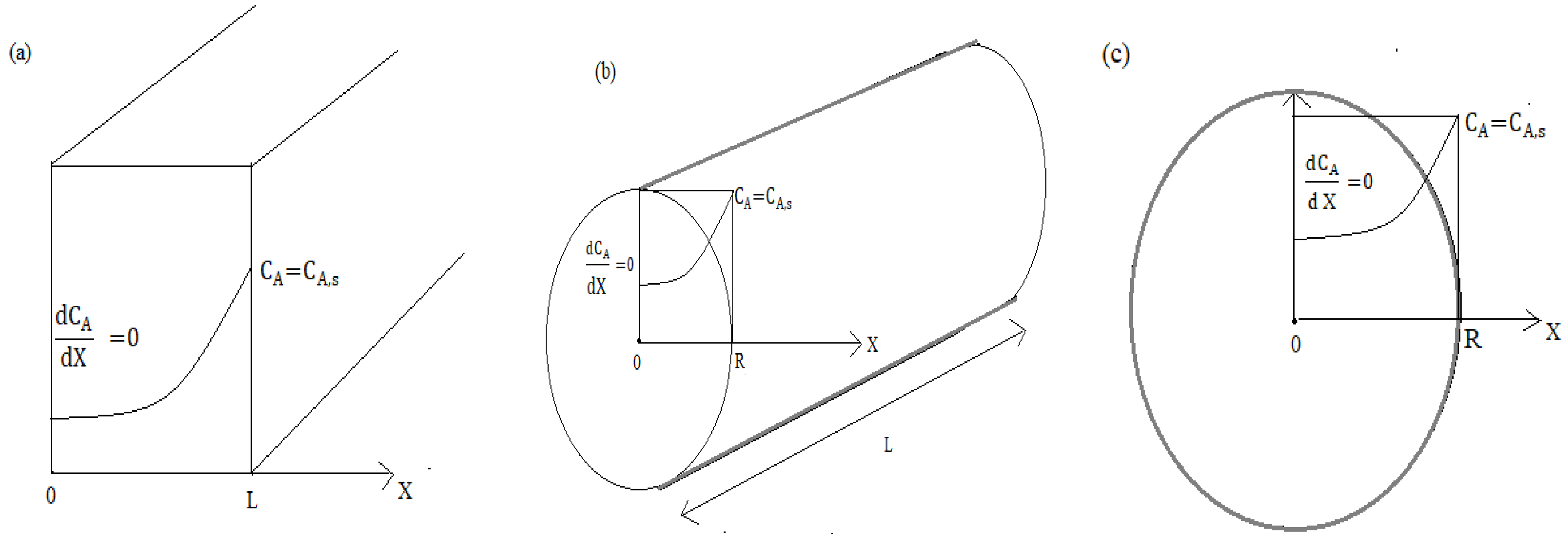
2. Mathematical Formulation of the Problem

The nonlinear mass balance equation involving heterogeneous reaction kinetics on electrochemical fixed-bed reactors of general geometries (slab, cylindrical, and spherical) can be written as follows (Appendix A):

$$\frac{d^{2}y\left(x\right)}{d x^2}+\frac{n}{x}\frac{dy\left(x\right)}{dx}={\mathsf{\Phi }}^2 y\left(x\right)e^{\left(\frac{\gamma \beta \left(1-y\left(x\right)\right)}{1+\beta \left(1-y\left(x\right)\right)}\right)}$$

(1)

The dimensionless boundary conditions are

$$\mathrm{At} x=1, y=1,$$

(2)

$$\mathrm{At} x=0, \frac{dy}{dx}=0,$$

(3)

where $y$ is the dimensionless concentration of reactant, $x$ is the dimensionless pellet radius and $\gamma$ is the dimensionless activation energy, $\beta$ is the dimensionless heat of reaction, and $\mathsf{\Phi }$ is the Thiele modulus. The values of the geometrical shape parameter fall n within the range 0 to 2 for all simply connected regions of the pellet. The limits of these regions are: the infinite slab (n = 0), cylinder (n = 1), and the sphere (n = 2).

The effectiveness factor is

$$\eta =\frac{\left(n+1\right)}{{\mathsf{\Phi }}^2}{\left(\frac{dy}{dx}\right)}_{x=1},$$

(4)

3. Approximate Analytical Expression of the Concentration and Effectiveness Factor Using Akbari-Ganji’s Method

Solving nonlinear differential equations analytically is more complicated than solving linear differential equations. Recently, many asymptotic methods for solving nonlinear differential equations have been developed, such as the homotopy perturbation method [28,29,30], Adomian decomposition method [31,32,33], Variational iteration method [34,35,36], Taylor series method [37,38], Akbari-Ganji method [39,40,41,42,43,44], and Rajendran–Joy method [45]. The AGM may be considered a powerful algebraic (semi-analytic) approach for solving such problems. The approximate analytical expression of a reactant concentration for all dimensionless parameters is obtained using this method (Appendix B) as follows:

$$y\left(x\right)=\frac{\cosh \left(mx\right)}{\cosh m}$$

(5)

where m is obtained by solving the equation

$$m^2+\left(\frac{n}{0.5}\right)m\tanh \left(0.5m\right)-{\mathsf{\Phi }}^2{e}^{\left(\frac{\gamma \beta \left(1-\cosh \left(0.5 m\right)\sec \mathrm{h}m\right)}{1+\beta \left(1-\cosh \left(0.5 m\right)\sec \mathrm{h}m\right)}\right)}=0$$

(6)

Equation (5) is the new analytical expression of a reactant concentration for all values of dimensionless parameters $\gamma$, $\beta$ and $\mathsf{\Phi }$. The Ying Buzu algorithm [46,47] can be used to find the unknown parameter m. The numerical value of $m$ for the given values of $\gamma , n, \beta$, and $\mathsf{\Phi }$ can be obtained by solving Equation (6) by any mathematical software. Additionally, when m is small, Equation (6) becomes (Appendix C):

$$m\simeq \sqrt{\frac{2{\mathsf{\Phi }}^2}{2\left(1+\mathrm{n}\right)-{\mathsf{\Phi }}^2\gamma \beta }}$$

(7)

and for large values of m, we have

$$m\simeq \sqrt{n^2+{\mathsf{\Phi }}^2{e}^{\left(\frac{\gamma \beta }{1+\beta }\right)}}-n$$

(8)

Substituting the value of $m$ in Equation (5) gives the closed-form of approximate analytical expression of a reactant concentration, $y\left(x\right),$ for all dimensionless parameters.

The regular false method and the secant algorithm were also used to determine this parameter. The Ying Buzu algorithm method offers an extremely fast convergent result. The effectiveness factor response can be obtained as follows:

$$\eta =\frac{\left(n+1\right)}{{\mathsf{\Phi }}^2}{\left(\frac{dy}{dx}\right)}_{x=1}=\frac{\left(n+1\right)}{{\mathsf{\Phi }}^2}m \tan \mathrm{h}(m)$$

(9)

4. Numerical Simulation

The nonlinear diffusion Equation (1) for the boundary conditions (Equations (2) and (3)) is also solved numerically. We have used the function pdex1 in MATLAB software to numerically solve the initial-boundary value problems for the nonlinear differential equations (Appendix D).

The simulation results are compared with our approximate analytical results in

Table 1. Comparison of dimensionless concentration of species $y\left(x\right)$ for spherical catalyst pellets with simulation results for various values of parameter $\mathsf{\Phi }$ when $\beta =0.01 \mathrm{and} \gamma =1$.

$\mathit{x}$	$\mathbf{\Phi }=0.1, \mathit{m}=0.057741$			$\mathbf{\Phi }=5,\mathbf{m}=3.48049$			$\mathbf{\Phi }=10, \mathit{m}=8.24677$
	Num	Approximate Analytical Equation (5)	Error% Equation (5)	Num	Approximate Analytical Equation (5)	Error% Equation (5)	Num	Approximate Analytical Equation (5)	Error% Equation (5)
0	0.9983	0.9983	0.0000	0.0663	0.0625	5.7315	0.0007	0.0007	0.0000
0.2	0.9984	0.9984	0.0000	0.0783	0.0774	1.1494	0.0016	0.0016	0.0000
0.4	0.9986	0.9986	0.0000	0.1222	0.1290	5.2713	0.0062	0.0062	0.0000
0.6	0.9989	0.9989	0.0000	0.2282	0.2246	1.5776	0.0315	0.0302	4.1269
0.8	0.9994	0.9994	0.0000	0.4727	0.4795	1.4385	0.1802	0.1739	3.4961
1	1.0000	1.0000	0.0000	1.0000	1.0000	0.0000	1.0000	1.0000	0.0000
	Average error (%)		0.0000	Average error (%)		2.5280	Average error (%)		1.2705

Num represents numerical results.

,

Table 2. Comparison of dimensionless concentration of species $y\left(x\right)$ for spherical catalyst pellets with simulation results for various values of parameter $\mathsf{\Phi }$ when $\mathsf{\beta }=100\mathrm{and} \gamma =1.$

$\mathit{x}$	$\mathbf{\Phi }=0.1, \mathit{m}=0.061428$			$\mathbf{\Phi }=5, \mathit{m}=6.46641$			$\mathbf{\Phi }=10,\mathit{m}=14.5272$
	Num	Approximate Analytical Equation (5)	Error% Equation (5)	Num	Approximate Analytical Equation (5)	Error% Equation (5)	Num	Approximate Analytical Equation (5)	Error% Equation (5)
0	0.9981	0.9981	0.0000	0.0045	0.0040	11.111	0.0000	0.0000	0.0000
0.2	0.9982	0.9982	0.0000	0.0069	0.0068	1.4493	0.0000	0.0000	0.0000
0.4	0.9985	0.9984	0.0100	0.0187	0.0189	1.0695	0.0001	0.0001	0.0000
0.6	0.9988	0.9988	0.0000	0.0656	0.0649	1.0671	0.0026	0.0024	7.6923
0.8	0.9994	0.9993	0.0100	0.2581	0.2548	1.2786	0.0532	0.0531	0.1880
1	1.0000	1.0000	0.0000	1.0000	1.0000	0.0000	1.0000	1.0000	0.0000
	Average error (%)		0.0033	Average error (%)		2.6626	Average error (%)		1.3134

,

Table 3. Comparison of dimensionless concentration of species $y\left(x\right)$ for spherical catalyst pellets with simulation results for various values of parameter $\mathsf{\Phi }$ when $\gamma =0.01\mathrm{and}\beta =0.01.$

$\mathit{x}$	$\mathbf{\Phi }=0.1, \mathit{m}=0.057740$			$\mathbf{\Phi }=5,\mathit{m}=3.462948$			$\mathbf{\Phi }=10, \mathit{m}=8.199400$
	Num	Approximate Analytical Equation (5)	Error% Equation (5)	Num	Approximate Analytical Equation (5)	Error% Equation (5)	Num	Approximate Analytical Equation (5)	Error% Equation (5)
0	0.9983	0.9983	0.0000	0.0673	0.0651	3.2689	0.0000	0.0000	0.0000
0.2	0.9984	0.9984	0.0000	0.0794	0.0802	1.0075	0.0017	0.0017	0.0000
0.4	0.9986	0.9986	0.0000	0.1235	0.1228	0.5668	0.0064	0.0064	0.0000
0.6	0.9989	0.9989	0.0000	0.2296	0.2264	1.3937	0.0320	0.0335	4.6875
0.8	0.9994	0.9994	0.0000	0.4738	0.4649	1.8784	0.1813	0.1908	5.2399
1	1.0000	1.0000	0.0000	1.0000	1.0000	0.0000	1.0000	1.0000	0.0000
	Average error (%)		0.0000	Average error (%)		1.3525	Average error (%)		1.6546

and

Table 4. Comparison of dimensionless concentration of species $y\left(x\right)$ for spherical catalyst pellets with simulation results for various values of parameter $\mathsf{\Phi }$ when $\gamma =100\mathrm{and}\beta =0.01$.

$\mathit{x}$	$\mathbf{\Phi }=0.1, \mathit{m}=0.057776$			$\mathbf{\Phi }=5, \mathit{m}=6.28141$			$\mathbf{\Phi }=10, \mathit{m}=14.5216$
	Num.	Approximate Analytical Equation (5)	Error% Equation (5)	Num	Approximate Analytical Equation (5)	Error% Equation (5)	Num	Approximate Analytical Equation (5)	Error% Equation (5)
0	0.9983	0.9983	0.0000	0.0071	0.0068	4.2253	0.0000	0.0000	0.0000
0.2	0.9984	0.9984	0.0000	0.0108	0.0101	6.4615	0.0000	0.0000	0.0000
0.4	0.9986	0.9986	0.0000	0.0289	0.0289	0.0000	0.0002	0.0002	0.0000
0.6	0.9989	0.9989	0.0000	0.0981	0.0956	2.5484	0.0038	0.0033	13.158
0.8	0.9994	0.9994	0.0000	0.3460	0.3401	1.7052	0.0780	0.0713	8.5874
1	1.0000	1.0000	0.0000	1.0000	1.0000	0.0000	1.0000	1.0000	0.0000
	Average error (%)		0.0000	Average error (%)		2.4906	Average error (%)		3.6242

for spherical catalyst pellets. The maximum average error percentage between numerical and our approximate analytical results is 3.6% for all values of the activation energy, heat of reaction, and Thiele modulus.

5. Discussion

Equation (5) is the new closed and simple new approximate analytical expressions’ concentration of reactant. The concentration depends on the parameters $\gamma$ (dimensionless activation energy), $\beta$ (dimensionless heat of reaction), and $\mathsf{\Phi }$ (Thiele modulus).

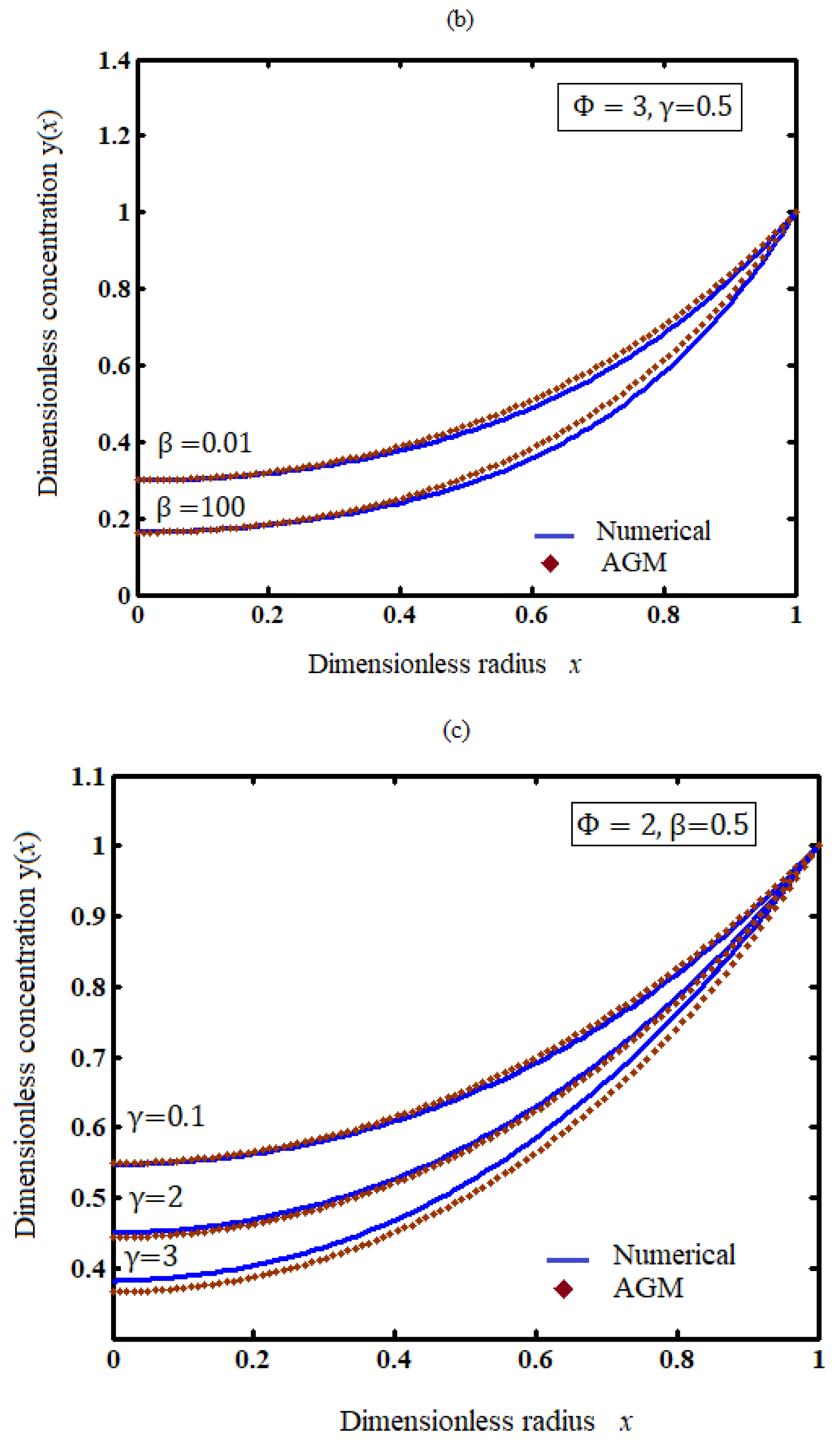
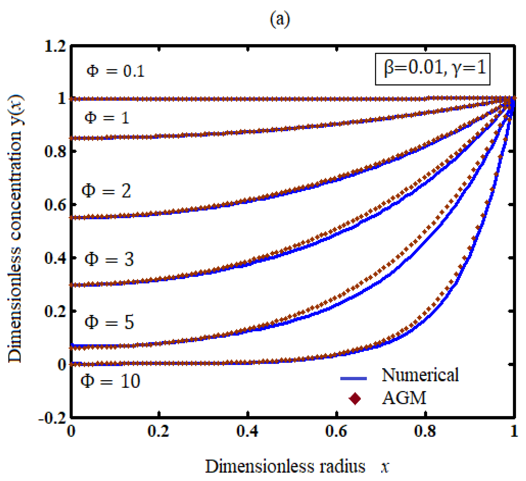
5.1. Influence of the Parameters (Thiele Modulus, Heat of the Reaction, and Activation Energy) on the Concentration Profile

The Thiele modulus is the ratio of reaction to diffusion rates. Figure 1a–c represent the concentration of species for various value parameters. Figure 1a illustrates the concentration profile for various values of the Thiele modulus. When $\mathsf{\Phi }$ is low, the diffusional resistance is inadequate to limit the reaction rate. Therefore, uniform concentration C_A/C_AS can be maintained. However, when $\mathsf{\Phi }$ is large, a significant diffusional resistance prevents a constant concentration profile of A within the catalyst particle and thus lowers the observed rate. From the figure, it is observed that the concentration increases when the Thiele modulus decreases. Additionally, the concentration is uniform when $\mathsf{\Phi }\ll 0.1$. From Figure 1b,c, it is inferred that concentration decreases when the heat of the reaction ($\beta )$ and activation energy ($E$) decreases.

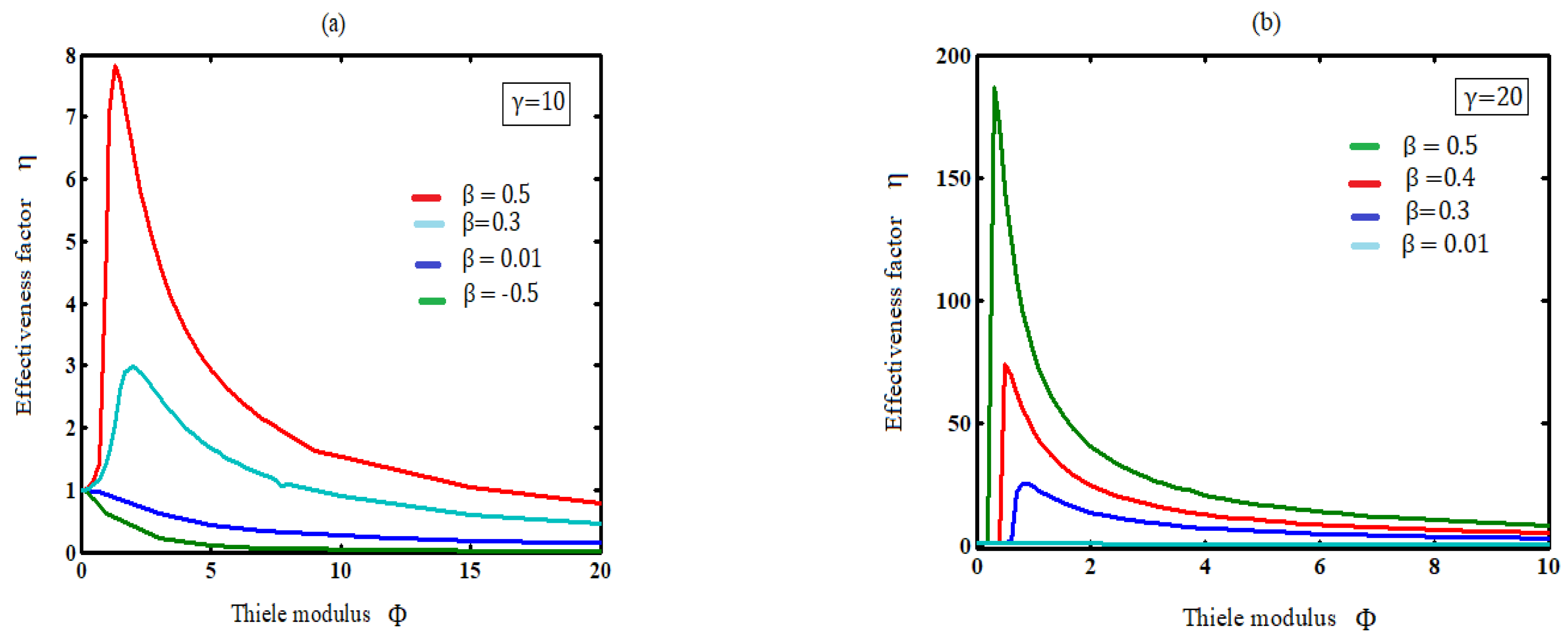
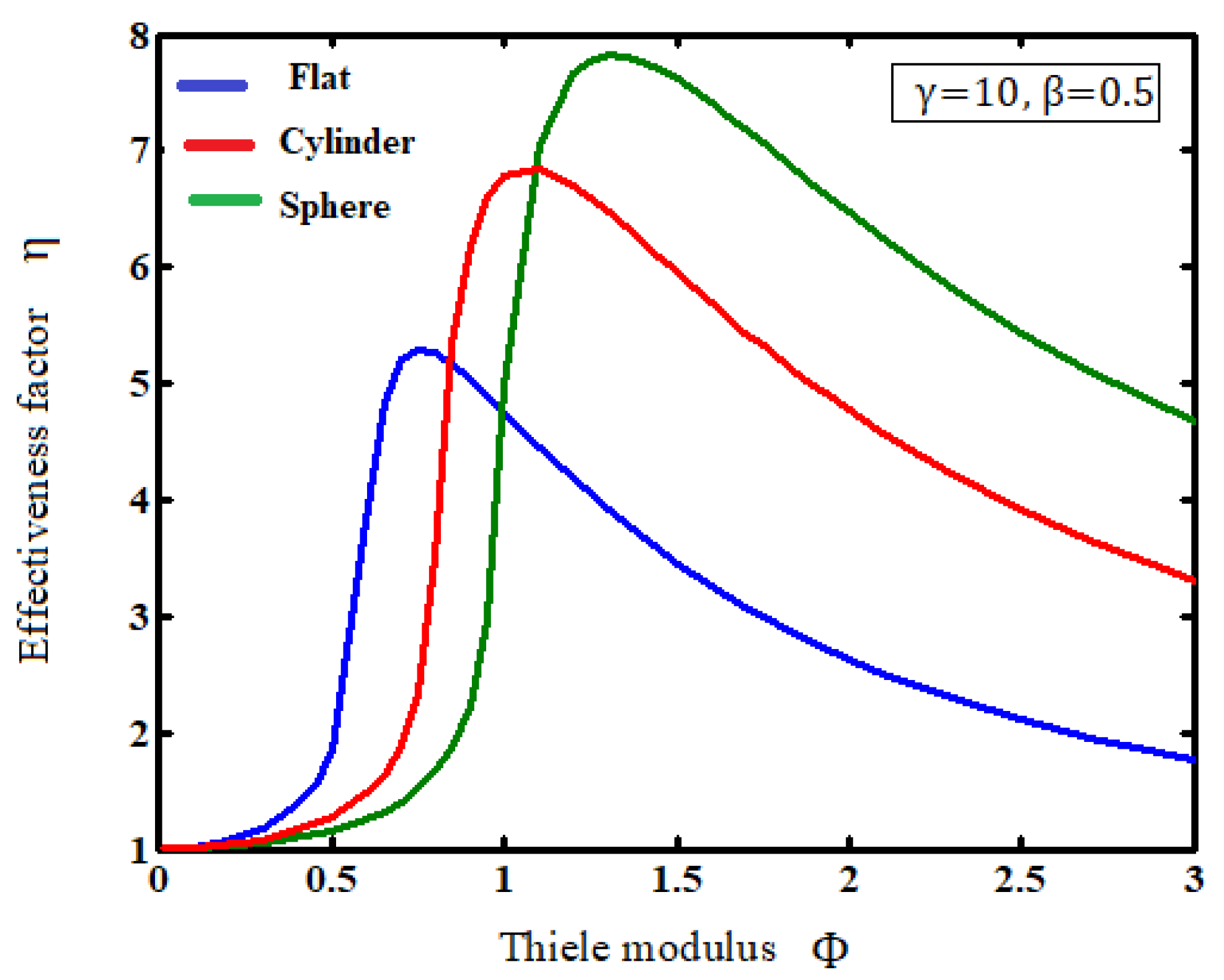
5.2. Influence of the Parameters (Thiele Modulus, Heat of the Reaction, and Activation Energy) on the Effectiveness Factor

The overall reaction rate in a catalytic pellet is often expressed by the effectiveness factor η, which measures the total reaction rate as a scalar multiple of a homogeneous reaction rate at the surface concentration.

Equation (9) represents the new approximate analytical expression of the effectiveness factor for all values of parameters. It is observed that the value of the effectiveness factor $\eta$ increases as the Thiele modulus $\mathsf{\Phi }$ increases initially, reaches the maximum value, and then decreases. The peak value of the effectiveness factor increases when the heat of the reactant $\left(\beta \right)$ or activation energy $\left(\gamma \right)$ increases. The heat of the reaction value is negative for an exothermic reaction. In this case, the effectiveness factor is less than one (see Figure 2a).

Figure 3 shows the effectiveness factor versus Thiele modulus for flat, cylindrical, and spherical catalyst pellets. It is observed that the peak value of the effectiveness factor for spherical geometrics is higher than for cylindrical and slab geometries. Furthermore, it is concluded that for all geometries, the effectiveness increases when the Thiele modulus increases to attain the maximum value before it decreases.

5.3. A limiting Case: The Dimensionless Heat of Reaction Is Zero $\left(\beta =0\right)$

When $\beta =0$, Equation (1) becomes

$$\frac{d^{2}y\left(x\right)}{d x^2}+\frac{n}{x}\frac{dy\left(x\right)}{dx}={\mathsf{\Phi }}^2 y\left(x\right)$$

(10)

In this case, we can obtain the well-known exact analytical expression of concentration and effectiveness factors when n = 0, 1, 2. In

Table 5. The concentration and effectiveness factors when $\beta =0.$

Geometry	Exact Result		This Work (Approximate Analytical Result)
	Concentration	Effectiveness Factor	Concentration	Effectiveness Factor
Spherical $(n=2$)	$y\left(x\right)=\frac{\sin \mathrm{hh}\left(\mathsf{\Phi }x\right)}{\mathrm{xcosh}\mathsf{\Phi }}$ (11)	$\frac{1}{\mathsf{\Phi }}\left[\frac{1}{tanh\left(\varphi \right)}-\frac{1}{3\varphi }\right]$ (12)	$y\left(x\right)=\frac{\cos \mathrm{h}\left(mx\right)}{\cosh m}$ (17) where m is obtained by solving the equation $m^2+2nm\tanh \left(0.5m\right)={\mathsf{\Phi }}^2$ (18)	$\eta =\frac{\left(n+1\right)}{{\mathsf{\Phi }}^2}m\tanh m$ (19)
$\mathrm{Cylindrical}(n=1$)	$y\left(x\right)=\frac{I_{0 }\left(\mathsf{\Phi }x\right)}{I_{0 }\left(\mathsf{\Phi }\right)}$ (13)	$\frac{I_{1 }\left(2\mathsf{\Phi }\right)}{\mathsf{\Phi }{I}_{0 }\left(2\mathsf{\Phi }\right)}$ (14)
Slab$(n=0$)	$y\left(x\right)=\frac{\cos \mathrm{h}\left(\mathsf{\Phi }x\right)}{\cosh \mathsf{\Phi }}$ (15)	$\frac{\tan \mathrm{h}\mathsf{\Phi }}{\mathsf{\Phi }}$ (16)

, the exact results for the limiting cases, i.e., n = 0, 1, 2 (Equations. (11) to (16)), and approximate general analytical results (Equations. (17) to (19)) for all cases (this work) are summarized.

This limiting case result for the concentration of species $y\left(x\right)$ for cylindrical catalyst pellets is compared with our approximate analytical results in

Table 6. Comparison of dimensionless concentration of species $y\left(x\right)$ for cylindrial catalyst pellets with simulation results for various values of parameter $\mathsf{\Phi }$ when $\gamma =0 \mathrm{and} \beta =0.$

$\mathit{x}$	$\mathbf{\Phi }=0.1$			$\mathbf{\Phi }=5$			$\mathbf{\Phi }=10$
	Exact Equation (13)	This Work Equation (17)	Error%	Exact Equation (13)	This Work Equation (17)	Error%	Exact Equation (13)	This Work Equation (17)	Error%
0	0.9975	0.9975	0.0000	0.0367	0.0351	4.3697	0.0003	0.0003	0.0000
0.2	0.9976	0.9976	0.0000	0.0465	0.0469	0.8602	0.0008	0.0008	0.0000
0.4	0.9979	0.9979	0.0000	0.0837	0.0821	1.9116	0.0040	0.0045	12.500
0.6	0.9984	0.9984	0.0000	0.1792	0.1753	2.1763	0.0239	0.0236	1.2552
0.8	0.9991	0.9991	0.0000	0.4149	0.4174	0.7231	0.1518	0.1607	5.8629
1	1.0000	1.0000	0.0000	1.0000	1.0000	0.0000	1.0000	1.0000	0.0000
	Average error (%)		0.0000	Average error (%)		1.6735	Average error (%)		3.2697

, where satisfactory agreement is noted.

Here we have presented an analysis to compute the effectiveness factor in a reaction/diffusion system of general geometry. The value for the effectiveness factor is also valid for a modified electrode, since the reaction flux is defined by the concentration gradient at x = 1. Therefore, the analysis for a polymer-modified electrode and a packed bed reactor are equivalent. Consequently, the theory applies to both electrochemical and catalytic problems, hence the concept applies equally to electrochemical and catalytic problems. The concept of effectiveness factor is beneficial for polymer-modified electrodes since it presents the degree of utilization of the layer in catalysis. The electrochemical polymer-modified electrode problem is equivalent to packed bed catalysis.

6. Conclusions

The mass transfer behavior in fixed electrochemical reactors was discussed. The nonlinear differential equation for coupled heat and mass transfer in a slab, cylindrical, and spherical non-isothermal kinetics was solved analytically using the efficient Akbari-Ganji method. The approximate analytical expressions for the reactant concentration and effectiveness factor were obtained for all values of parameters. The numerical simulation results provided by Matlab, and theoretical predictions, were found to be in satisfactory agreement. The derived approximate analytical results were employed to analyze the effect of the behavior of porous catalyst particles subject to both internal mass concentration gradients and temperature gradients in endothermic or exothermic reactions. The theoretical model in this study and the derived approximate analytical solution can be extended to study the electrosynthesis of chemicals and drugs, redox flow batteries, fuel cells, water disinfection, and electrodialysis.

References

1. Walsh, F. A First Course in Electrochemical; The Electrochemical Consultancy: Hants, UK, 1993. [Google Scholar]
2. Sedahmed, G.H.; Shemilt, L.W. Forced convection mass transfer at rough surfacesin annuli. Lett. Heat Mass Transf. 1976, 3, 499–511. [Google Scholar] [CrossRef]
3. Bird, R.; Stewart, W.; Lightfoot, E. Transport Phenomena, 2nd ed.; John Wiley and Sons: New York, NY, USA, 2002. [Google Scholar]
4. Treybal, R.E. Mass Transfer Operations; McGraw Hill: New York, NY, USA, 1980; p. 466. [Google Scholar]
5. Zaki, M.; Nirdosh, I.; Sedahmed, G.H. Effect of surface roughness induced bywoven metallic screens wrapped on the inner surface of an annulus on the rate of turbulent flow mass transfer. Ind. Eng. Chem. Res. 1996, 35, 4354–4359. [Google Scholar] [CrossRef]
6. El-Sherbiny, M.F.; Zatout, A.A.; Hussien, M.; Sedahmed, G.H. Mass transfer at the gas evolving inner electrode of a concentric cylinder reactor. J. Appl. Electrochem. 1991, 21, 537–542. [Google Scholar] [CrossRef]
7. Fahidy, T.Z. Electrolysis in an annular flow cell with gas generation. J. Appl. Electrochem. 1979, 9, 101–108. [Google Scholar] [CrossRef]
8. Sedahmed, G.H.; Hosny, A.Y.; Fadally, O.A.; El-Mekkawy, I.M. Mass transfer at rough gas-sparged electrodes. J. Appl. Electrochem. 1994, 24, 139–144. [Google Scholar] [CrossRef]
9. de Sa, M.S.; Shemilt, L.W.; Soegiarto, I.V. Mass transfer in the entrance region for axial and swirling annular flow. Can. J. Chem. Eng. 1991, 69, 294–299. [Google Scholar] [CrossRef]
10. Legentilhomme, P.; Legrand, J. Overall mass transfer in swirling decaying flow in an annular electrochemical cells. J. Appl. Electrochem. 1990, 20, 216–222. [Google Scholar] [CrossRef]
11. Zaki, M.M.; Nirdosh, I.; Sedahmed, G.H. Mass transfer behavior of annular ducts under developing flow with superimposed pulsating flow. Chem. Eng. Technol. 2011, 34, 475–481. [Google Scholar] [CrossRef]
12. Storck, A.; Coeuret, F. Mass transfer between a flowing liquid and a wall or animmersed surface in fixed and fluidized beds. Chem. Eng. J. 1980, 20, 149–154. [Google Scholar] [CrossRef]
13. Hutin, D.; Storck, A.; Coeuret, F. Local study of wall to liquid mass transfer influidized and packed beds. II. Mass transfer in packed beds. J. Appl. Electrochem. 1979, 9, 361–367. [Google Scholar] [CrossRef]
14. Ramana Rao, M.V.; Rao, C.V. Mass transfer in square channels. Part II–ionic mass transfer in packed beds. Ind. J. Technol. 1970, 8, 44–47. [Google Scholar]
15. Paterson, W.R.; Cresswell, D.L. A simple method for the calculation of effectiveness factors. Chem. Eng. Sci. 1971, 26, 605–616. [Google Scholar] [CrossRef]
16. Tavera, E.M. Analytical expression for the non-isothermal effectiveness factor: The nth-order reaction in a slab geometry. Chem. Eng. Sci. 2005, 60, 907–916. [Google Scholar] [CrossRef]
17. Thiele, E.W. Relation between catalytic activity and size of particle. Ind. Eng. Chem. 1936, 31, 916–920. [Google Scholar] [CrossRef]
18. Weisz, P.; Hicks, J. The behaviour of porous catalyst particles in view of internal mass and heat diffusion effects. Chem. Eng. 1962, 17, 265–275. [Google Scholar] [CrossRef]
19. Ishida, M.; Wen, C.; Shirai, T. Comparison of zone-reaction model and unreacted-core shrinking model in solid-gas reactions—II non-isothermal analysis. Chem. Eng. Sci. 1971, 26, 1043–1048. [Google Scholar] [CrossRef]
20. Kimura, S.; Tone, S.; Otake, T. Reaction order in the grain model with grain size distribution. J. Chem. Eng. Jpn. 1981, 14, 491–493. [Google Scholar] [CrossRef] [Green Version]
21. Wang, S.C.; Wen, C.Y. Experimental evaluation of nonisotheral solid-gas reaction model. AIChE J. 1972, 18, 1231–1238. [Google Scholar] [CrossRef]
22. Weisz, P.B.; Goodwin, R.D. Combustion of carbonaceous deposits within porous catalyst particles I. Diffusion-controlled kinetics. J. Catal. 1963, 2, 397–404. [Google Scholar] [CrossRef]
23. Cannon, K.J.; Denbigh, K.G. Studies on gas-solid reactions—I: The oxidation rate of zinc sulphide. Chem. Eng. Sci. 1957, 6, 145–154. [Google Scholar] [CrossRef]
24. Costa, E.C.; Smith, J.M. Kinetics of noncatalytic, nonisothermal, gas-solid reactions: Hydrofluorination of uranium dioxide. AIChE J. 1971, 17, 947–957. [Google Scholar] [CrossRef]
25. Shettigar, U.R.; Hughues, R. Prediction of transient temperature distribution in gas—Solid reactions. Chem. Eng. J. 1972, 3, 93–99. [Google Scholar] [CrossRef]
26. Lucia, A.; Gattupalli, R.R. A barrier-terrain methodology for global optimization. Ind. Eng. Chem. Res. 2008, 47, 2666–2680. [Google Scholar] [CrossRef]
27. Renugadevi, M.; Sevukaperumal, S.; Rajendran, L. The Approximate analytical solution of non-linear equation for simultaneous internal mass and heat diffusion effects. Nat. Sci. 2016, 8, 284–294. [Google Scholar] [CrossRef] [Green Version]
28. Nadeem, M.; He, J.H. The homotopy perturbation method for fractional differential equations: Part 2, two-scale transform. Int. J. Numer. Methods Heat Fluid Flow 2022, 32, 559–567. [Google Scholar] [CrossRef]
29. He, J.H.; El-Dib, Y.O. Homotopy perturbation method with three expansions for Helmholtz-Fangzhu oscillator. Int. J. Mod. Phys. B 2021, 35, 2150244. [Google Scholar] [CrossRef]
30. Vinolyn Sylvia, S.; Joy Salomi, R.; Rajendran, L.; Lyons, M.E.G. Amperometric biosensors and coupled enzyme nonlinear reactions processes: A complete theoretical and numerical approach. Electrochim. Acta 2022, 415, 140236. [Google Scholar] [CrossRef]
31. Hasan, Y.Q.; Zhu, L.M. A note on the use of modified Adomian decomposition method for solving singular boundary value problems of higher-order ordinary differential equations. Commun. Nonlinear Sci. Numer. Simulat. 2009, 14, 3261–3265. [Google Scholar] [CrossRef]
32. Jeyabarathi, P.; Kannan, M.; Rajendran, L. Approximate analytical solutions of biofilm reactor problem in applied biotechnology. Theor. Found. Chem. Eng. 2021, 55, 851–861. [Google Scholar] [CrossRef]
33. Jeyabarathi, P.; Rajendran, L.; Abukhaled, M.; Kannan, M. Semi-analytical expressions for the concentrations and effectiveness factor for the three general catalyst shapes. React. Kinet. Mech. Catal. 2022, 135, 1739–1754. [Google Scholar] [CrossRef]
34. He, J.H.; Wu, X.H. Variational iteration method: New development and applications. Comput. Math. Appl. 2007, 54, 881–894. [Google Scholar] [CrossRef]
35. Wazwaz, A.M. A comparison between the variational iteration method and Adomian decomposition method. J. Comput. Appl. Math. 2007, 207, 129–136. [Google Scholar] [CrossRef] [Green Version]
36. Abukhaled, M. Variational iteration method for nonlinear singular two-point boundary value problems arising in human physiology. J. Math. 2013, 1–4. [Google Scholar] [CrossRef] [Green Version]
37. Vinolyn Sylvia, S.; Joy Salomi, R.; Rajendran, L.; Abukhaled, M. Solving nonlinear reaction–diffusion problem in electrostatic interaction with reaction-generated pH change on the kinetics of immobilized enzyme systems using Taylor series method. J. Math. Chem. 2021, 59, 1332–1347. [Google Scholar] [CrossRef]
38. He, J.H. Taylor series solution for a third order boundary value problem arising in Architectural Engineering. Ain Shams Eng. J. 2022, 11, 1411–1414. [Google Scholar] [CrossRef]
39. Manimegalai, B.; Lyons, M.E.G.; Rajendran, L. A kinetic model for amperometric immobilized enzymes at planar, cylindrical and spherical electrodes: The Akbari-Ganji method. J. Electroanal. Chem. 2021, 880, 114921. [Google Scholar] [CrossRef]
40. Salomi, R.J.; Sylvia, S.V.; Rajendran, L.; Abukhaled, M. Electric potential and surface oxygen ion density for planar, spherical and cylindrical metal oxide grains. Sens. Actuators B Chem. 2020, 321, 128576. [Google Scholar] [CrossRef]
41. Saranya, K.; Mohan, V.; Rajendran, L. Steady-state concentrations of carbon dioxide absorbed into phenyl glycidyl ether solutions by residual method. J. Math. Chem. 2020, 58, 1230–1246. [Google Scholar] [CrossRef]
42. Akbari, M.R.; Akbari, S.; Kalantari, E.; Ganji, D.D. Akbari-Ganji’s method “AGM” to chemical reactor design for non-isothermal and non-adiabatic of mixed flow reactors. J. Chem. Eng. Mater. Sci. 2020, 11, 1–9. [Google Scholar] [CrossRef]
43. Mary, M.L.C.; Devi, M.C.; Meena, A.; Rajendran, L.; Abukhaled, M. Mathematical modeling of immobilized enzyme in porous planar, cylindrical, and spherical particle: A reliable semi-analytical approach. React. Kinet. Mech. Catal. 2021, 134, 641–651. [Google Scholar] [CrossRef]
44. Jeyabarathi, P.; Rajendran, L.; Lyons, M. Reaction-diffusion in a packed-bed reactors: Enzymatic isomerization with Michaelis-Menten Kinetics. J. Electroanal. Chem. 2022, 910, 116184. [Google Scholar] [CrossRef]
45. Salomi, R.J.; Rajendran, L. Cyclic voltammetric response of homogeneous catalysis of electrochemical reactions: Part 1. A theoretical and numerical approach for EE’C scheme. J. Electroanal. Chem. 2022, 918, 116429. [Google Scholar] [CrossRef]
46. Lakshmi Narayanan, K.; Shanthi, R.; Usha Rani, R.; Lyons, M.E.G.; Rajendran, L. Mathematical modelling of forced convection in a porous medium for a general geometry: Solution of thermal energy equation via Taylor’s series with Ying Buzu algorithms. Int. J. Electrochem. Sci. 2022, 17, 220623. [Google Scholar] [CrossRef]
47. Manimegalai, B.; Swaminathan, R.; Lyons, M.E.G.; Rajendran, L. Application of Taylor’s series with Ying Buzu Shu algorithm for the nonlinear problem in amperometric biosensors. Int. J. Electrochem. Sci. 2022, 17, 22074. [Google Scholar] [CrossRef]
48. Fucik, S.; Kufner, A. Nonlinear Differential Equations; Elsevier: Prague, Czech Republic, 2014; pp. 1–136. [Google Scholar]
49. Hermann, M.; Seravi, M. Nonlinear Ordinary Differential Equations; Springer: New Delhi, India, 2016. [Google Scholar]
50. Akbari, M.R.; Ganji, D.D.; Nimafar, M.; Ahmadi, A.R. Significant progress in solution of nonlinear equations at displacement of structure and heat transfer extended surface by new AGM approach. Front. Mech. Eng. 2014, 9, 390–401. [Google Scholar] [CrossRef]
Figure 1. Effect of the parameters Φ ,   β ,   and   γ on concentration of the reactant y ( x ) for spherical catalyst pellet using Equation (5). (a) Various values of Φ , (b) various values of β and (c) various values of γ .
Electrochem 03 00046 g001aElectrochem 03 00046 g001b
Figure 2. Plot of the effectiveness factor η (spherical catalyst pellets) versus the Thiele modulus Φ for various values of parameter β (a) when γ = 10 (b) when γ = 20 using Equation (9).
Electrochem 03 00046 g002
Figure 3. The effectiveness factor η versus of the Thiele modulus Φ for the flat, cylindrical, and spherical catalyst pellet.
Electrochem 03 00046 g003