Article

Robust Variable Selection Based on Relaxed Lad Lasso

1
The Graduate School, Woosuk University, Wanju-gun 55338, Korea
2
College of Economics, Hebei GEO University, Shijiazhuang 050031, China
3
School of Business Administration, Chongqing Technology and Business University, Chongqing 400067, China
4
HBIS Supply Chain Management Co., Ltd., Shijiazhuang 050001, China
5
Hebei Center for Ecological and Environmental Geology Research, Hebei GEO University, Shijiazhuang 050031, China
6
Reaserch Center of Nutural Resources Assets, Hebei GEO University, Shijiazhuang 050031, China
7
Hebei Province Mineral Resources Development and Management and the Transformation and Upgrading of Resources Industry Soft Science Resrarch Base, Shijiazhuang 050031, China
*
Authors to whom correspondence should be addressed.
Symmetry 2022, 14(10), 2161; https://doi.org/10.3390/sym14102161
Submission received: 11 September 2022 / Revised: 1 October 2022 / Accepted: 11 October 2022 / Published: 15 October 2022
(This article belongs to the Special Issue Symmetry in Functional Analysis and Engineering Mathematics)

Abstract

:
Least absolute deviation is proposed as a robust estimator to solve the problem when the error has an asymmetric heavy-tailed distribution or outliers. In order to be insensitive to the above situation and select the truly important variables from a large number of predictors in the linear regression, this paper introduces a two-stage variable selection method named relaxed lad lasso, which enables the model to obtain robust sparse solutions in the presence of outliers or heavy-tailed errors by combining least absolute deviation with relaxed lasso. Compared with lasso, this method is not only immune to the rapid growth of noise variables but also maintains a better convergence rate, which is O p n 1 / 2 . In addition, we prove that the relaxed lad lasso estimator has the property of consistency at large samples; that is, the model selects the number of important variables with a high probability of convergence to one. Through the simulation and empirical results, we further verify the outstanding performance of relaxed lad lasso in terms of prediction accuracy and the correct selection of informative variables under the heavy-tailed distribution.

1. Introduction

With the expansion of datasets, selecting factors that truly affect the response variable from enormous predictors has been a topic of interest for statisticians for many years. However, the response variable commonly contains heavy-tailed errors or outliers in practice. In such a situation, traditional variable selection techniques may fail to produce robust sparse solutions. In this paper, a new estimator for the heavy-tailed distribution data is suggested as a way to deal with this problem.
In the past two decades, Tibshirani [1] first combined ordinary least square (OLS) with L 1 penalty and proposed a new variable selection method named least absolute shrinkage and selection operator (lasso). Lasso is a convex regularization method by adding L 1 norm, which avoids the influence of the sign of OLS on the prediction results. The method can also perform simultaneously model selection and shrinkage estimation in high-dimensional data. However, lasso is sensitive in the case of heavy tails on the model distribution, which arises from the problem of heterogeneity due to the data coming from different sets [2]. So, any small changes in the data can cause the solution path of lasso to contain many irrelevant noise variables. The above instability can also occur when a single relevant covariate is randomly selected. It means that applying lasso to the same data may generate widely different results [3]. In addition, the convergence speed of lasso can be affected by the rapid growth of noise variables, and the convergence speed itself is slow. Relaxed lasso was proposed to overcome the influence of noise variables and perform variable selection at a faster and more stable speed. Meinshausen [4] defined the relaxed lasso estimator for λ 0 , and ϕ 0 , 1 as
β ^ R l a s s o = arg min β Y j = 1 p X j T β j · 1 M 2 2 + ϕ λ j = 1 p | β j | ,
where M 1 , , p , p is the number of variables with nonzero coefficients selected into the model, and 1 M is an indicator function, that is 1 M = 0 , t M 1 , t M , for all t 1 , , p . Hastie et al. [5] extended the work of Bertsimas et al. by comparing the lasso, forward stepwise and relaxed lasso methods with different signal-to-noise ratios (SNRs) scenarios. The results show that relaxed lasso has an overall outstanding performance at any SNR level. This superiority is reflected in the relaxation parameter ϕ . By appropriately modifying the parameter ϕ , relaxed lasso ensures that the resulting model is consistent with the true model, neither favoring excessive compression that would result in the exclusion of essential variables nor selecting redundant noise variables. This serves as the main reason why we add the relaxation parameter ϕ to the lad lasso. Compared to lasso, relaxed lasso greatly reduces the number of false positives while also achieving a trade-off between low computational complexity and fast convergence rates [6]. From the perspective of the closed-form solution, Mentch and Zhou [7] indicate that the relaxed lasso estimator can be expressed as a weighted average of lasso and least squares. When the weight of the lasso is increased, it provides a greater amount of regularization, hence reducing the degree of freedom of the variables in the final model to achieve sparse solutions. Bloise et al. [8] demonstrated that relaxed lasso has higher predictive power because it is able to avoid overfitting by tuning two separate parameters. He [9] concluded that relaxed lasso improves prediction accuracy since it avoids selecting unimportant variables and excessively removing informative variables. Extensive research has demonstrated that relaxed lasso has advantages in terms of variable selection, prediction accuracy, convergence speed, and computational complexity. However, relaxed lasso, like OLS cannot produce reliable solutions when the response variable contains heavy-tailed errors or outliers.
In order to solve the problem of poor fitting results of relaxed lasso to the heavy-tailed distribution or outliers, least absolute deviation (LAD) based on robust regression is introduced. It estimates coefficients by minimizing the sum of the absolute values of the prediction errors. The traditional squared loss in the objective function used by classic regularization methods is unsuitable for heavy-tailed distributions and outliers, but LAD performs admirably in these situations. Gao [10] showed that the LAD loss could provide a powerful alternative to the squared loss. In recent years, some researchers have combined robust regression with popular penalty regularization methods. The most typical method is the lad lasso of Wang et al. [11], which combines lad and adaptive lasso so that the model can perform robust variable selection. Then, the theoretical properties of lad lasso under large samples have been systematically studied by Gao and Huang [12] and Xu and Ying [13]. Arslan [14] proposed a weighted lad lasso to mitigate the effect of outliers on explanatory and response variables. In addition, lad lasso also has a wide range of practical applications. For example, Rahardiantoro and Kurnia [15] showed that lad lasso has a more minor standard error than lasso in the presence of outliers in high-dimensional data via simulation. Zhou and Liu [16] also applied the lad lasso to the double-truncated data and showed that it is more accurate to select the real model than the best subset selection procedure. Li and Wang [17] applied lad lasso to the change point problem in fields such as statistics and econometrics. Thanks to the superior performance of lad lasso, we consider proposing a new estimator that can not only perform variable selection but is also insensitive to the heavy-tailed distribution or outliers in the response variable.
In this article, we combine lad lasso and the relaxation parameter of relaxed lasso to propose relaxed lad lasso and study its asymptotic properties in the case of large samples. It integrates the advantages of relaxed lasso and lad lasso methods into the following three points. Firstly, the relaxed lad lasso estimator has the same consistency property as the lad lasso, i.e., the method selects important variables with a high probability of convergence to one. Secondly, since relaxed lasso has a closed-form solution, solving relaxed lad lasso is eventually equivalent to solving the LAD program, so we can employ a simple and efficient algorithm. Thirdly, relaxed lad lasso possesses the robustness of lad lasso to heavy-tailed errors or outliers in the response variable. In theory, we prove the n -consistency of relaxed lad lasso under some mild assumptions and illustrate its advantages in convergence speed. Although the convergence speed of the relaxed lad lasso O p n 1 / 2 is slower than that of relaxed lasso O p n 1 , our method handles outliers and heavy-tailed errors well because it is not affected by the rapid growth of noise variables. The simulation shows that relaxed lad lasso has the highest prediction accuracy and probability of the correct selection of important variables under heavy-tailed distributions compared to other methods. We also apply relaxed lad lasso to financial data and obtain the same results as the simulation regarding prediction accuracy.
However, our method has room for improvement, as LAD cannot handle the presence of outliers in the explanatory variables and is sensitive to leverage points [18]. Hence, our method suffers from the same problem. Under the framework of LAD regression, researchers have proposed many new methods to improve robustness by reducing the weight of leverage points. Giloni et al. [19] proposed a weighted least absolute deviation process (WLAD) to overcome the shortcomings of the LAD method. However, as the proportion of outliers increases, the robustness of the WLAD estimator significantly decreases [20]. To obtain a high robustness estimator and abnormal information of observations, Gao and Feng [21] proposed a penalized weighted least absolute deviation (PWLAD) regression method. Jiang et al. [22] combined the PWLAD estimator and the lasso method to detect outliers and select variables robustly. However, it is worth noting that these methods mainly address the robustness problem when there are leverage points or outliers in the explanatory variables. Still, our method is suitable in situations with heavy-tailed errors or outliers in the response variable. In the simulation, we assume that the model error follows a heavy-tailed distribution such as the t-distribution. Therefore, we do not compare relaxed lad lasso with the above methods due to the different application scenarios. More specific details can be found in Section 4.
The remainder of the paper is organized as follows: Section 2 defines the estimator of relaxed lad lasso and interprets the parameters in the model. In addition, we give the detailed procedure of the algorithm. Section 3 describes the asymptotic properties of the loss function and provides the theorems’ assumptions. Section 4 compares the performance of relaxed lad lasso with conventional lasso methods (such as classical lasso, adaptive lasso, and relaxed lasso) through simulations under different heavy-tailed distribution scenarios. Section 5 analyzes empirical data to confirm the robustness of the proposed method to heavy-tailed distributions. Section 6 summarizes the advantages of the new method as well as suggestions for further research. The proofs of the theorems are given in Appendix A, Appendix B, Appendix C, Appendix D, Appendix E.

2. Relaxed Lad Lasso

2.1. Definition

This article considers the linear model
Y = X T β + ε .
The random error term ε does not require it to obey a certain normal distribution like the traditional regression model. In this model, the condition of random error on the distribution is relaxed, and only the median is 0. X = X 1 , , X p is an n × p dimensional matrix from a normal distribution with mean 0 and variance Σ , where X i is the predictor matrix of the ith variable and Y is an n × 1 vector of response variables. β = β 1 , , β j T is the regression coefficient of the model. In addition, the regression coefficient is nonzero when j p .
Next, we define relaxed lad lasso, which combines the L 1 penalty term with the relaxation parameter ϕ , so that the new model can still maintain excellent convergence speed and variable selection ability when there are outliers in the heavy-tailed distribution and the response variable.
Definition 1.
The solution to relaxed lad lasso is
β ^ R e l a d l a s s o = arg   min β Y j = 1 p X j T β j · 1 S λ + n λ ϕ j = 1 p β j ,
where 1 S λ is an indicator function, S λ = 1 t p β ^ t λ 0 is the set of nonzero coefficients; the penalty parameter λ 0 , and ϕ 0 , 1 .
When a regression coefficient belongs to the set S λ , it is selected into the true model. If the parameters within the range of the S λ set take different values, the model will have different functions. The value of the penalty parameter λ indicates the degree of compression applied to the coefficients so that it controls the number of predictors entering the model. When either λ or ϕ takes 0, minimizing the objective function for relaxed lad lasso is equivalent to solving the LAD method, and the original intention of variable selection is lost, so the parameters always start from a value far from 0. In this paper, the optimal parameters λ , ϕ are chosen through cross-validation, and the relaxed lad lasso estimator will be consistent if the important variables are correctly selected.
We define the loss function of relaxed lad lasso as
L λ , ϕ = E Y X T β ^ σ 2 .

2.2. Algorithm

In the following, we provide a detailed algorithm for solving relaxed lad lasso as defined in (3). It is well known that the closed-form solution of relaxed lasso is a linear combination of the lasso and least squares estimator. The same form of the solution can be extended to relaxed lad lasso. It turns out that the relaxed lad lasso estimator β ^ R e l a d l a s s o is the combination of the lad lasso estimator β ^ L a d l a s s o and the LAD estimator β ^ L a d , so we can solve them separately.
Computationally, the relaxed lad lasso estimator can be written as
β ^ R e l a d l a s s o = ϕ β ^ L a d l a s s o + 1 ϕ β ^ L a d ,
where the parameter ϕ 0 , 1 . Firstly, we are interested in estimating β ^ L a d l a s s o by minimizing the convex problem
β ^ L a d l a s s o = argmin β i = 1 n Y i X i β + n λ j = 1 p β j .
A new dataset Y i , X i with i = 1 , , n + p can be considered to transform the lad lasso solution in (6) to the conventional LAD citerion. We set Y i , X i = Y , X i for 1 < i < n and Y n + k , X n + k = 0 , n λ d k for 1 k p , where d k = 0 , , 0 , 1 k th , 0 , , 0 such that the kth component is equal to 1 and the remaining components are equal to 0. It should be noted that the lad lasso estimator can be expressed as follows:
β ^ L a d l a s s o = argmin β i = 1 n + p Y i X i β .
Therefore, the computational effort of solving all lad lasso solutions in (7) is identical to that of computing any unpenalized LAD program. Then, we consider the following lad lasso solution
β ^ L a d = argmin β i = 1 n Y i X i β .
If β ^ j l a d 0 , 1 j p , then the subgradient of (8) is given by
d Y X β 1 d β j = X T sgn Y X β ^ j l a d .
So, the solution of the LAD is given by iterating
β ^ k + 1 L a d = β ^ k L a d α X T sgn Y X β ^ k L a d ,
where k is the number of iterations and α > 0 is a suitable step size.
The unpunished LAD program in (8) can be solved using the rq function in the quantreg package of R. The overview of the algorithm is described in Algorithm 1.
Algorithm 1 The algorithm for relaxed lad lasso
Input: Design matrix X R n × p , response vector Y R n , parameter ϕ 0 , 1 , iteration number k, stepsize α
Output: The relaxed lad lasso estimator β ^ R e l a d l a s s o
Initialization: Define β ^ R e l a d l a s s o = ϕ β ^ L a d l a s s o + 1 ϕ β ^ L a d
Compute
1:
Set Y i , X i with i = 1 , , n + p to be the new dataset of lad lasso
2:
Set Y i , X i = Y i , X i for 1 i n and Y n + k , X n + k = 0 , n λ d k for 1 k p , where d k = 0 , , 0 , 1 k th , 0 , , 0
3:
The objective functions of Ladlasso and LAD are Q β = argmin β i = 1 n + p Y i X i β and Q β = argmin β i = 1 n Y i X i β
4:
Set k = 0
Repeat
5:
Update β ^ k + 1 L a d β ^ k L a d α X T sgn Y X β ^ k L a d
6:
Update β ^ k + 1 L a d l a s s o β ^ k L a d l a s s o α X T sgn Y X β ^ k L a d l a s s o
7:
Update k = k + 1
Until convergence

3. The Asymptotic Properties of Relaxed Lad Lasso

Before obtaining the asymptotic properties, we must first set certain conditions. Regarding the covariance matrix Σ , we consider the settings in Fu and Knight [23] and Meinshausen [4] and put forward the first hypothesis:
Assumption 1.
For all n N , the covariance matrix cov X = Σ is diagonally dominant. According to the setting of Fu and Knight [23]:
1 n i = 1 n X i X i T Σ , as n ,
and then, it can be deduced to obtain
1 n m a x 1 i n X i T X i 0 , as n .
Obviously, the default precondition for diagonal dominance of the covariance matrix is that the covariance matrix exists. When the strong condition of diagonal dominance is satisfied, the covariance matrix is positive definite, and the hidden condition is that its inverse matrix still exists.
Assumption 2.
There exist constants c > 0 and s 0 , 1 such that the number of predictors p grows exponentially with the number of observed variables n. It can be written as
p n s e c n .
Assumption 2 sets the growth mode of p to satisfy the requirement that relaxed lad lasso still retains a better convergence speed in variable selection.
Assumption 3.
Define the range L of the penalty parameter λ. For a constant c > 0 , we have
L = λ 0 : c e p n n .
Assumption 3 sets the range of penalty parameters necessary to prove consistency.
Assumption 4.
The random error term ϵ i does not follow any distribution and has a median of 0.
In other variable selection models, such as lasso and adaptive lasso, the random error term ϵ i usually obeys the normal distribution. However, for the study of relaxed lad lasso in this paper, the distribution conditions for the random error term are relaxed, and only the median is imposed. All of the above assumptions are necessary for proving the consistency of relaxed lad lasso.
Lemma 1.
Let lim inf n n * n 1 R with R 2 . L n * λ , ϕ be an empirical loss function of L λ , ϕ , where n * is its sample size. Then, under Assumptions 1–4,
sup λ L , ϕ > 0 L λ , ϕ L n * λ , ϕ = O p n 1 / 2 log n , n .
Lemma 1 will be used to prove the key conclusion in Theorem 4.
According to Lemma 1 of Wang et al. [11], lad lasso’s oracle property is dependent on the n -consistency, that is, n a n 0 . Therefore, a n is in a sequence with o ( n 1 / 2 ) as n . The lad lasso model in this article uses a fixed λ because a n is the largest λ in the nonzero parameters; then, you can obtain λ = o ( n 1 / 2 ) .
Theorem 1.
In order to describe the loss under the lad lasso estimator when n , according to Assumptions 1–4, we have:
inf λ L λ = O p n 1 / 2 .
Theorem 1 first proves the convergence rate of lad lasso. Lad lasso uses the L 1 loss function. According to Pesme and Flammarion [24], it is shown that the L 1 loss function is non-strongly convex. Since the loss function does not have non-derivable points, we can still think that the algorithm is convex. The L 1 loss’s non-strong convexity can guarantee O n 1 / 2 convergence speed before and after iteration, and smoothness has no effect on the above conclusion, which indirectly proves that our conclusion is correct.
Theorem 2.
In order to describe the loss under the relaxed lad lasso estimator when n , according to Assumptions 1–4, we have:
inf λ , ϕ L λ , ϕ = O p n 1 / 2 .
One of the main contributions of our paper is to prove that the convergence speed of relaxed lad lasso is equivalent to that of lad lasso, even although adding the relaxation parameter ϕ does not improve the convergence speed of relaxed lad lasso. However, when the number of variables p grows exponentially with the sample n, the number of potential noise variables likewise increases significantly, but this will not slow down the convergence speed of relaxed lad lasso. Although the convergence speed of relaxed lad lasso is not ideally as fast as relaxed lasso, it still outperforms lasso due to the existence of L 1 loss and relaxation parameter ϕ , which offers good stability.
Theorem 3.
Under the condition that the design matrix is positive definite and the prediction error ε i is continuous and has a positive density at the origin, when n a n 0 , the estimator of relaxed lad lasso is n -consistency for ϵ > 0 , which is
lim n P Q β ^ Q β > ϵ = 0 .
Another major contribution of this paper is to prove that the the relaxed lad lasso estimator is consistent, where the conclusion of Lemma 1 of Wang et al. [11] in lad lasso is an essential precondition that the important variable’s penalty parameter can converge to 0 faster than n 1 / 2 . It guarantees the consistency of lad lasso, and our proof is also based on this conclusion.
Theorem 4.
Let L λ ^ , ϕ ^ be the loss of the relaxed lad lasso estimate and λ ^ , ϕ ^ chosen by K-fold cross-validation with 2 K . Under assumptions of relaxed lasso, it holds that
L λ ^ , ϕ ^ = O p n 1 / 2 log n .
We still use K-fold cross-validation when choosing the penalty parameters; that is, we select the optimal penalty parameters λ ^ and ϕ ^ by minimizing the empirical loss function of cross-validation. First, define the empirical loss function on a different observation set from R = 1 , , K as
L c v λ , ϕ = K 1 R = 1 K L R , n ˜ λ , ϕ ,
where each partition of R consists of n ˜ observations and L R , n ˜ λ , ϕ is the empirical loss of the response variable.

4. Simulation

4.1. Setup

In this section, we present the results of extensive simulations that are conducted to assess how relaxed lad lasso performs in the presence of heavy-tailed errors. For comparison, the performances of the proposed relaxed lad lasso, lasso, lad lasso, and relaxed lasso are evaluated along with some metrics through the results of the mean and median of the mean absolute prediction error (MAPE), the average number of nonzero estimated coefficients (number of nonzeros), and the average number of correctly (mistakenly) estimated zeros. The above metrics are selected the same as Wang et al. [11] and Hastie et al. [5]. The procedure for setting parameters can be summarized as follows:
  • We consider the following regression model Y = X T β + σ ε in this simulation. The predictor matrix X is generated from a p-dimension multivariate normal distribution N 0 , Σ where the covariance matrix Σ i j = ρ i j with ρ = 0.5 . ε is derived from several heavy-tailed distributions. The density function of the t-distribution shows a heavy tail compared to the standard normal distribution. Therefore, we set ε to follow t-distribution with 5 degrees of freedom df( t 5 ) and the standard t-distribution with 3 degrees of freedom df( t 3 ).
  • We set the fixed dimension p = 8 and vary n = 50 , 100 , 200 to compare the performances of four methods under different sample sizes.
  • The true regression cofficient β = ( 0.5 , 1 , 1.5 , 2 , 0 , 0 , 0 , 0 ) is an eight-dimension vector where its first four elements are important variables taking nonzero coefficients and otherwise set as 0.
  • The value of σ is adjusted to achieve different theoretical SNR values. We discuss σ = 0.5 and σ = 1 in order to test the effects of strong and weak SNR values on the results.
  • The parameter λ is selected by the five-fold cross-validation, and the mean absolute error is applied for the loss of cross-validation. In addition, 100 simulation iterations are completed for each situation to test the performance of relaxed lad lasso.

4.2. Evaluation Metrics

In order to select the optimal parameters by cross-validation, we divide the data into a training set and a test set. Assume that x t e s t represents a row from the test set’s predictor matrix X and that β ^ and y ^ t e s t are the estimated coefficients and the fitting results of x t e s t on the test set. The evaluation metrics we use are shown as follows.
The mean absolute prediction error (MAPE):
MAPE = E Y t e s t y ^ t e s t = E Y t e s t x t e s t T β ^ .
The number of nonzero estimated coefficients (number of nonzeros):
Number of nonzeros = β ^ 0 = i = 1 p 1 β ^ i 0 .
The number of correctly (mistakenly) estimated zeros (number of zeros):
Correct = i = 1 p 1 β ^ i = 0 , β i = 0 .
Incorrect = i = 1 p 1 β ^ i = 0 , β i 0 .

4.3. Summary of Results

As can be seen, the results of the simulation are summarized in Table 1 and Table 2. From the view of the number of selected nonzero and zero variables, all of the methods are shown to be comparable; however, the mean and median results of prediction accuracy are rather different. When the SNR is low (i.e., σ = 0.5 ), relaxed lad lasso outperforms lasso, lad lasso, and relaxed lasso with the lowest mean and median of MAPE. Additionally, relaxed lad lasso almost correctly identifies the number of noise variables in the sense that the variable selection results come close to the number of zero coefficients in the true model. In particular, since the real regression model has four variables that are nonzero, relaxed lad lasso correctly selects the number of important variables that is closest to the actual nonzero variables. When the SNR is high (i.e., σ = 1.0 ), all methods perform slightly worse than the low SNR situation; nevertheless, relaxed lad lasso remains a competitive method and consistently performs well on these evaluation metrics.
It is worth noting that as the number of observations n increases, the difference between the results of relaxed lad lasso and the worst methods with the same SNR value becomes smaller. For σ = 0.5 with t 5 error, the numerical difference between the relaxed lad lasso and the lad lasso’s mean MAPE is 0.043 in a small number of observations, i.e., n = 50 . When n increases to 200, the difference between them drops to 0.023. Therefore, relaxed lad lasso stands out when n is small, but as n increases, the advantage of relaxed lad lasso starts to decrease because, in that case, the data asymptotically follow a normal distribution that breaks the condition of heavy-tailed distributions we required. Therefore, we can conclude that in a normal distribution, the performance of relaxed lad lasso is comparable to the traditional robust regression and ordinary lasso method. However, when data have a heavy-tail distribution, relaxed lad lasso has an overall superior performance in terms of prediction accuracy and correct selection of the number of important information variables.

5. Application to Real Data
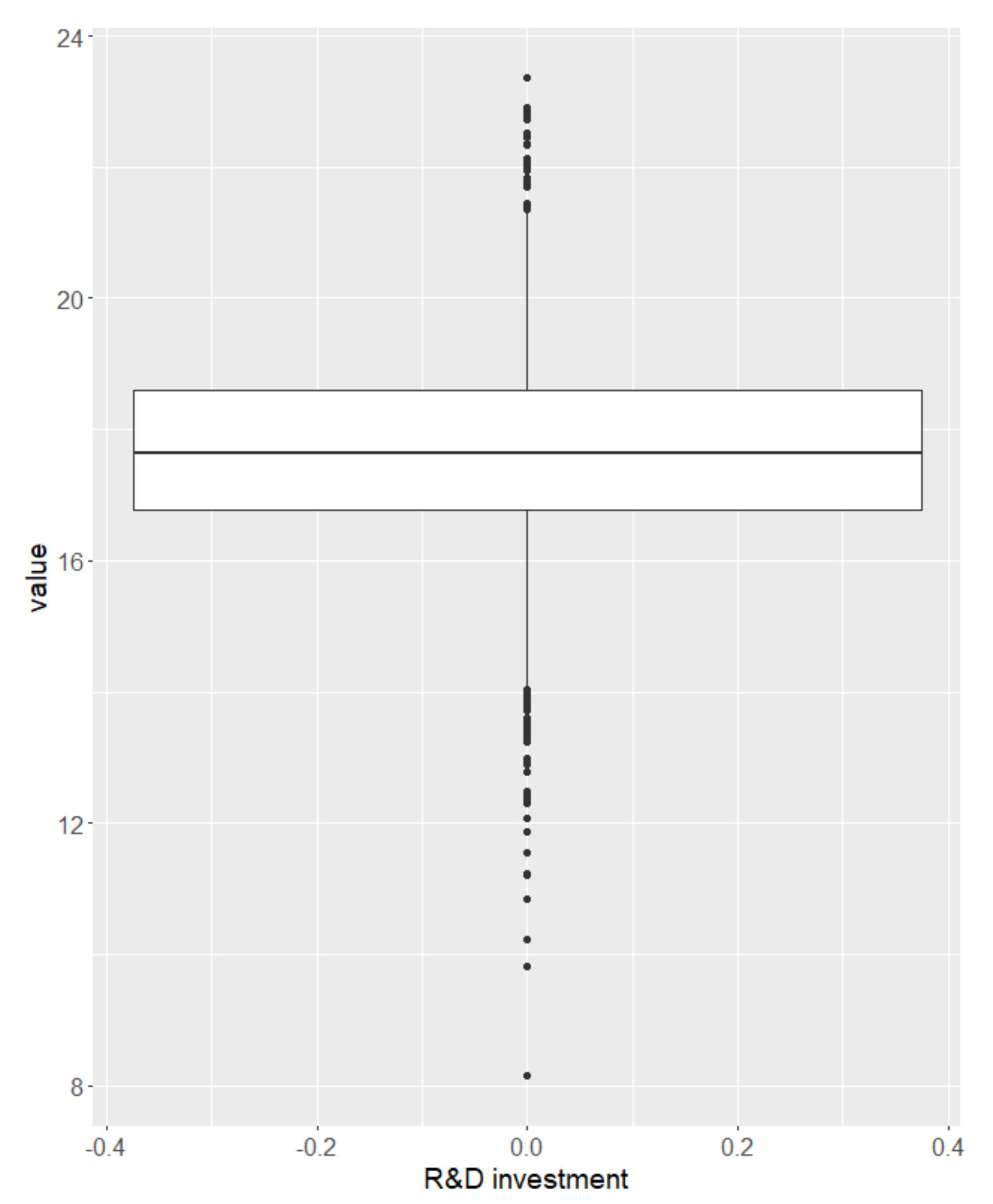
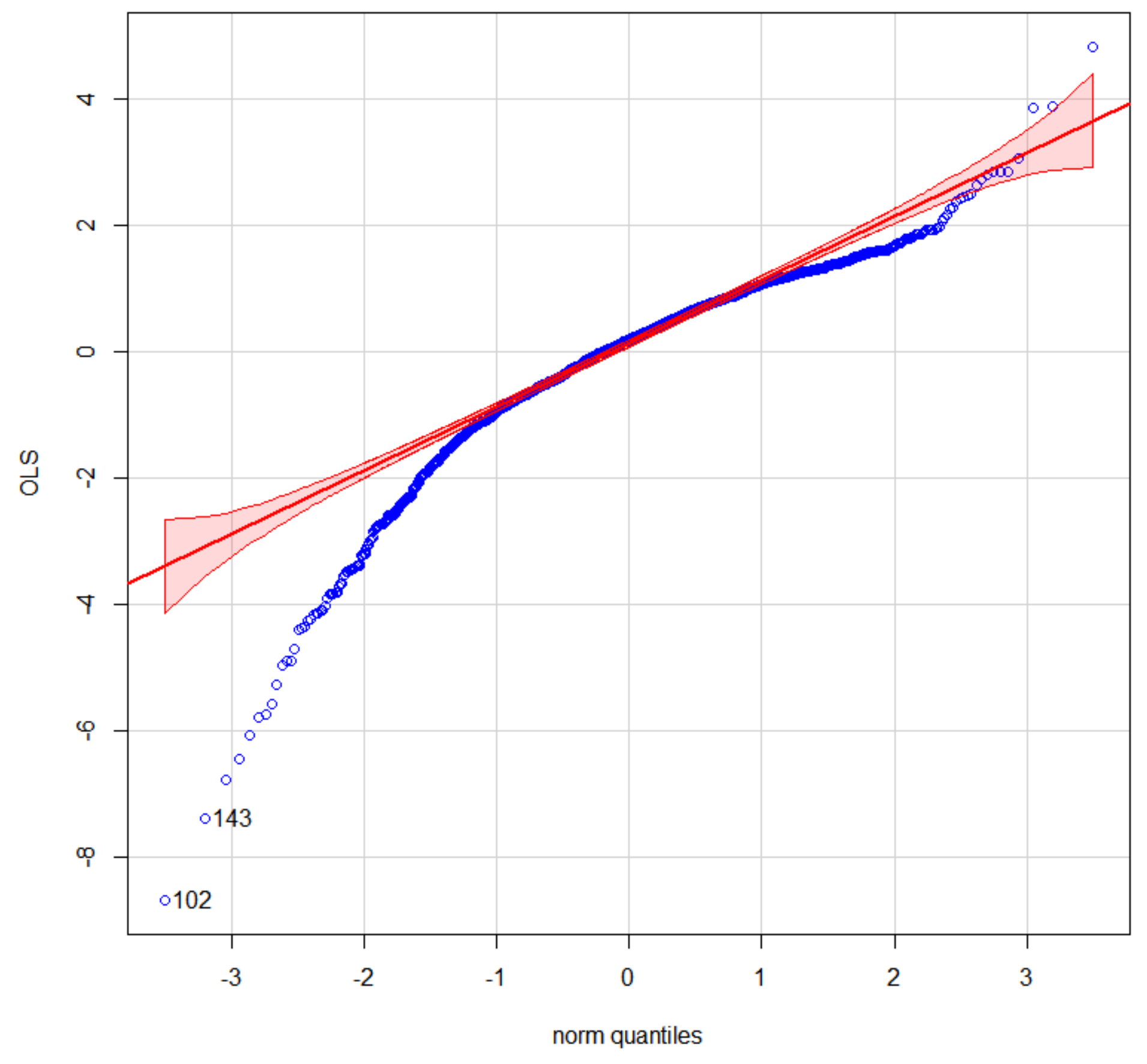
5.1. Dataset

The Research and Development (R&D) investment is critical for a company’s operations in the current competitive environment, regardless of industry. The problem of identifying the primary factors affecting the R&D investment has been extensively researched to maintain competitiveness and improve innovation. The real data for this study came from the CSMAR database, which is considered one of the most professional and extensively used research databases available. The data have 2137 records, each of which corresponds to the financial data of a single publicly traded firm in 2021. We split the data into a training set and a test set with with a ratio of 7:3 so that the training set can be used to fit the model and the MAPE is measured on the test set. The R&D investment of a corporation is the response variable, and there are 86 predictor variables, such as management costs, operating costs, net profit, and other financial indicators that may impact a company’s R&D expenditure. Table 3 provides a full overview of these factors. Due to the large variance in the R&D investment between industries, the response variables may have heavy-tailed errors or outliers. Therefore, we check to find that the residuals differentiated by an OLS fit have a kurtosis of 144.38, which is significantly greater than the normal distribution’s value. Furthermore, we show the box plot of R&D investment and the QQ-plot of the OLS fit in Figure 1 and Figure 2. The block dots in Figure 1 and the blue dots outside the 95% confidence interval in Figure 2 indicate that the response variable contains a large number of outliers. Note that we take the logarithm of the response value. Consequently, the dependability of conventional OLS-based estimators and model selection methods (e.g., lasso, relaxed lasso) is substantially compromised. To confirm the previously stated conclusion in Section 5, we continue to calculate the MAPE to compare the performances of the four methods that appear in the simulation.

5.2. Analysis Results

In Table 4, relaxed lad lasso outperforms all competitors in terms of prediction accuracy, with the smallest MAPE of 0.184, as has been demonstrated in the simulation. Lad lasso and relaxed lasso have MAPEs of 0.201 and 0.191, respectively. Lasso is the worst method. Specifically, the MAPE of lasso is 0.203, which is slightly larger than that of lad lasso. The relevant variables selected by the best resulting model are listed in Table 5. We find that Net Accounts Receivable, Funds Paid to and for Staff, Other Income, Gains and Losses from Asset Disposition, Interest Income, and Basic Earnings Per Share are the most important factors influencing the R&D spending. Therefore, we can conclude that relaxed lad lasso obtains the sparse model with the highest prediction accuracy for data with heavy-tailed errors.
Among the most important variables selected by relaxed lad lasso, Net Accounts Receivable indicates the volume of products sold by a business that have not been paid for; Gains and Losses from Asset Disposition, Interest Income, and Other Income measure the incomes of the company’s operations; Basic Earnings Per Share reflects the profitability of the enterprise over a certain period; Funds Paid to and for Staff measures the company’s benefits and rewards provided to its staff. The estimated coefficients of Net Accounts Receivable and Funds Paid to and for Staff are 0.297 and 0.251, which both have relatively large positive effects on R&D investment. Then, the coefficients of Other Income, Profit and Loss from Asset Disposal, and Interest Income are 0.197, 0.154, and 0.115 as the decline of influence to the response variable. It is not surprising that the sales volume of products and profits influence the company’s decision to promote innovation and improve technological development. To a certain extent, with a significant volume of sales and a consistent and large cash flow, the accumulated capital can be used to invest in the company’s R&D investment. What is more, welfare-oriented businesses with attractive compensation will help executives act in the company’s long-term interest to maximize shareholders’ interests so that they will pay more attention to the innovation of their companies. In general, raising a company’s R&D investment is heavily driven by a few critical factors, which can be summarized as sales volume, profitability, and staff welfare.

6. Conclusions

In this paper, we develop the relaxed lad lasso method for both variable selection and shrinkage estimation that is resistant to heavy-tailed errors or outliers in the response. As a combination of the ideas of relaxed lasso and lad lasso, the new estimator inherits good properties of lad lasso and can be solved using the same efficient algorithm for solving the LAD program. Theoretically, we have proven that relaxed lad lasso has the same convergence rate as lad lasso with O p n 1 / 2 , and it is n -consistent under mild conditions on predictors and the growth mode of the variable dimension. Additionally, we have shown that the rate to choose parameters λ ^ , ϕ ^ by K-fold cross-validation is O p n 1 / 2 log n fast. In the simulation, the proposed method produces more correct variable selection results and lower prediction errors than lasso, relaxed lasso, and lad lasso. It also performs well in the application of the company’s R&D investment data. For further research, it is suggested that the comparable idea can be extended to Huber’s M-estimation for a faster convergence rate. From the perspective of regression models, Contreras-Reyes et al. [25] uses a log-skew-t non-linear regression to analyze the Von Bertalanffy growth models (VBGMs). Motivated by this, the non-linear regression can also be improved by the proposed method under the heavy-tailed distribution.

Author Contributions

Conceptualization, Y.L.; methodology, Y.L. and H.L.; software, H.L. and X.X.; validation, H.L., X.X., Y.L., X.Y., T.Z. and R.Z; writing—original draft preparation, X.X. and T.Z.; writing—review and editing, X.X., X.Y. and R.Z.; project administration, R.Z. All authors have read and agreed to the published version of the manuscript.

Funding

This research was funded by the S&T Program of Hebei (22557688D), the Research Project on the development of Military and Civil integration in Hebei Province (HB22JMRH025), and the Hebei Province social science development research project (20220202086).

Institutional Review Board Statement

Not applicable.

Informed Consent Statement

Not applicable.

Data Availability Statement

Not applicable.

Conflicts of Interest

The authors declare no conflict of interest.

Appendix A. Appendix Proof of Lemma 1

Proof. 
In Section 2, we have already known that the solutions of relaxed lad lasso can be viewed as a combination of lad lasso and the LAD estimator. Thus, we define the set of relaxed lad lasso solutions H 1 , H m as
H t = β ^ * = ϕ β ^ L a d l a s s o + 1 ϕ β ^ L a d .
where 0 < ϕ < 1 . We arrange the λ sequences in descending order, that is λ m > > λ 1 . Let λ t , t = 1 , , m be the largest penalty parameter selected such that S t = S λ , where S t is the set of models estimated by lad lasso.
The loss function of relaxed lad lasso is as follows:
L λ , ϕ = E Y t 1 , , p β ^ t * X t .
Simplify Formula (A2) by using (A1) to obtain
L λ , ϕ = E Y t 1 , , p β ^ L a d X t ϕ β ^ L a d l a s s o β ^ L a d X t .
To simplify the representation, for any λ , set
W λ = Y t 1 , , p β ^ L a d X t ,
and
Z λ = ϕ t 1 , , p β ^ L a d l a s s o t 1 , , p β ^ L a d X t .
Then, we have
L λ , ϕ E W λ E Z λ .
We set W λ = c . Bernstein’s inequality indicates that there exists a small constant g such that
P 1 n c i E c < g n log 1 θ + 2 var c log θ n 1 θ .
Let θ = 1 n ; then, we have
P E n * W λ E W λ < k n * 1 / 2 log n 1 1 n ,
where k > 0 , so for any ε > 0 , taking the limit gives
lim sup n P | E n * W λ E W λ | > k n * 1 / 2 log n < ε .
For Z λ , we use the same steps to obtain
lim sup n P | E n * Z λ E Z λ | > k n * 1 / 2 log n < ε .
From (A9), (A10) and simple algebraic operations, we obtain
lim sup n P sup λ L , ϕ > 0 L λ , ϕ L n * λ , ϕ > k n * 1 / 2 log n < ε ,
which completes the proof. □

Appendix B. Appendix Proof of Theorem 1

Proof. 
We have defined the loss function L λ , ϕ for relaxed lad lasso. Similarly, the loss for the lad lasso estimator with the selected parameter λ can be written as
L λ = t 1 , , p β ^ t λ β t .
Let λ * denote the smallest penalty parameter so that unimportant variables can no longer enter the active set. The definition is as follows:
λ * = min λ 0 λ | β ^ t λ = 0 , t > q .
Only nonzero coefficients, or components of t q in (A12), are included in our summation. When λ λ * , the lower bound of the loss L λ satisfies
inf λ λ * L λ q 1 ε λ * .
Let M = β β ^ λ * , N λ = β ^ λ β ^ λ * ; then, we can write in another way, that is
β ^ t λ β t = M t 2 2 M t N t λ + N t λ 2 .
For n , any δ > 0 , we have P M t > 1 δ λ * = 1 . Then, M t < 1 + δ λ * is always established. Hence, for all t q , there is
β ^ t λ β t 1 δ 2 λ * 2 2 1 δ 2 λ * λ * λ + 1 δ 2 λ * λ 2 .
Therefore, taking the lower bound on the right-hand side of the inequality yields
inf λ λ * L λ 1 δ 2 + 2 q 1 δ 2 + q 1 δ 2 λ * .
According to lad lasso’s n -consistency: λ n 1 2 ,
inf λ λ * L λ O p n 1 2 ,
which completes the proof. □

Appendix C. Appendix Proof of Theorem 2

Proof. 
Let S * = 1 , , q represent the active set, i.e., the set of variables whose coefficients are nonzero. Define event A as
λ : S λ = S * .
Let constant c > 0 . Using the conditional probability inequality, there is
P inf λ , ϕ L λ , ϕ > c n 1 / 2 P inf λ , ϕ L λ , ϕ > c n 1 / 2 | A P A + P A c .
We define the lad estimator’s loss function as L * ; then, we have
P inf λ , ϕ L λ , ϕ > c n 1 / 2 P L * > c n 1 / 2 + P A c .
The second term on the right-hand side of the above inequality is 0 because for n , we have P A c 0 . From the property of the lad estimator which has been shown in Theorem 1, the first item on the right-hand side in (A21) satisfies
lim sup n P L * > c n 1 / 2 < ε ,
which completes the proof. □

Appendix D. Appendix Proof of Theorem 3

Proof. 
To prove the consistency, we need to prove the following formula
P inf v = C Q β ^ > Q β 1 ϵ ,
where v = n β ^ β is a vector with p dimensions such that v = C , C is a large constant. Q β is the relaxed lad lasso criterion. Define D n v Q β + v n Q β , then
D n v = i = 1 n Y i X i β + v n Y i X i β + n λ ϕ j = 1 p β j + v n β j i = 1 n Y i X i β + v n Y i X i β n a n ϕ j = 1 p β j .
According to Fu and Knight [23], for a 0 , it is true that
a b a = b I a > 0 I a < 0 + 2 0 b I a s I a s d s .
Applying the foregoing equation,
i = 1 n Y i X i β + v n Y i X i β
can be expressed as
v n i = 1 n I ε i > 0 I ε i < 0 + 2 i = 1 n 0 v X i n I ε i > 0 I ε i < 0 d s .
According to the central limit theorem, the distribution of the first item converges to v W , where W is a matrix with a mean of 0 and a variance of Σ = cov ( X 1 ) . Denote the item 0 v X i n I ε i > 0 I ε i < 0 d s by F n i v . It is difficult to directly find what value i = 1 n F n i v converges to according to the probability. We hope to use i = 1 n F n i v E F n i v = o p 1 to transform the desired problem and then prove the “bridge”. Hence,
n E F n i 2 v I v X i n c n E 0 v X i n 2 d s 2 I v X i n c = 4 E v X i 2 I v X i n c = o 1 .
Alternatively, owing to the continuity of g ( x ) , there exist c > 0 and 0 < d < such that sup | x | < c g ( x ) < g ( 0 ) + d . Then, n E F n i 2 v I v X i n < c is dominated by
n E F n i 2 v I v X i n < c 2 n c E F n i 2 v I v X i n < c 2 n c E 0 v X i n G s G 0 d s · I v X i < n c 2 n c g ( 0 ) + d E 0 v X i n s d s · I v X i < n c c g ( 0 ) + d E v X i 2 ,
which converges to 0 as c 0 . Therefore, as n , n E F n i 2 v 0 , we have
var i = 1 n F n i = i = 1 n var F n i n E F n i 2 v 0 .
This completes the proof of i = 1 n F n i v E F n i v = o p 1 . Furthermore, we turn the problem to what value E i = 1 n F n i will converge to probabilistically, and i = 1 n F n i will also converge to this value.
E i = 1 n F n i = n E F n i v = n E 0 v X i n G s G 0 d s = n E 0 v X i n s g 0 d s + o 1 = 1 2 g 0 v X i X i n v
due to P n 1 / 2 max v X 1 , , v X n > c * 0 . According to the law of large numbers,
i = 1 n F n i p 1 2 g 0 v Σ v .
Therefore, the second item on the right side of (A27) converges to g 0 v Σ v according to probability. The proof is completed by choosing C large enough so that the second term of (A27) uniformly dominates the first term with v = C . □

Appendix E. Appendix Proof of Theorem 4

Proof. 
Firstly, from Lemma 1, we can obtain the following inequality for λ ^ , ϕ ^ and c > 0 ,
P L λ ^ , ϕ ^ > c n 1 / 2 log n 2 ε .
Then, we have
P L λ ^ , ϕ ^ > c n 1 / 2 log n P L c v λ ^ , ϕ ^ > c n 1 / 2 log n 2 P sup L λ ^ , ϕ ^ L c v λ ^ , ϕ ^ > 1 2 c n 1 / 2 log n + P inf L λ ^ , ϕ ^ > 1 2 c n 1 / 2 log n .
The last term of this equation is given by the Bonferroni’s inequality. Hence, for each ε > 0 , there exists c > 0 such that
lim sup n P L λ ^ , ϕ ^ > c n 1 / 2 log n < ε ,
which completes the proof. □

References

  1. Tibshirani, R. Regression shrinkage and selection via the lasso. J. R. Stat. Soc. Ser. B Methodol. 1996, 58, 267–288. [Google Scholar] [CrossRef]
  2. Wu, C.; Ma, S. A selective review of robust variable selection with applications in bioinformatics. Briefings Bioinform. 2015, 16, 873–883. [Google Scholar] [CrossRef] [PubMed] [Green Version]
  3. Uraibi, H.S. Weighted Lasso Subsampling for HighDimensional Regression. Electron. J. Appl. Stat. Anal. 2019, 12, 69–84. [Google Scholar]
  4. Meinshausen, N. Relaxed lasso. Comput. Stat. Data Anal. 2007, 52, 374–393. [Google Scholar] [CrossRef]
  5. Hastie, T.; Tibshirani, R.; Tibshirani, R.J. Extended comparisons of best subset selection, forward stepwise selection, and the lasso. arXiv 2017, arXiv:1707.08692. [Google Scholar]
  6. Hastie, T.; Tibshirani, R.; Tibshirani, R.J. Rejoinder: Best Subset, Forward Stepwise or Lasso? Analysis and Recommendations Based on Extensive Comparisons. Stat. Sci. 2020, 35, 625–626. [Google Scholar] [CrossRef]
  7. Mentch, L.; Zhou, S. Randomization as regularization: A degrees of freedom explanation for random forest success. J. Mach. Learn. Res. 2020, 21, 1–36. [Google Scholar]
  8. Bloise, F.; Brunori, P.; Piraino, P. Estimating intergenerational income mobility on sub-optimal data: A machine learning approach. J. Econ. Inequal. 2021, 19, 643–665. [Google Scholar] [CrossRef]
  9. He, Y. The Analysis of Impact Factors of Foreign Investment Based on Relaxed Lasso. J. Appl. Math. Phys. 2017, 5, 693–699. [Google Scholar] [CrossRef] [Green Version]
  10. Gao, X. Estimation and Selection Properties of the LAD Fused Lasso Signal Approximator. arXiv 2021, arXiv:2105.00045. [Google Scholar]
  11. Wang, H.; Li, G.; Jiang, G. Robust regression shrinkage and consistent variable selection through the LAD-Lasso. J. Bus. Econ. Stat. 2007, 25, 347–355. [Google Scholar] [CrossRef]
  12. Gao, X.; Huang, J. Asymptotic analysis of high-dimensional LAD regression with LASSO. Stat. Sin. 2010, 20, 1485–1506. [Google Scholar]
  13. Xu, J.; Ying, Z. Simultaneous estimation and variable selection in median regression using Lasso-type penalty. Ann. Inst. Stat. Math. 2010, 62, 487–514. [Google Scholar] [CrossRef] [Green Version]
  14. Arslan, O. Weighted LAD-LASSO method for robust parameter estimation and variable selection in regression. Comput. Stat. Data Anal. 2012, 56, 1952–1965. [Google Scholar] [CrossRef]
  15. Rahardiantoro, S.; Kurnia, A. Lad-lasso: Simulation study of robust regression in high dimensional data. Forum Statistika dan Komputasi. 2020, 20. [Google Scholar]
  16. Zhou, X.; Liu, G. LAD-lasso variable selection for doubly censored median regression models. Commun. Stat. Theory Methods 2016, 45, 3658–3667. [Google Scholar] [CrossRef]
  17. Li, Q.; Wang, L. Robust change point detection method via adaptive LAD-LASSO. Stat. Pap. 2020, 61, 109–121. [Google Scholar] [CrossRef]
  18. Croux, C.; Filzmoser, P.; Pison, G.; Rousseeuw, P.J. Fitting multiplicative models by robust alternating regressions. Stat. Comput. 2003, 13, 23–36. [Google Scholar] [CrossRef]
  19. Giloni, A.; Simonoff, J.S.; Sengupta, B. Robust weighted LAD regression. Comput. Stat. Data Anal. 2006, 50, 3124–3140. [Google Scholar] [CrossRef] [Green Version]
  20. Xue, F.; Qu, A. Variable selection for highly correlated predictors. arXiv 2017, arXiv:1709.04840. [Google Scholar]
  21. Gao, X.; Feng, Y. Penalized weighted least absolute deviation regression. Stat. Interface 2018, 11, 79–89. [Google Scholar] [CrossRef]
  22. Jiang, Y.; Wang, Y.; Zhang, J.; Xie, B.; Liao, J.; Liao, W. Outlier detection and robust variable selection via the penalized weighted LAD-LASSO method. J. Appl. Stat. 2021, 48, 234–246. [Google Scholar] [CrossRef]
  23. Fu, W.; Knight, K. Asymptotics for lasso-type estimators. Ann. Stat. 2000, 28, 1356–1378. [Google Scholar] [CrossRef]
  24. Pesme, S.; Flammarion, N. Online robust regression via sgd on the l1 loss. Adv. Neural Inf. Process. Syst. 2020, 33, 2540–2552. [Google Scholar]
  25. Contreras-Reyes, J.E.; Arellano-Valle, R.B.; Canales, T.M. Comparing growth curves with asymmetric heavy-tailed errors: Application to the southern blue whiting (Micromesistius australis). Fish. Res. 2014, 159, 88–94. [Google Scholar] [CrossRef]
Figure 1. The box plot of the company’s R&D investment. The box plot indicates outliers with black dots above the upper quartile plus 1.5 times the quartile difference or below the lower quartile minus 1.5 times the quartile difference.
Symmetry 14 02161 g001
Figure 2. The QQ plot of the OLS fit. The red shaded area is the 95% confidence interval for the standard straight line y = x .
Symmetry 14 02161 g002
Table 1. Simulation results for t 5 error.
σ nMethodMean MAPEMedian MAPENumber of NonzerosNumber of Zeros
IncorrectCorerect
0.550Lasso0.1500.1484.30.023.67
Ladlasso0.1760.1632.81.234.00
Rlasso0.1420.1393.70.383.95
Rladlasso0.1330.1314.10.123.77
100Lasso0.1450.1414.20.003.76
Ladlasso0.1580.1523.01.014.00
Rlasso0.1370.1313.80.193.98
Rladlasso0.1330.1274.20.003.78
200Lasso0.1380.1304.10.003.88
Ladlasso0.1510.1243.10.884.00
Rlasso0.1290.1254.00.034.00
Rladlasso0.1280.1254.20.003.79
150Lasso0.3070.3064.10.253.65
Ladlasso0.3140.3132.31.744.00
Rlasso0.2980.2923.11.003.93
Rladlasso0.2790.2803.90.433.69
100Lasso0.2770.2724.10.103.80
Ladlasso0.2690.2652.81.214.00
Rlasso0.2670.2623.30.763.96
Rladlasso0.2580.2554.00.203.79
200Lasso0.2510.2494.10.023.86
Ladlasso0.2480.2473.01.014.00
Rlasso0.2480.2433.30.704.00
Rladlasso0.2390.2354.10.063.83
Table 2. Simulation results for t 3 error.
σ nMethodMean MAPEMedian MAPENumber of NonzerosNumber of Zeros
IncorrectCorerect
0.550Lasso0.1840.1784.20.103.68
Ladlasso0.2050.1982.71.334.00
Rlasso0.1720.1703.40.623.96
Rladlasso0.1570.1544.10.173.75
100Lasso0.1720.1664.30.023.65
Ladlasso0.1750.1713.00.994.00
Rlasso0.1640.1593.60.364.00
Rladlasso0.1540.1504.20.003.79
200Lasso0.1620.1604.10.003.88
Ladlasso0.1700.1713.10.894.00
Rlasso0.1530.1533.90.154.00
Rladlasso0.1470.1464.20.003.85
150Lasso0.3390.3243.80.593.58
Ladlasso0.3400.3202.11.894.00
Rlasso0.3250.3143.01.123.92
Rladlasso0.2990.2903.80.543.70
100Lasso0.3170.3113.90.293.82
Ladlasso0.2920.2882.81.234.00
Rlasso0.3030.2863.01.024.00
Rladlasso0.2800.2744.00.223.80
200Lasso0.3080.3084.00.103.90
Ladlasso0.2860.2833.01.004.00
Rlasso0.2950.2933.00.964.00
Rladlasso0.2790.2764.10.063.89
Table 3. Description of variables in R&D investment data.
VariablesDescriptionSymbols
R&D investmentResearch and Development CostsY
ProfitabilityFinance Costs ( x 1 ) , Payback On Assets ( x 2 ) , Operating Costs ( x 3 ) , … x 1 , , x 15
Business CapabilityNet Accounts Receivable ( x 16 ) , Business Cycle ( x 17 ) , Current Assets ( x 18 ) , … x 16 , , x 30
Assets and LiabilitiesTotal Current Liabilities ( x 31 ) , Taxes Payable ( x 32 ) , Accounts Payable ( x 33 ) , … x 31 , , x 50
ProfitsOperating Profit ( x 51 ) , Total Comprehensive Income ( x 52 ) , … x 51 , , x 70
Cash FlowCash Paid For Goods ( x 71 ) , Net Cash Flows From Investing Activities ( x 72 ) , … x 71 , , x 86
Table 4. Prediction accuracy for R&D investment study.
MethodLassoLadlassoRlassoRladlasso
MAPE0.2030.2010.1910.184
Table 5. Variables selected by relaxed lad lasso.
Order NumberExplanatory VariableCoefficient
x 16 Net Accounts Receivable0.297
x 61 Basic Earnings Per Share0.023
x 67 Interest Income0.115
x 68 Other Income0.197
x 70 Gains and Losses from Asset Disposition0.154
x 74 Funds Paid to and for Staff0.251
Publisher’s Note: MDPI stays neutral with regard to jurisdictional claims in published maps and institutional affiliations.

