An Iterative Approach with the Inertial Method for Solving Variational-like Inequality Problems with Multivalued Mappings in a Banach Space

Abstract

We formulate an iterative approach employing the inertial technique to approximate the anticipated solution for a generalized mixed variational-like inequality, as well as variational inequality and fixed point problems associated with a relatively nonexpansive multivalued mapping within the context of a real Banach space. Additionally, we delve into the robust convergence of our suggested algorithm. Furthermore, we highlight certain implications and present numerical observations to underscore the significance of our findings. The proposed theorem extends and consolidates several previously published works.

1. Introduction

Throughout the entire article, unless explicitly stated otherwise, we assume that Y is a two-uniformly convex and uniformly smooth Banach space, with $Y^{\ast }$ denoting its dual. Let X represent a nonempty closed convex subset of Y. The fixed point problem (FPP) associated with a mapping $T:X\to X$ is defined as the set $\{\mathfrak{s}\in X:T\mathfrak{s}=\mathfrak{s}\}$. The normalized duality mapping, denoted as $J:Y\to 2^{Y^{\ast }}$, is defined by $J\left(\mathfrak{u}\right)=\{{\mathfrak{u}}_0\in E^{\ast }:\langle {\mathfrak{u}}_0,\mathfrak{u}\rangle =\parallel \mathfrak{u}{\parallel }^2=\parallel {\mathfrak{u}}_0{\parallel }^2\}$, for all $\mathfrak{u}\in Y$. This mapping assigns to each vector $\mathfrak{u}$ a set of linear functionals in the dual space $Y^{\ast }$ that satisfies specific orthogonality conditions.

The Lyapunov function, denoted as $\varphi :Y\times Y\to \mathbb{R}$, is defined as follows:

$$\varphi ({\mathfrak{u}}_1,{\mathfrak{u}}_2)=\parallel {\mathfrak{u}}_1{\parallel }^2-2\langle {\mathfrak{u}}_1,J{\mathfrak{u}}_2\rangle +{\parallel {\mathfrak{u}}_2\parallel }^2,\forall {\mathfrak{u}}_1,{\mathfrak{u}}_2\in X.$$

(1)

This Lyapunov function quantifies the distance between two vectors in the space Y through their norms and the action of the normalized duality mapping J.

It is essential to note that the characterization of the metric projection on a subset of a Hilbert space as nonexpansive is specific to Hilbert spaces, and is not readily applicable to more general Banach spaces. To address this limitation, Alber [1] introduced an operator in Banach space known as the generalized projection, as further discussed in [2]. The generalized projection extends the notion of projection to Banach spaces, providing a useful tool for solving optimization problems in more general functional settings.

We provide a concise overview of our proposed problem and its specific cases. We introduce the generalized mixed variational-like inequality problem (GMVLIP) as follows: Seek ${\mathfrak{s}}_0\in X$ satisfying

$$\mathfrak{h}(\mathfrak{s},{\mathfrak{s}}_0;{\mathfrak{s}}_0)+b({\mathfrak{s}}_0,\mathfrak{s})-b({\mathfrak{s}}_0,{\mathfrak{s}}_0)\ge 0,\forall \mathfrak{s}\in X,$$

(2)

where $\mathfrak{h}:X\times X\times X\to \mathbb{R}$ and $b:X\times X\to \mathbb{R}$. The solution to (2) is denoted as Sol(GMVLIP(2)). When $b\equiv 0$, GMVLIP (2) simplifies to

$$\mathfrak{h}(\mathfrak{s},{\mathfrak{s}}_0;{\mathfrak{s}}_0)\ge 0,\forall \mathfrak{s}\in X,$$

(3)

which represents the general variational-like inequality problem (GVLIP), as seen in [3,4]. Additionally, if $\mathfrak{h}(\mathfrak{s},{\mathfrak{s}}_0;{\mathfrak{s}}_0)=\langle D{\mathfrak{s}}_0+A{\mathfrak{s}}_0,\eta (\mathfrak{s},{\mathfrak{s}}_0)\rangle$, where $D,A:X\to Y$ and $\eta :X\times X\to Y$, then (2) transforms into the mixed variational-like inequality problem (MVLIP) initiated by Noor [5]. Furthermore, by setting $A\equiv 0$ and $b\equiv 0$, GMVLIP (2) becomes the variational-like inequality problem (VLIP), expressed as

$$\langle D{\mathfrak{s}}_0,\eta (\mathfrak{s},{\mathfrak{s}}_0)\rangle \ge 0,\forall \mathfrak{s}\in X,$$

as illustrated by Parida et al. [6]. This holds significant importance in mathematical programming. If we set $\eta (\mathfrak{s},{\mathfrak{s}}_0)=\mathfrak{s}-{\mathfrak{s}}_0$ for all $\mathfrak{s},{\mathfrak{s}}_o\in X$, then the VLIP transforms into the classical variational inequality problem (abbreviated as VIP) [7], expressed as

$$\langle D{\mathfrak{s}}_0,\mathfrak{s}-{\mathfrak{s}}_0\rangle \ge 0,\forall \mathfrak{s}\in X.$$

(4)

Its solution is denoted as Sol(VIP (4)). If we set $\mathfrak{h}(\mathfrak{s},{\mathfrak{s}}_0;{\mathfrak{s}}_0)\equiv \mathfrak{f}({\mathfrak{s}}_0,\mathfrak{s})$, where $\mathfrak{f}:X\times X\to \mathbb{R}$ and $D\equiv 0$, then GMVLIP (2) transforms into the equilibrium problem (abbreviated as EP) as

$$\mathfrak{f}({\mathfrak{s}}_0,\mathfrak{s})\ge 0,\forall \mathfrak{s}\in X,$$

(5)

which was initiated by Blum et al. [8] in 1994. Its solution is described as Sol(EP (5)).

The generalized mixed variational-like inequality problem is recognized as a trifunction equilibrium problem. Consequently, the equilibrium problem can be viewed as a special case within the broader context of the trifunction equilibrium problem. The equilibrium problem is widely acknowledged for its substantial impact on the advancement of various scientific and engineering domains. Remarkably, it has become evident that many well-known problems can be conceptualized within the framework of the equilibrium problem, providing a natural, innovative, and unified approach to addressing issues in nonlinear analysis, optimization, economics, finance, game theory, physics, and engineering.

The theories developed for the equilibrium problem have demonstrated their applicability to numerous problems. Notably, this theoretical framework serves as a unifying structure for diverse problems encountered in mathematical programming, variational inclusion, variational inequality, complementary problems, saddle point problems, Nash equilibrium problems in noncooperative games, minimax inequality problems, minimization problems, and fixed point problems, as highlighted in [8,9,10,11,12].

In 1953, Mann [13] introduced an iterative algorithm for nonexpansive single-valued mappings and investigated weak convergence. Building upon Mann’s work, Haugazeau [14] introduced a hybrid projection iterative algorithm (HPIA) as an advancement. Subsequently, in 2003, Nakajo et al. [15] presented an HPIA that incorporates metric projection for a nonexpansive single-valued mapping in a Hilbert space, demonstrating strong convergence under specific parameter conditions.

In 2005, Matsushita et al. [16] introduced a hybrid iterative algorithm involving generalized projection, considering a more general space, namely, a Banach space. The algorithm is described by the following steps:

$$\left\{\begin{array}{c}{\mathfrak{w}}_0\in X,\hfill \\ {\mathfrak{u}}_n=J^{-1}({\beta }_n{\mathfrak{w}}_n+(1-{\beta }_n){\mathfrak{w}}_n),\hfill \\ P_n=\{\mathfrak{v}\in X:\varphi (\mathfrak{v},{\mathfrak{u}}_n)\le \varphi (\mathfrak{v},{\mathfrak{w}}_n)\},\hfill \\ Q_n=\{\mathfrak{v}\in X:\langle {\mathfrak{w}}_n-\mathfrak{v},J{\mathfrak{w}}_0-J{\mathfrak{w}}_n\rangle \}\hfill \\ {\mathfrak{w}}_{n+1}={\Pi }_{P_n\cap Q_n}\left({\mathfrak{w}}_0\right).\hfill \end{array}\right\}$$

For additional sources and in-depth exploration, see [15,17,18,19,20].

In 1973, Markin [21] introduced the fixed point problem (FPP) for multivalued nonexpansive mappings, with wide-ranging applications in fields such as convex optimization and control theory, as demonstrated in [22,23,24]. In 2011, Homaeipour et al. [25] proposed an iterative scheme featuring a relatively nonexpansive multivalued mapping T, as outlined below:

$$\left\{\begin{array}{c}{\mathfrak{w}}_0\in X,\hfill \\ {\mathfrak{w}}_{n+1}={\Pi }_X{J}^{-1}({\beta }_{n}J{\mathfrak{w}}_n+(1-{\beta }_n)J{\mathfrak{v}}_n),{\mathfrak{v}}_n\in T{\mathfrak{w}}_n.\hfill \end{array}\right\}$$

Homaeipour et al. observed convergence of the sequence $\left\{{\mathfrak{w}}_n\right\}$ under specific conditions on the control sequence. In a more recent study, Zegeye et al. [26] delved into an iterative approach aimed at approximating the common solution of the equilibrium problem (EP) and the fixed point problem (FPP) for relatively nonexpansive multivalued mappings. Their work includes a comprehensive convergence analysis under suitable parameter conditions. Very recently, Taiwo et al. [27] introduced the following Halpern-S-iteration method:

$$\left\{\begin{array}{c}\mathfrak{w},{\mathfrak{w}}_1,\in X,\hfill \\ {\mathfrak{u}}_n\in X\mathrm{such}\mathrm{that}\mathfrak{f}({\mathfrak{u}}_n,\mathfrak{u})+\frac{1}{r_n}\langle \mathfrak{u}-{\mathfrak{u}}_n,J{\mathfrak{u}}_n-J{\mathfrak{w}}_n\rangle \ge 0,\mathrm{for}\mathrm{all}\mathfrak{u}\in X,\hfill \\ {\mathfrak{z}}_n={\Pi }_X{J}^{-1}((1-{\beta }_n)J{\mathfrak{w}}_n+{\beta }_{n}J{\mathfrak{v}}_n),{\mathfrak{v}}_n\in T{\mathfrak{w}}_n,\hfill \\ {\mathfrak{w}}_{n+1}=J^{-1}({\beta }_{n}J\mathfrak{w}+{\gamma }_{n}J{\mathfrak{v}}_n+{\eta }_{n}J{\mathfrak{t}}_n),{\mathfrak{t}}_n\in T{\mathfrak{z}}_n.\hfill \end{array}\right\}$$

Their objective was to approximate the common solution of the equilibrium problem (EP) and the fixed point problem (FPP) for relatively nonexpansive multivalued mappings within uniformly convex and uniformly smooth Banach spaces. Furthermore, they successfully established strong convergence under appropriate conditions on the parameters.

A potent approach for enhancing the convergence rate of iterative algorithms involves incorporating an inertial term into the iterative scheme. Represented by ${\gamma }_n({\mathfrak{s}}_n-{\mathfrak{s}}_{n-1})$, this term proves to be a valuable tool for boosting algorithmic performance, manifesting favorable convergence characteristics. The notion of the inertial extrapolation method was first introduced by Polyak [28], drawing inspiration from an implicit discretization of a second-order-in-time dissipative dynamical system known as the “Heavy Ball with Friction”.

In 2008, Mainge [29] introduced an inertial Krasnosel’skiǐ–Mann algorithm, which integrates the Krasnosel’skiǐ–Mann algorithm with inertial extrapolation

$$\left\{\begin{array}{cc}{\mathfrak{z}}_n\hfill & ={\mathfrak{s}}_n+{\theta }_n({\mathfrak{s}}_n-{\mathfrak{s}}_{n-1}),\hfill \\ {\mathfrak{s}}_{n+1}\hfill & =(1-{\varsigma }_n){\mathfrak{z}}_n+{\varsigma }_{n}T{\mathfrak{z}}_n.\hfill \end{array}\right\}$$

for each $n\ge 1$. Mainge demonstrated that the sequence $s_n$ generated by the algorithm converges weakly to a fixed point of T under certain conditions on parameters. This development has ignited growing interest among researchers in this field, as evident in works such as [30,31,32,33,34,35].

Question: Could we apply the inertial technique involving the projection method for solving GMVLIP, VIP, and FPP for relatively nonexpansive multivalued mapping in the setting of two-uniformly convex and uniformly smooth Banach space?

Explanations: Exploring the synergy of the inertial technique with a projection method holds promise in addressing the challenges posed by the generalized mixed variational-like inequality problem (GMVLIP), variational inequality problem (VIP), and fixed point problem (FPP) associated with relatively nonexpansive multivalued mappings. This approach, especially when implemented in the realm of a two-uniformly convex and uniformly smooth Banach space, capitalizes on the inherent geometric and analytical advantages of such spaces. The inertial term, designed to expedite convergence through judicious extrapolation, combines seamlessly with the projection method, forming a robust strategy to tackle these intricate problems. Leveraging the unique properties of the Banach space, this combined methodology exhibits the potential for enhanced computational efficiency and convergence rates. This avenue of research opens doors to innovative solutions for a broad spectrum of applications in mathematical analysis and optimization.

Building upon the pioneering work of Taiwo et al. [27], Zegeye et al. [26], Mainge [29], and Farid et al. [9], we introduce a novel iterative algorithm incorporating the inertial technique. This algorithm is designed to ascertain the common solution of the generalized mixed variational-like inequality problem (GMVLIP), variational inequality problem (VIP), and fixed point problem (FPP) for relatively nonexpansive multivalued mappings. Our investigation into the strong convergence properties of this proposed method unveils specific aspects of our theorem, emphasizing its robustness. Furthermore, we conduct a computational analysis to underscore the significance of our findings and draw meaningful comparisons. The results presented in this paper contribute to the extension and unification of numerous previously established outcomes in this specific research domain.

The iterative model for variational-like inequality problems and related problems has several uses and applications, including

(1)

Numerical Solutions: Iterative models provide numerical solutions to variational-like inequality problems, offering a computational approach to finding approximate solutions when analytical solutions are challenging or not feasible.

(2)

Versatility Across Problem Classes: Iterative models can be adapted to solve various problem classes, such as variational inequalities, fixed point problems, and generalized mixed variational-like inequalities. This versatility makes them valuable tools for addressing a wide range of mathematical and optimization challenges.

(3)

Convergence Analysis: The iterative nature of these models allows for the study of convergence properties. Convergence analysis helps understand the behavior of the iterative process and establishes conditions under which the algorithm converges to a solution.

(4)

Image Reconstruction in Medical Imaging: In medical imaging, iterative models are used for image reconstruction problems formulated as variational inequalities. They provide a framework for obtaining high-quality images from noisy or incomplete data.

In essence, iterative models for variational-like inequality problems provide powerful computational tools with broad applications across mathematics, optimization, and various applied sciences. Their adaptability, versatility, and ability to handle complex, real-world problems make them valuable in both theoretical analysis and practical problem solving.

In summary, the study’s limitations include potential applicability restrictions to certain Banach spaces, algorithm complexity for practical implementation, sensitivity to parameter choices, possible slow convergence rates, lack of real-world validation, and limited generalization to other problem classes. Additionally, the algorithm’s sensitivity to initial guesses poses a consideration for its robustness. These factors highlight areas for further investigation and refinement in future research.

Our paper is organized as follows: In Section 2, we provide a comprehensive explanation of fundamental concepts and conduct a review of established results. Section 3 encapsulates our primary contributions, featuring the main theoretical developments, numerical analyses, and graphical presentations. The interpretation and implications of our work are thoroughly discussed in Section 4.

2. Preliminaries

In this section, we lay the groundwork for our study by presenting key preliminaries and fundamental concepts essential to understanding the subsequent theoretical developments. We delve into the background literature, outlining established results and theoretical frameworks that form the basis of our research. This foundation serves as a crucial stepping stone for the detailed exposition of our main contributions in the subsequent sections. In the context of a Banach space Y, the space is deemed strictly convex if the following condition holds: $\frac{\parallel {\mathfrak{u}}_1+{\mathfrak{u}}_2\parallel }{2}<1$ for all distinct ${\mathfrak{u}}_1,{\mathfrak{u}}_2\in \mathbb{U}$, where $\mathbb{U}=\{\mathfrak{u}\in Y:\parallel \mathfrak{u}\parallel =1\}$. This strict convexity criterion ensures a distinct separation between vectors in the unit sphere.

The modulus of smoothness on Y is a mathematical operator denoted by ${\varrho }_Y:[0,\infty )\to [0,\infty )$ and defined as follows:

$${\varrho }_Y\left(\tau \right)=sup\left\{1-\frac{|{\mathfrak{u}}_1+{\mathfrak{u}}_2|+|{\mathfrak{u}}_1-{\mathfrak{u}}_2|}{2}-1:\parallel {\mathfrak{u}}_1\parallel =1,\parallel {\mathfrak{u}}_2\parallel =\tau \right\}.$$

If ${\varrho }_Y\left(\tau \right)>0$ for all $\tau >0$, then Y is termed a smooth space, and it is considered uniformly smooth if the limit ${lim}_{s\to 0^{+}}\frac{{\varrho }_Y\left(s\right)}{s}=0$ holds.

Furthermore, the modulus of convexity on X is represented by ${\delta }_Y:(0,2]\to [0,1]$ and defined as follows:

$${\delta }_Y\left(ϵ\right)=inf\left\{1-\frac{|{\mathfrak{u}}_1+{\mathfrak{u}}_2|}{2}:\parallel {\mathfrak{u}}_1\parallel =\parallel {\mathfrak{u}}_2\parallel =1,\parallel {\mathfrak{u}}_1-{\mathfrak{u}}_2\parallel =ϵ\right\}.$$

A space Y is termed uniformly convex if ${\delta }_Y\left(ϵ\right)>0$ for all $ϵ\in (0,2]$. In the broader context, a space Y is considered p-uniformly convex if there exists a constant $c_p>0$ such that ${\delta }_Y\left(ϵ\right)\ge c_p$ for all $ϵ\in (0,2]$, as detailed in [36]. For further elucidation, please refer to the cited source. Let us consider the space $Y=l^2$, the space of square-summable sequences equipped with the standard $l^2$ norm. This space is both two-uniformly convex and uniformly smooth.

The function $\varphi$ defined in (1), introduced by Alber [1], exhibits well-established properties for any ${\mathfrak{u}}_1,{\mathfrak{u}}_2,{\mathfrak{u}}_3\in X$, and $\alpha \in (0,1)$. These fundamental properties, deeply rooted in the theory of Banach spaces, serve as a cornerstone in various mathematical analyses and optimization frameworks.

(L1)

$(\parallel {\mathfrak{u}}_1-{\mathfrak{u}}_2{\parallel )}^2\le \varphi ({\mathfrak{u}}_1,{\mathfrak{u}}_2)\le (\parallel {\mathfrak{u}}_1+{\mathfrak{u}}_2{\parallel )}^2$;

(L2)

$\varphi ({\mathfrak{u}}_1,J^{-1}(\lambda J{\mathfrak{u}}_2+(1-\lambda )J{\mathfrak{u}}_3)\le \lambda \varphi ({\mathfrak{u}}_1,{\mathfrak{u}}_2)+(1-\lambda )\varphi ({\mathfrak{u}}_1,{\mathfrak{u}}_3)$;

(L3)

$\varphi ({\mathfrak{u}}_1,{\mathfrak{u}}_2)=\varphi ({\mathfrak{u}}_1,{\mathfrak{u}}_3)+\varphi ({\mathfrak{u}}_3,{\mathfrak{u}}_2)+2\langle {\mathfrak{u}}_3-{\mathfrak{u}}_1,J{\mathfrak{u}}_2-J{\mathfrak{u}}_3\rangle$;

(L4)

$\varphi ({\mathfrak{u}}_1,{\mathfrak{u}}_2)\le 2\langle {\mathfrak{u}}_2-{\mathfrak{u}}_1,J{\mathfrak{u}}_2-J{\mathfrak{u}}_1\rangle$.

Moving forward, we introduce the functional $\Phi :Y\times Y^{\ast }\to \mathbb{R}$, defined as

$$\Phi (\mathfrak{u},{\mathfrak{u}}^{\ast })={\parallel \mathfrak{u}\parallel }^2-\langle \mathfrak{u},{\mathfrak{u}}^{\ast }\rangle +{\parallel {\mathfrak{u}}^{\ast }\parallel }^2,\forall \mathfrak{u}\in Y,{\mathfrak{u}}^{\ast }\in Y^{\ast }.$$

(6)

It is notable that $\Phi (\mathfrak{u},{\mathfrak{u}}^{\ast })=\varphi (\mathfrak{u},J^{-1}{\mathfrak{u}}^{\ast })$, establishing a connection between $\Phi$ and the previously defined Lyapunov function $\varphi$. Moreover, $\Phi$ demonstrates convexity in its second argument. Furthermore,

$$\Phi (\mathfrak{u},{\mathfrak{u}}^{\ast })+2\langle J^{-1}{\mathfrak{u}}^{\ast }-\mathfrak{u},{\mathfrak{v}}^{\ast }\rangle \le \Phi (\mathfrak{u},{\mathfrak{u}}^{\ast }+{\mathfrak{v}}^{\ast }),$$

(7)

where this convexity property holds for all $\mathfrak{u}\in Y$ and ${\mathfrak{u}}^{\ast },{\mathfrak{v}}^{\ast }\in Y^{\ast }$, as established in [1]. These properties lay the groundwork for a deeper understanding of the behavior and properties of the functional $\Phi$ in various mathematical and analytical contexts.

An element ${\mathfrak{u}}_0\in X$ is considered an asymptotic fixed point of $T:X\to X$ if there exists a sequence ${\mathfrak{u}}_n\subset X$ with ${\mathfrak{u}}_n\rightharpoonup {\mathfrak{u}}_0$ such that ${lim}_{n\to \infty }\parallel T{\mathfrak{u}}_n-{\mathfrak{u}}_n\parallel =0$. The set of asymptotic fixed points is denoted as $\widehat{\mathrm{F}}\left(T\right)$. A map T is deemed relatively nonexpansive if $\widehat{\mathrm{F}}\left(T\right)=\mathrm{F}\left(T\right)\ne \varnothing \mathrm{and}\varphi ({\mathfrak{u}}_0,T\mathfrak{u})\le \varphi ({\mathfrak{u}}_0,\mathfrak{u}),\forall \mathfrak{u}\in X,{\mathfrak{u}}_0\in F\left(T\right)$.

Consider $N\left(X\right)\ne \varnothing$ as a family of subsets of X, and $CB\left(X\right)\ne \varnothing$ as a family of closed bounded subsets of X. The Hausdorff metric, denoted as $\mathbb{H}(X_1,X_2)$, between $X_1$ and $X_2$, where $X_1,X_2\in CB\left(X\right)$, is defined as

$$\mathbb{H}(X_1,X_2)=max\{\underset{\mathfrak{u}\in X_1}{sup}d(\mathfrak{u},X_2),\underset{\mathfrak{v}\in X_2}{sup}d(\mathfrak{v},X_1)\},$$

where $d(\mathfrak{u},X_2)=inf\{\parallel \mathfrak{u}-{\mathfrak{u}}_0\parallel :{\mathfrak{u}}_0\in X_1\}$.

A map $T:X\to N\left(X\right)$ is nonexpansive if $\mathbb{H}(T{u}_1,T{u}_2)\le \parallel u_1-u_2\parallel$. An element $u_0\in X$ is considered an asymptotic fixed point if there exists a sequence $\left\{u_n\right\}\subset X$ such that $u_n\rightharpoonup u_0$ and ${lim}_{n\to \infty }d(T{u}_n,u_n)=0$.

A map T is said to be relatively nonexpansive if $\widehat{\mathrm{Fix}}\left(T\right)=\mathrm{Fix}\left(T\right)\ne \varnothing$ and $\varphi (u_0,s)\le \varphi (u_0,v)$ for all $v\in X$, $s\in Tv$, and $u_0\in F\left(T\right)$. It is worth noting that Homaeipour et al. [25] provided a counterexample for a relatively nonexpansive multivalued mapping that is not nonexpansive. The concept of relative nonexpansiveness provides a broader understanding of the behavior of multivalued mappings, encompassing cases where traditional nonexpansiveness may not be applicable.

Relatively nonexpansive multivalued mappings in Banach spaces have applications in various fields. Here are some examples:

(1)

Fixed Point Theory: Relatively nonexpansive multivalued mappings are fundamental in fixed point theory. They play a crucial role in proving the existence and uniqueness of fixed points in Banach spaces.

(2)

Projection Operators: Multivalued projection operators onto convex sets are examples of relatively nonexpansive multivalued mappings. These operators find applications in solving variational inequalities and convex optimization problems.

(3)

Image Reconstruction: In medical imaging and signal processing, relatively nonexpansive multivalued mappings are applied to image reconstruction problems. They help in preserving certain structures in the reconstructed images.

(4)

Control Theory: In control theory, relatively nonexpansive multivalued mappings are used to model and analyze the behavior of dynamic systems. They play a role in stability analysis and controller design.

These applications highlight the versatility and importance of relatively nonexpansive multivalued mappings in various mathematical and applied areas.

Definition 1.

A map $D:Y\to Y^{\ast }$ is characterized by the following properties:

(i)

It is monotone if $\langle {\mathfrak{u}}_1-{\mathfrak{u}}_2,D{\mathfrak{u}}_1-D{\mathfrak{u}}_2\rangle \ge 0,\forall {\mathfrak{u}}_1,{\mathfrak{u}}_2\in Y$;

(ii)

It is σ-inverse strongly monotone (ism) if $\exists \sigma >0$, such that

$$\langle {\mathfrak{u}}_1-{\mathfrak{u}}_2,D{\mathfrak{u}}_1-D{\mathfrak{u}}_2\rangle \ge \sigma {\parallel D{\mathfrak{u}}_1-D{\mathfrak{u}}_2\parallel }^2,\forall {\mathfrak{u}}_1,{\mathfrak{u}}_2\in Y;$$

(iii)

It is Lipschitz continuous if $\exists L>0$, such that $\parallel D{\mathfrak{u}}_1-D{\mathfrak{u}}_2\parallel \le L\parallel {\mathfrak{u}}_1-{\mathfrak{u}}_2\parallel$.

Lemma 1

([36]). In a two-uniformly convex Banach space Y, for any $x,y\in Y$, the following inequality is satisfied:

$$\parallel u-v\parallel \le \frac{2}{c}\parallel Ju-Jv\parallel ,$$

where $0<c\le 1,$ and c is referred to as the two-uniformly convex constant of Y.

Lemma 2

([37]). In a smooth and uniformly convex Banach space Y, consider two sequences $\left\{u_n\right\}$ and $\left\{v_n\right\}$ in Y, such that either $\left\{u_n\right\}$ or $\left\{v_n\right\}$ is bounded. If $\underset{n\to \infty }{lim}\varphi (u_n,v_n)=0$ then $\underset{n\to \infty }{lim}\parallel u_n-v_n\parallel =0$.

Remark 1

([37]). Certainly, when both sequences $\left\{u_n\right\}$ and $\left\{v_n\right\}$ are bounded, the converse of Lemma 2 holds as well.

Lemma 3

([18]). Consider a nonempty closed convex subset X of Y, a real Banach space, and D be a monotone and hemicontinuous mapping from X into $Y^{\ast }$. Then, the solution set of the variational inequality problem, denoted as $\mathrm{VIP}(X,D)\mathrm{or}\mathrm{Sol}\left(\mathrm{VIP}\right(4\left)\right)$, is closed and convex.

Lemma 4

([25]). Consider a strictly convex and smooth Banach space Y with a nonempty closed convex subset X. Let $T:X\to CB\left(X\right)$ be a relatively nonexpansive multivalued mapping. Then, the fixed point set $\mathrm{Fix}\left(T\right)$ is closed and convex.

Lemma 5

([1]). In a reflexive, strictly convex, and smooth Banach space Y, consider a nonempty closed convex subset X. Then, $\forall u\in X$ and $v\in Y$, the inequality

$$\varphi (u,{\Pi }_{X}v)+\varphi ({\Pi }_{X}v,v)\le \varphi (u,v),$$

holds, where ${\Pi }_X$ denotes the generalized projection onto X.

Lemma 6

([1]). In a reflexive, strictly convex Banach space Y, with X being a nonempty closed convex subset of a smooth Banach space Y, for any $u\in Y$ and $w\in X$, the following equivalence holds:

$$w={\Pi }_{X}u⟺\langle w-v,Ju-Jw\rangle \ge 0,\forall v\in X.$$

Lemma 7

([38]). For a nondecreasing sequence $\left\{c_n\right\}$ of real numbers that increases at infinity, there exists a subsequence $\left\{c_{n_i}\right\}$ such that $c_{n_i}<c_{n_{i+1}}$ for all $i\in \mathbb{N}$. Moreover, for a nondecreasing sequence $\left\{m_k\right\}\subset \mathbb{N}$ with $m_k\to \infty$ and $m_k=max\{j\le k:c_j\le c_{j+1}\}$, the following inequalities hold:

$$c_{m_k}\le c_{m_{k+1}},c_k\le c_{m_{k+1}}.$$

Lemma 8

([20]). Let $B_R\left(0\right)$ be a closed ball of Y, a uniformly convex Banach space. Then, $\exists g:[0,\infty )\to [0,\infty )$, a continuous strictly increasing convex function with $g\left(0\right)=0$ such that

$$\parallel {\lambda }_1{u}_1+{\lambda }_2{u}_2+\dots +{\lambda }_N{x}_N{\parallel }^2\le \sum _{i=1}^N{\lambda }_i\parallel u_i{\parallel }^2-{\lambda }_i{\lambda }_{j}g(\parallel u_i-u_j\parallel ),i,j=0,1,2,\dots ,\mathbb{N},$$

where ${\lambda }_i\in (0,1)$ with ${\displaystyle \sum _{i=1}^{\mathbb{N}}}{\lambda }_i=1$ and $u_i\in B_r\left(0\right)=\{u\in Y:\parallel u\parallel \le r\}$.

Lemma 9

([39]). In the context of a p-uniformly convex Banach space E, the relationship between metric and Bregman distance is characterized by the following inequalities:

$$\begin{array}{ccc}\hfill {\pi }_p{|\mathfrak{w}-\mathfrak{v}|}^p& \le D_p(\mathfrak{w},\mathfrak{v})\hfill & \hfill \le \langle \mathfrak{w}-\mathfrak{v},J_E^p\left(\mathfrak{w}\right)-J_E^q\left(\mathfrak{v}\right)\rangle ,\end{array}$$

(8)

where ${\pi }_p$ is a fixed positive number. Additionally, using Young’s inequality for any $q>1$ and $\frac{1}{p}+\frac{1}{q}=1$, we can further establish

$$\begin{array}{ccccc}\langle J_E^p\left(\mathfrak{w}\right),\mathfrak{v}\rangle & \le |J_E^p\left(\mathfrak{w}\right)\left|\right|\mathfrak{v}|& \hfill \le \frac{1}{q}|J_E^p{\left(\mathfrak{w}\right)|}^q+\frac{1}{p}{\left|\mathfrak{v}\right|}^p& =\frac{1}{q}{\left(\right|\mathfrak{w}|}^{p-1}{)}^q+\frac{1}{p}{\left|\mathfrak{v}\right|}^p\hfill & \hfill =\frac{1}{q}{\left|\mathfrak{w}\right|}^p+\frac{1}{p}{\left|\mathfrak{v}\right|}^p.\end{array}$$

(9)

These relationships highlight the interplay between the metric and Bregman distance in the specific setting of p-uniformly convex Banach spaces, providing valuable insights into the geometric properties of these spaces.

Lemma 10

([40]). Given a sequence of nonnegative real numbers $\left\{c_n\right\}$ satisfying the condition

$$c_{n+1}\le (1-{\alpha }_n)c_n+{\alpha }_n{\xi }_n,n\ge m,\mathrm{for}\mathrm{some}m\in N,$$

where ${\alpha }_n\in (0,1)$, ${\xi }_n\in \mathbb{R}$, ${lim}_{n\to \infty }{\alpha }_n=0$, ${\sum }_{n=1}^{\infty }{\alpha }_n=\infty$, and ${lim\; sup}_{n\to \infty }{\xi }_n\le 0$, it follows that ${lim}_{n\to \infty }{c}_n=0$. This result is established under the specified conditions on the sequence and provides insight into the convergence behavior of $\left\{c_n\right\}$.

Assumption 1

([9]). The given assumptions on the function $b:X\times X\to \mathbb{R}$ are as follows:

(i)

b is skew-symmetric, i.e., $b(x,x)-b(x,\mathfrak{z})-b(\mathfrak{z},x)+b(\mathfrak{z},\mathfrak{z})\ge 0,\forall x,\mathfrak{z}\in X;$

(ii)

b is convex in the second argument;

(iii)

b is continuous.

These conditions characterize the behavior of the function b with respect to skew symmetry, convexity in the second argument, and continuity. The auxiliary problems associated with the generalized mixed variational-like inequality problem (GMVLIP) (2) are formulated as follows: find $x\in X$ such that

$$\mathfrak{h}(\mathfrak{z},x;x)+\frac{1}{\tau }\langle \mathfrak{z}-x,Jx-J\mathfrak{z}\rangle +b(x,\mathfrak{z})-b(x,x)\ge 0\forall \mathfrak{z}\in X,\tau >0.$$

(10)

These auxiliary problems involve the function $\mathfrak{h}(\mathfrak{z},x;x)$, and they play a role in finding a solution x that satisfies the conditions specified in the inequality (10).

The paragraph describes the assumptions and conditions for the auxiliary problems, denoted as AP (10), associated with the generalized mixed variational-like inequality problem (GMVLIP). The conditions for the existence of a solution to AP (10) are outlined as follows:

Lemma 11

([41]). Let X be a nonempty closed, convex, and bounded subset of a smooth strictly convex and reflexive Banach space Y. The function $b:X\times X\to \mathbb{R}$ satisfies Assumption 1 (ii)–(iii) and $\alpha :X\times X\to \mathbb{R}$ is a bifunction. Additionally, $\mathfrak{h}:X\times X\times X\to \mathbb{R}$, $\mathfrak{w}\in X$, and $\tau >0$. The following conditions are assumed:

(i)

$\mathfrak{h}(\mathfrak{z},x;·)$ is hemicontinuous;

(ii)

$\mathfrak{h}(·,x;\mathfrak{w})$ is convex and lower semicontinuous;

(iii)

$\mathfrak{h}(x,\mathfrak{z};\mathfrak{w})+\mathfrak{h}(\mathfrak{z},x;\mathfrak{w})=0$;

(iv)

$\mathfrak{h}$ is generalized relaxed α-monotone, satisfying the inequality

$$\mathfrak{h}(\mathfrak{z},x;\mathfrak{z})-\mathfrak{h}(\mathfrak{z},x;x)\ge \alpha (x,\mathfrak{z}),$$

where $\alpha :Y\times Y\to \mathbb{R}$ such that

$$\underset{t\to 0}{lim}{\displaystyle \frac{\alpha (x,t\mathfrak{z}+(1-t\left)x\right)}{t}}=0;$$

(v)

$\alpha (·,\mathfrak{z})$ is lower semicontinuous.

Under these conditions, it is asserted that AP (10) has a solution.

The paragraph introduces a mapping ${{\rm Y}}_r$ defined for a given $x\in Y$ and $\tau >0$. The mapping is defined as follows:

$${{\rm Y}}_{r}x=\left\{\mathfrak{w}\in X:\mathfrak{h}(\mathfrak{z},\mathfrak{w};\mathfrak{w})+\frac{1}{\tau }\langle \mathfrak{z}-\mathfrak{w},J\mathfrak{w}-Jx\rangle +b(\mathfrak{w},\mathfrak{z})-b(\mathfrak{w},\mathfrak{w})\ge 0,\forall \mathfrak{z}\in X\right\}.$$

(11)

The paragraph indicates that the subsequent discussion will focus on examining certain properties of the mapping ${{\rm Y}}_r$.

Lemma 12

([41]). Consider a nonempty, closed, convex, and bounded subset X of a smooth, strictly convex, and reflexive Banach space Y. Let $\mathfrak{h}:X\times X\times X\to \mathbb{R}$ satisfy all the conditions outlined in Lemma 11, and let $b:X\times X\to \mathbb{R}$ adhere to the assumptions of 1. Assume the mapping ${{\rm Y}}_{\tau }:Y\to X$ is defined as in (11). The ensuing properties can be established:

(i)

${{\rm Y}}_{\tau }x$ is single-valued;

(ii)

$\langle {{\rm Y}}_{\tau }x-{{\rm Y}}_{\tau }\mathfrak{z},J{{\rm Y}}_{\tau }x-Jx\rangle \le \langle {{\rm Y}}_{\tau }x-{{\rm Y}}_{\tau }\mathfrak{z},J{{\rm Y}}_{\tau }\mathfrak{z}-J\mathfrak{z}\rangle$;

(iii)

$\mathrm{Fix}\left({{\rm Y}}_{\tau }\right)=\mathrm{Sol}\left(\mathrm{GMVLIP}\right(2\left)\right)$ is closed and convex;

(iv)

$\varphi (\mathfrak{w},{{\rm Y}}_{\tau }x)+\varphi ({{\rm Y}}_{\tau }x,x)\le \varphi (\mathfrak{w},x)$ for all $\mathfrak{w}\in \mathrm{Fix}\left({{\rm Y}}_{\tau }\right)$, $x\in Y$.

3. Main Result

Theorem 1.

Let Y denote a two-uniformly convex and uniformly smooth real Banach space with dual space $Y^{\ast }$ and X be a nonempty closed convex subset of Y. Consider a trifunction $\mathfrak{h}:X\times X\times X\to \mathbb{R}$ adhering to the conditions of Lemma 11, featuring continuous $\mathfrak{h}(\mathfrak{z},.;\mathfrak{z})$, and a bifunction $b:X\times X\to \mathbb{R}$ satisfying Assumption 1. Let $D:Y\to Y^{\ast }$ be a σ-ism mapping, with $\sigma \in (0,1)$. Additionally, let $T_i:X\to CB\left(X\right)$, where $i=1,2,3,\dots ,\mathbb{N}$, form a finite family of relatively nonexpansive multivalued mappings. Assume $\Lambda :=\mathrm{Sol}\left(\mathrm{GMVLIP}\right(2\left)\right)\cap \left({\cap }_{i=1}^{\mathbb{N}}\mathrm{F}\left(T_i\right)\right)\cap \mathrm{Sol}\left(\mathrm{VIP}\right(4\left)\right)\ne \varnothing$. Let the sequence $\left\{{\mathfrak{p}}_n\right\}$ be generated by following iterative

$$\left\{\begin{array}{c}{\mathfrak{p}}_0,{\mathfrak{p}}_1\in X,\hfill \\ {\mathfrak{t}}_n=J^{-1}(J{\mathfrak{p}}_n+{\alpha }_n(J{\mathfrak{p}}_n-J{\mathfrak{p}}_{n-1})),\hfill \\ {\mathfrak{q}}_n={\Pi }_X{J}^{-1}(J{\mathfrak{t}}_n-{\delta }_{n}D{\mathfrak{t}}_n),\hfill \\ {\mathfrak{s}}_n={\Pi }_X{J}^{-1}({\zeta }_{n}J{\mathfrak{t}}_n+(1-{\zeta }_n)J{\mathfrak{q}}_n),\hfill \\ \mathfrak{h}(\mathfrak{z},{\mathfrak{z}}_n;{\mathfrak{z}}_n)+\frac{1}{{\tau }_n}\langle \mathfrak{z}-{\mathfrak{z}}_n,J{\mathfrak{z}}_n-J{\mathfrak{s}}_n\rangle +b({\mathfrak{z}}_n,\mathfrak{z})-b({\mathfrak{z}}_n,{\mathfrak{z}}_n)\ge 0,\forall \mathfrak{z}\in X,\hfill \\ {\mathfrak{p}}_{n+1}=J^{-1}({\mu }_{n,0}J{\mathfrak{z}}_n+{\displaystyle \sum _{i=1}^{\mathbb{N}}}{\mu }_{n,i}J{\mathfrak{v}}_{n,i}),{\mathfrak{v}}_{n,i}\in T_i{\mathfrak{s}}_n,n\ge 1.\hfill \end{array}\right\}$$

(12)

In the given conditions, where ${\delta }_n,{\alpha }_n\in (0,1)$, ${\tau }_n\in (0,\infty )$, $\left\{{\zeta }_n\right\}\subset (0,1)$ with $\underset{n\to \infty }{lim}{\zeta }_n=0$, ${\displaystyle \sum _{n=1}^{\infty }}{\zeta }_n=\infty$, and ${\mu }_{n,i}\in (0,1)$ for $i=1,2,3,\dots ,\mathbb{N}$ with ${\displaystyle \sum _{j=0}^{\mathbb{N}}}{\mu }_{n,j}=1$, along with ${\rho }_n\in (0,1)$ satisfying $\frac{{\rho }_n}{2}<{\zeta }_n$. For any $0<\rho$, the following assumption is made:

$${\alpha }_n=\left\{\begin{array}{c}min\{\frac{{\rho }_n}{\parallel {\mathfrak{p}}_n-{\mathfrak{p}}_{n-1}\parallel },\rho \},\mathrm{if}{\mathfrak{p}}_n\ne {\mathfrak{p}}_{n-1},\hfill \\ \rho ,\mathrm{else}\hfill \end{array}\right\}.$$

Under these conditions, it can be concluded that the sequence $\left\{{\mathfrak{p}}_n\right\}$ converges strongly to $\widehat{x}\in \Lambda$, where $\widehat{x}=\Pi \Lambda {\mathfrak{p}}_0$.

Proof. 

Firstly, we demonstrate that the sequence $\left\{{\mathfrak{p}}_n\right\}$ is bounded. To establish this, we take an arbitrary $\kappa \in \Lambda$. Then, we estimate, as follows, using Lemmas 5 and 6:

$$\begin{array}{ccc}\hfill \varphi (\kappa ,{\mathfrak{q}}_n)& =& \varphi (\kappa ,{\Pi }_X{J}^{-1}(J{\mathfrak{t}}_n-{\delta }_{n}D{\mathfrak{t}}_n)\hfill \\ & \le & \varphi (\kappa ,J^{-1}(J{\mathfrak{t}}_n-{\delta }_{n}D{\mathfrak{t}}_n)\hfill \\ & =& \Phi (\kappa ,J{\mathfrak{t}}_n-{\delta }_{n}D{\mathfrak{t}}_n)\hfill \\ & \le & \Phi (\kappa ,J{\mathfrak{t}}_n)-2{\delta }_n\langle (J{\mathfrak{t}}_n-{\delta }_{n}D{\mathfrak{t}}_n)-\kappa ,D{\mathfrak{t}}_n\rangle \hfill \\ & =& \varphi (\kappa ,{\mathfrak{t}}_n)-2{\delta }_n\langle {\mathfrak{t}}_n-q,D{\mathfrak{t}}_n\rangle -2{\delta }_n\langle J^{-1}(J{\mathfrak{t}}_n-{\delta }_{n}D{\mathfrak{t}}_n)-{\mathfrak{t}}_n,D{\mathfrak{t}}_n\rangle \hfill \\ & =& \varphi (\kappa ,{\mathfrak{t}}_n)-2{\delta }_n\langle {\mathfrak{t}}_n-q,D{\mathfrak{t}}_n-D\kappa \rangle -2{\delta }_n\langle J^{-1}(J{\mathfrak{t}}_n-{\delta }_{n}D{\mathfrak{t}}_n)-{\mathfrak{t}}_n,D{\mathfrak{t}}_n\rangle \hfill \\ & \le & \varphi (\kappa ,{\mathfrak{t}}_n)-2{\delta }_n\sigma \parallel D{\mathfrak{t}}_n{\parallel }^2+2{\delta }_n\parallel J^{-1}(J{\mathfrak{t}}_n-{\delta }_{n}D{\mathfrak{t}}_n)-J^{-1}J{\mathfrak{t}}_n\parallel \parallel D{\mathfrak{t}}_n\parallel \hfill \\ & \le & \varphi (\kappa ,{\mathfrak{t}}_n)-2{\delta }_n\sigma \parallel D{\mathfrak{t}}_n{\parallel }^2+4\frac{{\delta }_n^2}{c^2}{\parallel D{\mathfrak{t}}_n\parallel }^2\hfill \\ & =& \varphi (\kappa ,{\mathfrak{t}}_n)-2{\delta }_n(\sigma -\frac{2{\eta }_n}{c^2}){\parallel D{\mathfrak{t}}_n\parallel }^2.\hfill \end{array}$$

(13)

Since ${\eta }_n<\frac{c^2\sigma }{2}$, therefore

$$\varphi (\kappa ,{\mathfrak{q}}_n)\le \varphi (\kappa ,{\mathfrak{t}}_n).$$

(14)

By applying Lemma 12, we compute

$$\begin{array}{ccc}\hfill \varphi (\kappa ,{\mathfrak{p}}_n)& =& \varphi (\kappa ,{\Pi }_X{J}^{-1}({\zeta }_{n}J{\mathfrak{t}}_n+(1-{\zeta }_n)J{\mathfrak{q}}_n))\hfill \\ & \le & \varphi (\kappa ,J^{-1}({\zeta }_{n}J{\mathfrak{t}}_n+(1-{\zeta }_n)J{\mathfrak{q}}_n))\hfill \\ & =& {\parallel \kappa \parallel }^2-2\langle \kappa ,{\zeta }_{n}J{\mathfrak{t}}_n+(1-{\zeta }_n)J{\mathfrak{q}}_n\rangle +{\parallel {\zeta }_{n}J{\mathfrak{t}}_n+(1-{\zeta }_n)J{\mathfrak{q}}_n\parallel }^2\hfill \\ & \le & {\parallel \kappa \parallel }^2-2{\zeta }_n\langle \kappa ,J{\mathfrak{t}}_n\rangle -2(1-{\zeta }_n)\langle \kappa ,J{\mathfrak{q}}_n\rangle +{\zeta }_n\parallel {\mathfrak{t}}_n{\parallel }^2+(1-{\zeta }_n){\parallel {\mathfrak{q}}_n\parallel }^2\hfill \\ & \le & {\zeta }_n\varphi (\kappa ,{\mathfrak{t}}_n)+(1-{\zeta }_n)\varphi (\kappa ,{\mathfrak{q}}_n).\hfill \end{array}$$

(15)

By applying (14) and (15), we get

$$\varphi (\kappa ,{\mathfrak{s}}_n)\le {\zeta }_n\varphi (\kappa ,{\mathfrak{t}}_n)+(1-{\zeta }_n)\varphi (\kappa ,{\mathfrak{t}}_n)=\varphi (\kappa ,{\mathfrak{t}}_n).$$

(16)

Next, we estimate

$$\begin{array}{ccc}\hfill \varphi (\kappa ,{\mathfrak{p}}_{n+1})& =& \varphi (\kappa ,J^{-1}({\mu }_{n,0}J{\mathfrak{z}}_n+\sum _{i=1}^N{\mu }_{n,i}J{\mathfrak{v}}_{n,i})\hfill \\ & \le & {\mu }_{n,0}\varphi (\kappa ,{\mathfrak{z}}_n)+\sum _{i=1}^N{\mu }_{n,i}\varphi (\kappa ,{\mathfrak{v}}_{n,i})\hfill \\ & \le & {\mu }_{n,0}\varphi (\kappa ,{{\rm Y}}_{{\tau }_n}{\mathfrak{s}}_n)+\sum _{i=1}^N{\mu }_{n,i}\varphi (\kappa ,{\mathfrak{v}}_{n,i})\hfill \\ & \le & {\mu }_{n,0}\varphi (\kappa ,{\mathfrak{s}}_n)+(1-{\mu }_{n,0})\varphi (\kappa ,{\mathfrak{s}}_n)\hfill \\ & \le & \varphi (\kappa ,{\mathfrak{s}}_n).\hfill \end{array}$$

(17)

Given that ${\mathfrak{t}}_n=J^{-1}(J\mathfrak{p}n+{\alpha }_n(J\mathfrak{p}n-J\mathfrak{p}n-1))$, we proceed to estimate this expression by employing Lemma 9, as follows:

$$\begin{array}{ccc}\hfill \langle {\mathfrak{t}}_n-\kappa ,J{\mathfrak{t}}_n-J{\mathfrak{p}}_n\rangle & \le & \parallel {\mathfrak{t}}_n-\kappa \parallel \parallel J{\mathfrak{t}}_n-J{\mathfrak{p}}_n\parallel \hfill \\ & =& {\alpha }_n\parallel J{\mathfrak{p}}_n-J{\mathfrak{p}}_{n-1}\parallel \parallel {\mathfrak{t}}_n-{\mathfrak{p}}_n\parallel \hfill \\ & \le & {\alpha }_n\parallel J{\mathfrak{p}}_n-J{\mathfrak{p}}_{n-1}\parallel [\frac{1}{2}\parallel {\mathfrak{z}}_n-{\mathfrak{p}}_n{\parallel }^2+\frac{1}{2}]\hfill \\ & \le & \frac{{\alpha }_n}{2}\parallel J{\mathfrak{p}}_n-J{\mathfrak{p}}_{n-1}\parallel \left[2\right(\parallel {\mathfrak{p}}_n-{\mathfrak{t}}_n{\parallel }^2+\parallel {\mathfrak{p}}_n{-\kappa \parallel }^2\left)\right]+\frac{{\alpha }_n}{2}\parallel J{\mathfrak{p}}_n-J{\mathfrak{p}}_{n-1}\parallel \hfill \\ & \le & \frac{{\alpha }_n}{2}\parallel J{\mathfrak{p}}_n-J{\mathfrak{p}}_{n-1}\parallel (\varphi ({\mathfrak{p}}_n,{\mathfrak{t}}_n)+\varphi ({\mathfrak{p}}_n,q))+\frac{{\alpha }_n}{2}\parallel J{\mathfrak{p}}_n-J{\mathfrak{p}}_{n-1}\parallel \hfill \\ & \le & \frac{{\rho }_n}{2}(\varphi ({\mathfrak{p}}_n,{\mathfrak{t}}_n)+\varphi ({\mathfrak{p}}_n,\kappa ))+\frac{{\rho }_n}{2},\mathrm{where}{\rho }_n={\alpha }_n\parallel J{\mathfrak{p}}_n-J{\mathfrak{p}}_{n-1}\parallel .\hfill \end{array}$$

(18)

Using the property (L3) of $\varphi$, we get

$$\varphi (\kappa ,{\mathfrak{t}}_n)=\varphi (\kappa ,{\mathfrak{p}}_n)-\varphi ({\mathfrak{t}}_n,{\mathfrak{p}}_n)+\langle \kappa -{\mathfrak{t}}_n,J{\mathfrak{t}}_n-J{\mathfrak{p}}_n\rangle .$$

(19)

Combining (18) and (19), we get

$$\begin{array}{ccc}\hfill \varphi (\kappa ,{\mathfrak{t}}_n)& \le & (1+\frac{{\lambda }_n}{2})\varphi (\kappa ,{\mathfrak{p}}_n)-(1-\frac{{\rho }_n}{2})\varphi ({\mathfrak{p}}_n,{\mathfrak{t}}_n)+\frac{{\rho }_n}{2}\hfill \\ & \le & (1+{\zeta }_n)\varphi (\kappa ,{\mathfrak{p}}_n)-(1-{\zeta }_n)\varphi ({\mathfrak{p}}_n,{\mathfrak{t}}_n)+{\zeta }_n,\mathrm{take}\frac{{\ae }_{\mathrm{n}}}{2}<1_{\mathrm{n}}\hfill \\ & \le & (1+{\zeta }_n)\varphi (\kappa ,{\mathfrak{p}}_n)+{\zeta }_n.\hfill \end{array}$$

(20)

By implementing (14), (17), (20), and applying induction, we obtain

$$\begin{array}{ccc}\hfill \varphi (\kappa ,{\mathfrak{p}}_{n+1})& \le & (1+{\zeta }_n)\varphi (\kappa ,{\mathfrak{p}}_n)+{\zeta }_n\hfill \\ & \le & \dots \hfill \\ & \le & max\left\{\varphi (\kappa ,{\mathfrak{p}}_N)\right\},\forall n\ge \mathbb{N}.\hfill \end{array}$$

Indeed, this implies that $\left\{{\mathfrak{p}}_n\right\}$ is bounded. Consequently, $\left\{{\mathfrak{t}}_n\right\}$, $\left\{{\mathfrak{q}}_n\right\}$, $\left\{{\mathfrak{s}}_n\right\}$, and $\left\{{\mathfrak{z}}_n\right\}$ are also bounded.

Next, we demonstrate that $\kappa \in \Lambda$ and $\mathfrak{p}n\to \kappa$. Let $\varrho n=J^{-1}({\zeta }_{n}J{\mathfrak{t}}_n+(1-\zeta n)J{\mathfrak{q}}_n)$. For any $\kappa \in \Lambda$ and using (7), we compute

$$\begin{array}{ccc}\hfill \varphi (\kappa ,{\mathfrak{s}}_n)& \le & \varphi (\kappa ,{\varrho }_n)=\Phi (\kappa ,J{\varrho }_n)\hfill \\ & \le & \Phi (\kappa ,J{\varrho }_n-{\zeta }_n(J{\mathfrak{t}}_n-J\kappa ))-2\langle {\varrho }_n-\kappa ,-{\zeta }_n(J{\mathfrak{t}}_n-J\kappa )\rangle \hfill \\ & =& \varphi (\kappa ,J^{-1}({\zeta }_{n}J\kappa +(1-{\zeta }_n)J{\mathfrak{q}}_n))+2{\zeta }_n\langle {\varrho }_n-\kappa ,J{\mathfrak{t}}_n-J\kappa \rangle \hfill \\ & \le & (1-{\zeta }_n)\varphi (\kappa ,{\mathfrak{q}}_n)+2{\zeta }_n\langle {\varrho }_n-\kappa ,J{\mathfrak{t}}_n-J\kappa \rangle \hfill \\ & \le & (1-{\zeta }_n)\varphi (\kappa ,{\mathfrak{t}}_n)+2{\zeta }_n\langle {\varrho }_n-\kappa ,J{\mathfrak{t}}_n-J\kappa \rangle .\hfill \end{array}$$

(21)

By utilizing Lemmas 8 and 12, the fact that $T_i$ is relatively nonexpansive, and (21), we obtain

$$\begin{array}{ccc}\hfill \varphi (\kappa ,{\mathfrak{p}}_{n+1})& =& \varphi (\kappa ,J^{-1}({\mu }_{n,0}J{\mathfrak{z}}_n+\sum _{i=1}^{\mathbb{N}}{\mu }_{n,i}J{\mathfrak{v}}_{n,i}))\hfill \\ & \le & {\mu }_{n,0}\varphi (\kappa ,{\mathfrak{z}}_n)+\sum _{i=1}^{\mathbb{N}}{\mu }_{n,i}\varphi (\kappa ,{\mathfrak{v}}_{n,i})-{\mu }_{n,0}{\mu }_{n,i}g(\parallel J{\mathfrak{z}}_n-J{\mathfrak{v}}_{n,i}\parallel )\hfill \\ & =& {\mu }_{n,0}\varphi (\kappa ,{\Psi }_{r_n}{\mathfrak{s}}_n)+\sum _{i=1}^{\mathbb{N}}{\mu }_{n,i}\varphi (\kappa ,{\mathfrak{v}}_{n,i})-{\mu }_{n,0}{\mu }_{n,i}g(\parallel J{\mathfrak{z}}_n-J{\mathfrak{v}}_{n,i}\parallel )\hfill \\ & \le & {\mu }_{n,0}(\varphi (\kappa ,{\mathfrak{s}}_n)-\varphi ({\mathfrak{s}}_n,{\mathfrak{v}}_n))+(1-{\mu }_{n,0})\varphi (\kappa ,{\mathfrak{s}}_n)-{\mu }_{n,0}{\mu }_{n,i}g(\parallel J{\mathfrak{z}}_n-J{\mathfrak{v}}_{n,i}\parallel )\hfill \\ & \le & (1-{\zeta }_n)\varphi (\kappa ,{\mathfrak{t}}_n)+2{\zeta }_n\langle {\varrho }_n-\kappa ,J{\mathfrak{t}}_n-J\kappa \rangle -{\mu }_{n,0}\varphi ({\mathfrak{s}}_n,{\mathfrak{z}}_n)\hfill \\ & & -{\mu }_{n,0}{\mu }_{n,i}g(\parallel J{\mathfrak{z}}_n-J{\mathfrak{v}}_{n,i}\parallel )\hfill \\ & \le & (1-{\zeta }_n^2)\varphi (\kappa ,{\mathfrak{p}}_n)-{(1-{\zeta }_n)}^2\varphi ({\mathfrak{s}}_n,{\mathfrak{t}}_n)+{\zeta }_n(1-{\zeta }_n)+2{\zeta }_n\langle {\varrho }_n-\kappa ,J{\mathfrak{t}}_n-J\kappa \rangle \hfill \\ & & -{\mu }_{n,0}\varphi ({\mathfrak{s}}_n,{\mathfrak{z}}_n)-{\mu }_{n,0}{\mu }_{n,i}g(\parallel J{\mathfrak{z}}_n-J{\mathfrak{v}}_{n,i}\parallel ),\hfill \end{array}$$

(22)

and thus,

$$\varphi (\kappa ,{\mathfrak{p}}_{n+1})\le (1-{\zeta }_n^2)\varphi (\kappa ,{\mathfrak{t}}_n)+2{\zeta }_n\langle {\varrho }_n-\kappa ,J{\mathfrak{t}}_n-J\kappa \rangle +{\zeta }_n(1-{\zeta }_n).$$

(23)

Now, we consider two cases: Case 1. Assume that for some $m_0\in \mathbb{N}$, $\varphi (\kappa ,{\mathfrak{p}}_n)$ is monotonically nonincreasing for all $n\ge m_0$, and since $\varphi (\kappa ,{\mathfrak{p}}_n)$ is bounded, it must be convergent. Therefore, by utilizing (22), it follows that $\varphi ({\mathfrak{p}}_n,{\mathfrak{t}}_n)\to 0$ and $\varphi ({\mathfrak{s}}_n,{\mathfrak{z}}_n)\to 0$ as $n\to \infty$. Additionally, employing Lemma 2, we can further deduce

$$\underset{n\to \infty }{lim}\parallel {\mathfrak{p}}_n-{\mathfrak{t}}_n\parallel =0\mathrm{and}\underset{n\to \infty }{lim}\parallel {\mathfrak{s}}_n-{\mathfrak{z}}_n\parallel =0.$$

(24)

Also, by implementing (22), ${\mu }_{n,0}{\mu }_{n,i}g(\parallel J{\mathfrak{z}}_n-J{\mathfrak{v}}_{n,i}\parallel )\to 0$ as $n\to \infty$, which yields that $\parallel J{\mathfrak{z}}_n-J{\mathfrak{v}}_{n,i}\parallel \to 0$, and thus, by using uniform continuity of $J^{-1}$, we have

$$\underset{n\to \infty }{lim}\parallel {\mathfrak{z}}_n-{\mathfrak{v}}_{n,i}\parallel =0,\mathrm{for}\mathrm{each}i=1,2,\dots ,\mathbb{N}.$$

(25)

Using (15) and (13), we get

$$\begin{array}{ccc}\hfill \varphi (\kappa ,{\mathfrak{s}}_n)& \le & {\zeta }_n\varphi (\kappa ,{\mathfrak{t}}_n)+(1-{\zeta }_n)\varphi (\kappa ,{\mathfrak{q}}_n)\hfill \\ & \le & \varphi (\kappa ,{\mathfrak{t}}_n)-2{\delta }_n(\sigma -\frac{2{\delta }_n}{c^2}){\parallel D{\mathfrak{t}}_n\parallel }^2,\hfill \end{array}$$

which yields that

$$2{\delta }_n(\sigma -\frac{2{\delta }_n}{c^2}){\parallel D{\mathfrak{t}}_n\parallel }^2\le \varphi (\kappa ,{\mathfrak{t}}_n)-\varphi (\kappa ,{\mathfrak{s}}_n).$$

(26)

Since $\underset{n\to \infty }{lim\; inf}(1-{\zeta }_n)>0,{\delta }_n(\sigma -\frac{2{\delta }_n}{c^2})>0$, therefore

$$\underset{n\to \infty }{lim}\parallel D{\mathfrak{t}}_n\parallel =0.$$

(27)

Using (7) and Lemma 1, we get

$$\begin{array}{ccc}\hfill \varphi ({\mathfrak{t}}_n,{\mathfrak{q}}_n)& =& \varphi ({\mathfrak{t}}_n,{\Pi }_X{J}^{-1}(J{\mathfrak{t}}_n-{\delta }_{n}D{\mathfrak{t}}_n))\hfill \\ & \le & \varphi ({\mathfrak{t}}_n,J^{-1}(J{\mathfrak{t}}_n-{\delta }_{n}D{\mathfrak{t}}_n))\hfill \\ & \le & \Phi ({\mathfrak{t}}_n,(J{\mathfrak{t}}_n-{\delta }_{n}D{\mathfrak{t}}_n))\hfill \\ & \le & \Phi ({\mathfrak{t}}_n,(J{\mathfrak{t}}_n-{\delta }_{n}D{\mathfrak{t}}_n)+{\delta }_{n}D{\mathfrak{t}}_n)-2\langle J^{-1}(J{\mathfrak{t}}_n-{\delta }_{n}D{\mathfrak{t}}_n)-{\mathfrak{t}}_n,{\delta }_{n}D{\mathfrak{t}}_n\rangle \hfill \\ & =& \varphi ({\mathfrak{t}}_n,{\mathfrak{t}}_n)+2\langle J^{-1}(J{\mathfrak{t}}_n-{\delta }_{n}D{\mathfrak{t}}_n)-{\mathfrak{t}}_n,-{\delta }_{n}D{\mathfrak{t}}_n\rangle \hfill \\ & =& 2{\delta }_n\langle J^{-1}(J{\mathfrak{t}}_n-{\delta }_{n}D{\mathfrak{t}}_n)-{\mathfrak{t}}_n,-D{\mathfrak{t}}_n\rangle \hfill \\ & \le & \parallel J^{-1}(J{\mathfrak{t}}_n-{\delta }_{n}D{\mathfrak{t}}_n)-J^{-1}J{\mathfrak{t}}_n\parallel \hfill \\ & \le & \frac{4}{c^2}{\delta }_n^2{\parallel D{\mathfrak{t}}_n\parallel }^2,\hfill \end{array}$$

(28)

and by applying (27), we get

$$\underset{n\to \infty }{lim}\varphi ({\mathfrak{t}}_n,{\mathfrak{q}}_n)=0.$$

(29)

According to Lemma 2,

$${\mathfrak{t}}_n-{\mathfrak{q}}_n\to 0\mathrm{as}n\to \infty .$$

(30)

Applying Lemmas 5 and 6, we compute

$$\begin{array}{ccc}\hfill \varphi ({\mathfrak{t}}_n,{\mathfrak{s}}_n)& =& \varphi ({\mathfrak{t}}_n,{\Pi }_X{\varrho }_n)\le \varphi ({\mathfrak{t}}_n,{\varrho }_n)\hfill \\ & =& \varphi ({\mathfrak{t}}_n,J^{-1}({\zeta }_{n}J{\mathfrak{t}}_n+(1-{\zeta }_n)J{\mathfrak{q}}_n))\hfill \\ & \le & {\zeta }_n\varphi ({\mathfrak{t}}_n,{\mathfrak{t}}_n)+(1-{\zeta }_n)\varphi ({\mathfrak{t}}_n,{\mathfrak{q}}_n)\to 0\mathrm{as}n\to \infty ,\hfill \end{array}$$

(31)

which implies that

$${\mathfrak{t}}_n-{\mathfrak{s}}_n\to 0,{\mathfrak{t}}_n-{\varrho }_n\to 0,\mathrm{as}n\to \infty .$$

(32)

Thus, $\mathrm{for}\mathrm{each}i=1,2,\dots ,\mathbb{N}$, we have

$$d({\mathfrak{s}}_n-T_i{\mathfrak{s}}_n)\le \parallel {\mathfrak{s}}_n-{\mathfrak{v}}_{n,i}\parallel \le \parallel {\mathfrak{s}}_n-{\mathfrak{z}}_n\parallel +\parallel {\mathfrak{z}}_n-{\mathfrak{v}}_{n,i}\parallel \to 0,\mathrm{as}n\to \infty .$$

(33)

Assume $\left\{{\varrho }_{n_i}\right\}$ is a subsequence of $\left\{{\varrho }_n\right\}$ with ${\varrho }_{n_i}\rightharpoonup \varrho$ and $\underset{n\to \infty }{sup}\langle {\varrho }_n-\kappa ,J{\mathfrak{t}}_n-J\kappa \rangle =\underset{i\to \infty }{lim}\langle {\varrho }_{n_i}-\kappa ,J{\mathfrak{t}}_{n_i}-J\kappa \rangle$. Thus, by applying (30), (32), and the concept of J, we get

$${\mathfrak{s}}_{n_i},{\mathfrak{z}}_{n_i}\rightharpoonup \varrho ,J{\mathfrak{s}}_n-J{\mathfrak{z}}_n\to 0,\mathrm{as}n\to \infty .$$

(34)

Next, we show that $\kappa \in \mathrm{Sol}\left(\mathrm{VIP}\right(4\left)\right)$. Applying the concept of $\sigma$-ism mapping of D, and by implementing (27) and (24), we obtain $\underset{n\to \infty }{lim}{\mathfrak{p}}_n=\kappa$ and $\kappa \in D^{-1}\left(0\right)$. Hence, $\kappa \in \mathrm{Sol}\left(\mathrm{VIP}\right(4\left)\right)$.

Further, we show that $\kappa \in \mathrm{Sol}\left(\mathrm{GMVLIP}\right(2\left)\right)$, as ${\mathfrak{z}}_n={{\rm Y}}_{{\tau }_n}{\mathfrak{s}}_n$. Therefore,

$$\mathfrak{h}(\mathfrak{y},{\mathfrak{z}}_{n_i};{\mathfrak{z}}_{n_i})+\mathfrak{b}(\mathfrak{y},{\mathfrak{z}}_{n_i})-\mathfrak{b}({\mathfrak{z}}_{n_i},{\mathfrak{z}}_{n_i})+\frac{1}{{\tau }_{n_i}}\langle \mathfrak{y}-{\mathfrak{z}}_{n_i},J{\mathfrak{z}}_{n_i}-J{\mathfrak{s}}_{n_i}\rangle \ge 0,\forall \mathfrak{y}\in X.$$

(35)

Using (34) and ${lim\; inf}_{n\to \infty }{\tau }_{n_i}>0$, we have

$$\underset{n\to \infty }{lim}\frac{\parallel J{\mathfrak{s}}_{n_i}-J{\mathfrak{z}}_{n_i}\parallel }{{\tau }_{n_i}}=0.$$

(36)

By the concept of generalized relaxed $\alpha$-monotonicity of $\mathfrak{h}$ and (35), we have

$$\begin{array}{cc}\hfill \parallel \mathfrak{y}-{\mathfrak{z}}_{n_i}\parallel \frac{\parallel J{\mathfrak{z}}_{n_i}-J{\mathfrak{s}}_{n_i}\parallel }{{\tau }_{n_i}}& \ge \frac{1}{{\tau }_{n_i}}\langle \mathfrak{y}-{\mathfrak{z}}_{n_i},J{\mathfrak{z}}_{n_i}-J{\mathfrak{s}}_{n_i}\rangle \hfill \\ \hfill & \ge -\mathfrak{h}(\mathfrak{y},{\mathfrak{z}}_{n_i};{\mathfrak{z}}_{n_i})+\mathfrak{b}({\mathfrak{z}}_{n_i},{\mathfrak{z}}_{n_i})-\mathfrak{b}({\mathfrak{z}}_{n_i},\mathfrak{y})\hfill \\ \hfill & \ge \alpha ({\mathfrak{z}}_{n_i},\mathfrak{y})-\mathfrak{h}(\mathfrak{y},{\mathfrak{z}}_{n_i};\mathfrak{y})\hfill \\ \hfill & +b({\mathfrak{z}}_{n_i},{\mathfrak{z}}_{n_i})-b({\mathfrak{z}}_{n_i},\mathfrak{y}).\hfill \end{array}$$

Through the lower semicontinuity of $\alpha$ in the first argument, continuity of $\mathfrak{h}$ in the second argument, continuity of b, ${\tau }_n\ge ϵ$, and (36), we obtain

$$\alpha (\kappa ,\mathfrak{y})-\mathfrak{h}(\mathfrak{y},\kappa ;\mathfrak{y})+\mathfrak{b}(\kappa ,\kappa )-\mathfrak{b}(\kappa ,\mathfrak{y})\le 0\forall \mathfrak{y}\in X.$$

Let ${\mathfrak{y}}_s=(1-s)\kappa +s\mathfrak{y},\forall s\in (0,1].$ Since $\mathfrak{y},\kappa \in X$, we get ${\mathfrak{y}}_s\in X$, and hence,

$${\alpha }_i(\kappa ,{\mathfrak{y}}_s)-\mathfrak{h}({\mathfrak{y}}_s,\kappa ;{\mathfrak{y}}_s)+\mathfrak{b}(\kappa ,\kappa )-\mathfrak{b}(\kappa ,{\mathfrak{y}}_s)\le 0,$$

which implies that

$$\begin{array}{cc}\hfill \alpha (\kappa ,{\mathfrak{y}}_s)& \le \mathfrak{h}({\mathfrak{y}}_s,\kappa ;{\mathfrak{y}}_s)-\mathfrak{b}(\kappa ,\kappa )+\mathfrak{b}(\kappa ,{\mathfrak{y}}_s)\hfill \\ \hfill & \le s\mathfrak{h}(\mathfrak{y},\kappa ;\mathfrak{y})+(1-s)\mathfrak{h}(\kappa ,\kappa ;{\mathfrak{y}}_s)-\mathfrak{b}(\kappa ,\kappa )+s\mathfrak{b}(\kappa ,\mathfrak{y})+(1-s)\mathfrak{b}(\kappa ,\kappa )\hfill \\ \hfill & \le s[\mathfrak{h}(\mathfrak{y},\kappa ;{\mathfrak{y}}_s)+\mathfrak{b}(\kappa ,\mathfrak{y})-\mathfrak{b}(\kappa ,\kappa )].\hfill \end{array}$$

Since $\mathfrak{h}(\mathfrak{y},\kappa ;·)$ is hemicontinuous, we have

$$\underset{s\to 0}{lim}\{\mathfrak{h}(\mathfrak{y},\kappa ;{\mathfrak{y}}_s)+\mathfrak{b}(\kappa ,\mathfrak{y})-\mathfrak{b}(\kappa ,\kappa )\}\ge \underset{s\to 0}{lim}\frac{\alpha (\kappa ,{\mathfrak{y}}_s)}{s},$$

which implies

$$\mathfrak{h}(\mathfrak{y},\kappa ;\kappa )+b(\kappa ,\mathfrak{y})-b(\kappa ,\kappa )\ge 0.$$

Hence, $\kappa \in \mathrm{Sol}\left(\mathrm{GMVLIP}\right(2\left)\right)$. Thus, $\kappa \in \Gamma$.

Further, we show that $\kappa \in {\cap }_{i=1}^{\mathbb{N}}\mathrm{F}\left(T_i\right)$. Using (32), (34), and the concept of T, we get $\kappa \in \mathrm{F}\left(T_i\right)$, which yields that $\kappa \in {\cap }_{i=1}^{\mathbb{N}}\mathrm{F}\left(T_i\right),\forall i=1,2,3,\dots ,\mathbb{N}$. Hence, $\kappa \in \Lambda$. By applying Lemma 6, we get $\underset{n\to \infty }{sup}\langle {\varrho }_n-\widehat{x},J{\mathfrak{t}}_n-J\widehat{x}\rangle =\underset{i\to \infty }{lim}\langle {\varrho }_{n_i}-\widehat{x},J{\mathfrak{t}}_{n_i}-J\widehat{x}\rangle \le 0$. Thus, according to Lemma 10 and (23), $\varphi ({\mathfrak{p}}_n,\widehat{x})\to 0$ as $n\to \infty$. Further, using Lemma 2, we observe that $\widehat{x}={\Pi }_{\Lambda }{\mathfrak{p}}_0$.

Case 2. Assume $\left\{\varphi (\kappa ,{\mathfrak{p}}_n)\right\}$ is not monotonically decreasing. Then, there exists a subsequence $\left\{{\mathfrak{p}}_{n_i}\right\}$ of $\left\{{\mathfrak{p}}_n\right\}$ with $\varphi (\kappa ,{\mathfrak{p}}_{n_i})<\varphi (\kappa ,{\mathfrak{p}}_{n_{i+1}})$, $\mathrm{for}\mathrm{each}i=1,2,\dots ,\mathbb{N}$. By applying Lemma 7, there exists a nondecreasing sequence $\left\{m_j\right\}\subset \mathbb{N}$ with $m_j\to \infty ,\varphi (\kappa ,{\mathfrak{p}}_{m_j})\le \varphi (\kappa ,{\mathfrak{p}}_{m_{j+1}})$ and $\varphi (\kappa ,{\mathfrak{p}}_j)\le \varphi (\kappa ,{\mathfrak{p}}_{m_{j+1}})$, for $j\in \mathbb{N}$. Using (22), we get

$$\begin{array}{ccc}\hfill {(1-{\zeta }_{m_j})}^2\varphi ({\mathfrak{p}}_{m_j},{\mathfrak{t}}_{m_j})+{\mu }_{m_j,0}\varphi ({\mathfrak{s}}_{m_j},{\mathfrak{z}}_{m_j})& +& {\mu }_{m_j,0}{\mu }_{m_j,i}g(\parallel J{\mathfrak{z}}_{m_j}-J{\mathfrak{v}}_{m_j,i}\parallel )\hfill \\ & \le & (1-{\zeta }_{m_j}^2)\varphi (\widehat{x},{\mathfrak{p}}_{m_j})-\varphi (\widehat{x},{\mathfrak{p}}_{m_j+1})+{\zeta }_{m_j}(1-{\zeta }_{m_j})\hfill \\ & & +2{\zeta }_{m_j}\langle {\varrho }_{m_j}-\widehat{x},J{\mathfrak{t}}_{m_j}-J\widehat{x}\rangle .\hfill \end{array}$$

Using similar arguments to those of case 1, we have for each $i=1,2,\dots ,\mathbb{N}$, ${\mathfrak{p}}_{m_j}-{\mathfrak{t}}_{m_j}\to 0$, ${\mathfrak{z}}_{m_j}-{\mathfrak{v}}_{m_j,i}\to 0$ and ${\mathfrak{z}}_{m_j}-{\mathfrak{v}}_{m_j,i}\to 0$ as $j\to \infty$.

Thus,

$$\underset{j\to \infty }{lim\; sup}\langle {\varrho }_{m_j}-\widehat{x},J{\mathfrak{t}}_{m_j}-J\widehat{x}\rangle \le 0.$$

(37)

Using (23), we obtain

$$\varphi (\widehat{x},{\mathfrak{p}}_{m_{j+1}})\le (1-{\zeta }_n^2)\varphi (\widehat{x},{\mathfrak{p}}_{m_j})+2{\zeta }_{m_j}\langle {\varrho }_{m_j}-\widehat{x},J{\mathfrak{t}}_{m_j}-J\widehat{x}\rangle +{\varsigma }_{m_j}(1-{\zeta }_{m_j}).$$

(38)

Since $\varphi (\widehat{x},{\mathfrak{p}}_{m_j})\le \varphi (\widehat{x},{\mathfrak{p}}_{m_{j+1}})$, for each $j\in \mathbb{N}$; therefore, from (37) and (38), we have $\varphi (\widehat{x},{\mathfrak{p}}_{m_j})\to 0$ and $\varphi (\widehat{x},{\mathfrak{p}}_{m_{j+1}})\to 0$ as $j\to \infty$. Also, $\varphi (\widehat{x},{\mathfrak{p}}_j)\le \varphi (\widehat{x},{\mathfrak{p}}_{m_{j+1}})$, for each $j\in \mathbb{N}$; therefore, ${\mathfrak{p}}_j\to \widehat{x}$ as $j\to \infty$. Thus, based on the above two cases, we observe that the sequence $\left\{{\mathfrak{p}}_n\right\}$ converges strongly to $\widehat{x}={\Pi }_{\Lambda }{\mathfrak{p}}_0$. □

Building upon the results established in Theorem 1, we derive several corollaries that extend the applicability and significance of the proposed iterative approach. These corollaries encapsulate key insights obtained from the main theorem, providing a structured overview of its broader implications. Moreover, they pave the way for the exploration and application of the presented iterative scheme across various mathematical and computational domains.

If we specialize Theorem 1 by considering the case where $N=1$, a pertinent corollary unfolds. This focused examination serves to enhance our understanding of the iterative process and its relevance in singular cases.

Corollary 1.

In a real Banach space Y, assumed to be two-uniformly convex and uniformly smooth with the dual space Y, consider a trifunction $\mathfrak{h}:X\times X\times X\to \mathbb{R}$ adhering to the conditions of Lemma 11, featuring continuous $\mathfrak{h}(\mathfrak{z},.;\mathfrak{z})$, and a bifunction $b:X\times X\to \mathbb{R}$ satisfying Assumption 1. Let $D:Y\to Y^{\ast }$ be a σ-ism mapping, with $\sigma \in (0,1)$. Additionally, let $T:X\to CB\left(X\right)$ be a relatively nonexpansive multivalued mapping. Assume the nonempty intersection $\Lambda :=\mathrm{Sol}\left(\mathrm{GMVLIP}\right(2\left)\right)\cap \mathrm{F}\left(T\right)\cap \mathrm{Sol}\left(\mathrm{VIP}\right(4\left)\right)$ is not empty. Then, the sequence $\left\{{\mathfrak{p}}_n\right\}$ generated by (12) converges strongly to $\widehat{x}\in \Lambda$, where $\widehat{x}={\Pi }_{\Lambda }{\mathfrak{p}}_0$.

Continuing in the same vein, we delve into additional implications and consequences stemming from the conditions outlined in Theorem 1, particularly when $\mathfrak{h}$ and b are explicitly assumed to be zero.

Corollary 2.

In a real Banach space Y, assumed to be two-uniformly convex and uniformly smooth with the dual space $Y^{\ast }$. Let $D:Y\to Y^{\ast }$ be a σ-ism mapping, with $\sigma \in (0,1)$. Additionally, let $T_i:X\to CB\left(X\right)$, where $i=1,2,3,\dots ,\mathbb{N}$, form a finite family of relatively nonexpansive multivalued mappings. Assume the nonempty intersection $\Lambda :=\left({\cap }_{i=1}^{\mathbb{N}}\mathrm{F}\left(T_i\right)\right)\cap \mathrm{Sol}\left(\mathrm{VIP}\right(4\left)\right)$ is not empty. Then, the sequence $\left\{{\mathfrak{p}}_n\right\}$ generated by (12) converges strongly to $\widehat{x}\in \Lambda$, where $\widehat{x}={\Pi }_{\Lambda }{\mathfrak{p}}_0$.

Remark 2.

If Y is a Hilbert space denoted as H, then the dual space $Y^{\ast }$ coincides with H, and the mapping J becomes the identity operator I. The function $\varphi (u,v)$ can be expressed as ${\parallel u-v\parallel }^2$ for all $u,v\in Y$, with c representing the two-uniformly convex constant of Y. Additionally, the operator ${\Pi }_X$ corresponds to the metric projection $P_X$ onto the convex set X. Notably, in the context of Hilbert spaces, the concept of a relatively nonexpansive mapping aligns with that of a nonexpansive mapping. These simplifications emerge from the inherent properties and structures of Hilbert spaces, facilitating a more straightforward interpretation of various operations and concepts.

Verification: Let us consider the Hilbert space ${\mathbb{R}}^2$ with the standard Euclidean inner product. The Riesz representation theorem tells us that the dual space of ${\mathbb{R}}^2$ is isomorphic to ${\mathbb{R}}^2$ itself.

Now, let us take a specific vector in ${\mathbb{R}}^2$, say $v=(3,4)$. According to the Riesz representation theorem, the corresponding linear functional in the dual space is given by $L_v\left(u\right)=\langle v,u\rangle$, where u is any vector in ${\mathbb{R}}^2$.

Now, let us normalize $L_v$ by dividing it by its norm. The norm of $L_v$ is $\parallel L_v\parallel =\parallel v\parallel =5$ (the Euclidean norm of v). So, the normalized dual functional is $\frac{1}{5}{L}_v$.

For any vector $u=(a,b)$ in ${\mathbb{R}}^2$, the normalized dual functional evaluates to

$$\frac{1}{5}{L}_v\left(u\right)=\frac{1}{5}\langle v,u\rangle =\frac{1}{5}(3a+4b)$$

Now, let us consider this normalized dual functional in the context of the Hilbert space. If we take a vector $u^{\prime }=\left(\frac{3}{5},\frac{4}{5}\right)$, the inner product $\langle v,u^{\prime }\rangle$ is equal to $3·\frac{3}{5}+4·\frac{4}{5}=\frac{25}{5}=5$. This value is exactly the same as the evaluation of the normalized dual functional on $u^{\prime }$.

So, in this numerical example, normalizing the dual functional $L_v$ yields a corresponding vector in the Hilbert space, illustrating the concept of the normalized duality mapping as an identity mapping in this context.

4. Numerical Example

Example 1.

Consider the real space $Y=\mathbb{R}$ and the closed convex subset $X=[0,5]$. For any $p,t\in \mathbb{R}$, define the functions $\mathfrak{h}(p,t;t)=(p-t)(p+2t)$, $\alpha (t,p)={(p-t)}^2$, and $b(p,t)=pt$. Let D be a $\frac{1}{2}$-ism mapping, specifically $D\left(p\right)=2p$, and $T\left(p\right)=[0,\frac{p}{7}]$. It is evident that $\mathfrak{h}$ and b satisfy Assumption 1. Moreover, $\mathrm{F}\left(T\right)=0$, and for any $t\in Tp$, it holds that $\varphi (0,t)={\parallel 0-t\parallel }^2\le {\parallel 0-p\parallel }^2=\varphi (0,p)$.

Let $q\in \widehat{\mathrm{F}}\left(T\right)$. Then, there exists a sequence $\left\{p_n\right\}$ with $p_n\rightharpoonup \kappa$ and $d(p_n,T{p}_n)=\frac{6}{7}\parallel p_n\parallel \to 0$ as $n\to \infty$. This implies that $p_n\to 0$, and consequently, $\kappa =0$. Therefore, $\widehat{\mathrm{F}}\left(T\right)=\mathrm{F}\left(T\right)=0$, signifying that T is relatively nonexpansive. Since ${\mathfrak{z}}_n={{\rm Y}}_{{\tau }_n}{\mathfrak{s}}_n$, therefore, for any $\mathfrak{w}\in X$

$$\begin{array}{ccc}\hfill \mathfrak{h}(\mathfrak{w},{\mathfrak{z}}_n;{\mathfrak{z}}_n)+\frac{1}{{\tau }_n}\langle \mathfrak{w}-{\mathfrak{z}}_n,{\mathfrak{z}}_n-{\mathfrak{s}}_n\rangle +b({\mathfrak{z}}_n,\mathfrak{w})-b({\mathfrak{z}}_n,{\mathfrak{z}}_n)& \ge & 0\hfill \\ \hfill (\mathfrak{w}-{\mathfrak{z}}_n)(\mathfrak{w}+2{\mathfrak{z}}_n)+\frac{1}{{\tau }_n}(\mathfrak{w}-{\mathfrak{z}}_n)({\mathfrak{z}}_n-{\mathfrak{s}}_n)+{\mathfrak{z}}_n\mathfrak{w}-{\mathfrak{z}}_n^2& \ge & 0\hfill \\ \hfill {\tau }_n{\mathfrak{w}}^2+(2{\tau }_n{\mathfrak{z}}_n+{\mathfrak{z}}_n-{\mathfrak{s}}_n)\mathfrak{w}+(-3{\tau }_n{\mathfrak{z}}_n^2+{\mathfrak{z}}_n{\mathfrak{s}}_n-{\mathfrak{z}}_n^2)& \ge & 0.\hfill \end{array}$$

(39)

Assume $F\left(\mathfrak{w}\right)={\tau }_n{\mathfrak{w}}^2+(2{\tau }_n{\mathfrak{z}}_n+{\mathfrak{z}}_n-{\mathfrak{s}}_n)\mathfrak{w}+(-3{\tau }_n{\mathfrak{z}}_n^2+{\mathfrak{z}}_n{\mathfrak{s}}_n-{\mathfrak{z}}_n^2)$, which is a quadratic relation in $\mathfrak{w}$ and its discriminant is

$$\begin{array}{ccc}\hfill d& =& {(2{\tau }_n{\mathfrak{z}}_n+{\mathfrak{z}}_n-{\mathfrak{s}}_n)}^2-4{\tau }_n(-3{\tau }_n{\mathfrak{z}}_n^2+{\mathfrak{z}}_n{\mathfrak{s}}_n-{\mathfrak{z}}_n^2)\hfill \\ & =& 16{\tau }_n^2{\mathfrak{z}}_n^2+8{\tau }_n{\mathfrak{z}}_n^2-8{\tau }_n{\mathfrak{s}}_n{\mathfrak{z}}_n+{\mathfrak{z}}_n^2-2{\mathfrak{s}}_n{\mathfrak{z}}_n+{\mathfrak{s}}_n^2\hfill \\ & =& (16{\tau }_n^2+8{\tau }_n+1){\mathfrak{z}}_n^2-2{\mathfrak{s}}_n(4{\tau }_n+1){\mathfrak{z}}_n+{\mathfrak{s}}_n^2\hfill \\ & =& {((4{\tau }_n+1){\mathfrak{z}}_n-{\mathfrak{s}}_n)}^2,\hfill \end{array}$$

(40)

which is a complete square. This means that ${{\rm Y}}_{{\tau }_n}\left({\mathfrak{s}}_n\right)={\mathfrak{z}}_n$ is single-valued. Thus, ${\mathfrak{z}}_n=\frac{{\mathfrak{s}}_n}{4{\tau }_n+1}$. Note that in this scenario, the parameters are chosen as ${\tau }_n=\left\{\frac{1}{4}\right\}$, ${\delta }_n=\left\{\frac{9}{10n}\right\}$, ${\zeta }_n=\left\{\frac{2}{5n}\right\}$, ${\rho }_n=\left\{\frac{1}{5(n+1)}\right\}$ and ${\mu }_{n,0}=\left\{\frac{1}{2(n+1)}\right\}$. For each $i=1,2,3,\dots ,\mathbb{N}$, ${\mathfrak{v}}_{n,i}\in [0,\frac{{\mathfrak{s}}_n}{7i}]$. Choose

${\alpha }_n=\left\{\begin{array}{c}min\{\frac{1}{5(n+1)\parallel {\mathfrak{p}}_n-{\mathfrak{p}}_{n-1}\parallel },0.1\},\mathrm{if}{\mathfrak{p}}_n\ne {\mathfrak{p}}_{n-1},\hfill \\ 0.1,\mathrm{else}\hfill \end{array}\right\}$.

Then, the sequence $\left\{p_n\right\}$, originated by (12), converges to $\widehat{x}=\left\{0\right\}\in \Theta$.

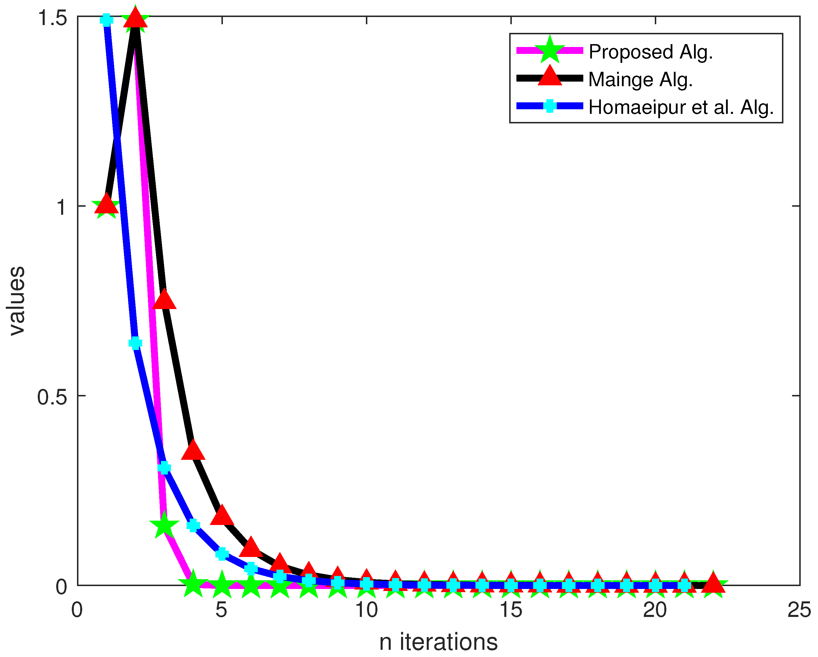
To compute and compare the results, MATLAB R2015(a) was utilized. The same initial points $(p_0,p_1)$ were used for both the proposed algorithm and Mainge’s algorithm, while for Homaeipur et al., only $p_1$ was employed. The stopping criterion for the computation was set as $|{\mathfrak{p}}_{n+1}-{\mathfrak{p}}_n|<{10}^{-10}$. The computed and compared results are presented in

Table 1. Numerical observations corresponding to the initial point $(p_0,p_1)=(0.01,0.17)$.

No. of Iterations	Proposed Alg.	Mainge [29] Alg.	Homaeipur et al. [25] Alg.
	Values	Values	Values
1	0.0147709091	0.0856800000	0.0728571429
2	0.0007829978	0.0433112323	0.0353877551
3	0.0000349538	0.0226280674	0.0180549771
4	0.0000012800	0.0120395998	0.0094573690
5	0.0000000395	0.0064811845	0.0050357419
6	0.0000000011	0.0035180150	0.0027115533
7	0.0000000000	0.0019215299	0.0014719861
8	0.0000000000	0.0010546570	0.0008040260
9	0.0000000000	0.0005811334	0.0004413075
10	0.0000000000	0.0003212466	0.0002431694

and

Table 2. Numerical observations corresponding to the initial point $(p_0,p_1)=(1,1.49)$.

No. of Iterations	Proposed Alg.	Mainge [29] Alg.	Homaeipur et al. [25] Alg.
	Values	Values	Values
1	0.1574807792	0.7475142857	0.6385714286
2	0.0027451052	0.3501328535	0.3101632653
3	0.0000725096	0.1782331851	0.1582465639
4	0.0000026469	0.0942740184	0.0828910573
5	0.0000000816	0.0506574971	0.0441367967
6	0.0000000022	0.0274787080	0.0237659675
7	0.0000000001	0.0150047930	0.0129015252
8	0.0000000000	0.0082346591	0.0070470516
9	0.0000000000	0.0045372127	0.0038679306
10	0.0000000000	0.0025080862	0.0021313087

and Figure 1 and Figure 2, respectively.

5. Conclusions

In summary, our investigation has led to several notable discoveries. The algorithm proposed in this study demonstrates robust convergence within the context of a two-uniformly convex and uniformly smooth real Banach space, featuring a relatively nonexpansive multivalued mapping. The theoretical results find support in numerical experiments conducted using Matlab R2015(a). Comparative analyses with existing algorithms, including those by Homaeipour et al. and Mainge, were performed under consistent conditions. The results, detailed in Table 1 and Table 2 and Figure 1 and Figure 2, underscore the effectiveness of our approach in terms of convergence behavior. These findings contribute valuable insights to ongoing research in optimization algorithms, highlighting the potential applicability of the proposed method in diverse contexts.

References

Alber, Y.I. Metric and generalized projection operators in Banach spaces. In Theory and Applications of Nonlinear Operators of Accretive and Monotone Type; Dekker: New York, NY, USA, 1996; pp. 15–50. [Google Scholar]
Reich, S. A weak convergence theorem for the alternating method with Bregman distances. In Theory and Applications of Nonlinear Operators of Accretive and Monotone Type; Kartsatos, A.G., Ed.; Lecture Notes in Pure and Applied Mathematics; Dekker: New York, NY, USA, 1996; Volume 178, pp. 313–318. [Google Scholar]
Mahato, N.K.; Nahak, C. Hybrid projection methods for the general variational-like inequality problems. J. Adv. Math. Stud.2013, 6, 143–158. [Google Scholar]
Preda, V.; Beldiman, M.; Batatoresou, A. On variational-like inequalities with generalized monotone mappings. In Generalized Convexity and Related Topics; Lecture Notes in Economics and Mathematical Systems; Springer: Berlin/Heidelberg, Germany, 2006; Volume 583, pp. 415–431. [Google Scholar]
Noor, M.A. General nonlinear mixed variational-like inequalities. Optimization1996, 37, 357–367. [Google Scholar] [CrossRef]
Parida, J.; Sahoo, M.; Kumar, A. A variational-like inequalitiy problem. Bull. Austral. Math. Soc.1989, 39, 225–231. [Google Scholar] [CrossRef]
Hartman, P.; Stampacchia, G. On some non-linear elliptic differential-functional equation. Acta Mathenatica1996, 115, 271–310. [Google Scholar] [CrossRef]
Blum, E.; Oettli, W. From optimization and variational inequalities to equilibrium problems. Math. Stud.1994, 63, 123–145. [Google Scholar]
Farid, M.; Cholamjiak, W.; Ali, R.; Kazmi, K.R. A new shrinking projection algorithm for a generalized mixed variational-like inequality problem and asymptotically quasi-ϕ-nonexpansive mapping in a Banach space. Rev. Real Acad. Cienc. Exactas FíSicas Nat. Ser. MatemáTicas2021, 115, 114. [Google Scholar]
Khan, M.B.; Noor, M.A.; Noor, K.I.; Chu, Y.M. Higher-Order Strongly Preinvex Fuzzy Mappings and Fuzzy Mixed Variational-Like Inequalities. Int. J. Comput. Intell.2021, 14, 1856–1870. [Google Scholar] [CrossRef]
Moudafi, A. Second order differential proximal methods for equilibrium problems. J. Inequal. Pure Appl. Math.2003, 4, 18. [Google Scholar]
Daniele, P.; Giannessi, F.; Mougeri, A. (Eds.) Equilibrium Problems and Variational Models; Nonconvex Optimization and Its Application; Kluwer Academic Publications: Norwell, MA, USA, 2003; Volume 68. [Google Scholar]
Mann, W.R. Mean value methods in iteration. Proc. Am. Math. Soc.1953, 4, 506–510. [Google Scholar] [CrossRef]
Haugazeau, Y. Sur les Inequations Variationnelles et la Minimisation de Fonctionnelles Convexes. These, Universite de Paris. 1968. Available online: https://cir.nii.ac.jp/crid/1572261550817940096 (accessed on 12 December 2023).
Nakajo, K.; Takahashi, W. Strong convergence theorems for nonexpansive mappings and nonexpansive semigroups. J. Math. Anal. Appl.2003, 279, 372–379. [Google Scholar] [CrossRef]
Matsushita, S.Y.; Takahashi, W. A strong convergence theorem for relatively nonexpansive mappings in a Banach space. J. Approx. Theory2005, 134, 257–266. [Google Scholar] [CrossRef]
Farid, M.; Irfan, S.S.; Khan, M.F.; Khan, S.A. Strong convergence of gradient projection method for generalized equilibrium problem in a Banach space. J. Inequalities Appl.2017, 2017, 297. [Google Scholar] [CrossRef] [PubMed]
Nakajo, K. Strong convergence for gradient projection method and relatively nonexpansive mappings in Banach spaces. Appl. Math. Comput.2017, 271, 251–258. [Google Scholar] [CrossRef]
Takahashi, W.; Zembayashi, K. Strong and weak convergence theorems for equilibrium problems and relatively nonexpansive mappings in Banach spaces. Nonlinear Anal.2009, 70, 45–57. [Google Scholar] [CrossRef]
Zegeye, H.; Ofoedu, E.U.; Shahzad, N. Convergence theorems for equilibrium problem, variational inequality problem and countably infinite relatively quasi-nonexpansive mappings. Appl. Math. Comput.2010, 216, 3439–3449. [Google Scholar] [CrossRef]
Markin, J.T. Continuous dependence of fixed point sets. Proc. Am. Math. Soc.1973, 38, 545–547. [Google Scholar] [CrossRef]
Górniewicz, L. Topological Fixed Point Theory of Multivalued Mappings. In Mathematics and Its Applications; Kluwer Academic: Dordrecht, The Netherlands, 1999; Volume 495. [Google Scholar]
Lim, T.C. A fixed point theorem for multivalued nonexpansive mappings in a uniformly convex Banach space. Bull. Am. Math. Soc.1974, 80, 1123–1126. [Google Scholar] [CrossRef]
Homaeipour, S.; Razani, A. Weak and strong convergence theorems for relatively nonexpansive multi-valued mappings in Banach spaces. Fixed Point Theory Appl.2011, 2011, 73. [Google Scholar] [CrossRef]
Zegeye, H.; Shahzad, N. Convergence theorems for a common point of solutions of equilibrium and fixed point of relatively nonexpansive multivalued mapping problems. Abstr. Appl. Anal.2012, 2012, 859598. [Google Scholar] [CrossRef]
Taiwo, A.; Alakoya, T.O.; Mewomo, O.T. Strong convergence theorem for fixed points of relatively nonexpansive multi-valued mappings and equilibrium problems in Banach spaces. Asian-Eur. J. Math.2021, 14, 2150137. [Google Scholar] [CrossRef]
Polyak, B.T. Some methods of speeding up the convergence of iterates methods. USSR Comput. Math. Math. Phys.1964, 4, 1–17. [Google Scholar] [CrossRef]
Maingé, P.E. Convergence theorem for inertial KM-type algorithms. J. Comput. Appl. Math.2019, 219, 223–236. [Google Scholar] [CrossRef]
Dong, Q.L.; Yuan, H.B.; Cho, Y.J.; Rassias, T.M. Modified inertial Mann algorithm and inertial CQ-algorithm for nonexpansive mappings. Optim. Lett.2018, 12, 87–102. [Google Scholar] [CrossRef]
Bot, R.I.; Csetnek, E.R.; Hendrich, C. Inertial Douglas-Rachford splitting for monotone inclusion problems. Appl. Math. Comput.2015, 256, 472–487. [Google Scholar]
Alansari, M.; Ali, R.; Farid, M. Strong convergence of an inertial iterative algorithm for variational inequality problem, generalized equilibrium problem, and fixed point problem in a Banach space. J. Inequalities Appl.2020, 2020, 42. [Google Scholar] [CrossRef]
Tan, B.; Cho, S.Y.; Yao, J.C. Accelerated inertial subgradient extragradientalgorithms with non-monotonic step sizes for equilibrium problemsand fixed point problems. J. Nonlinear Var. Anal.2022, 6, 89–122. [Google Scholar]
Farid, M.; Ali, R.; Kazmi, K.R. Inertial iterative method for a generalized mixed equilibrium, variational inequality and a fixed point problems for a family of quasi-ϕ-nonexpansive mappings. Filomat2023, 37, 6133–6150. [Google Scholar]
Zhang, Y.; Wang, Y. A new inertial iterative algorithm for splitnull point and common fixed point problems. J. Nonlinear Funct. Anal.2023, 2023, 36. [Google Scholar]
Xu, H.K. Inequalities in Banach spaces with applications. Nonlinear Anal.1991, 16, 1127–1138. [Google Scholar] [CrossRef]
Kamimura, S.; Takahashi, W. Strong convergence of a proximal-type algorithim in a Banach space. SIAM J. Optim.2002, 13, 938–945. [Google Scholar] [CrossRef]
Maingé, P.E. Strong convergence of projected subgradient methods for nonsmooth and nonstrictly convex minimization. Set-Valued Anal.2008, 16, 899–912. [Google Scholar] [CrossRef]
Schopfer, F.; Schuster, T.; Louis, A.K. An iterative regularization method for solving the split feasibility problem in Banach spaces. Inverse Probl.2008, 24, 055008. [Google Scholar] [CrossRef]
Kazmi, K.R.; Ali, R. Hybrid projection methgod for a system of unrelated generalized mixed variational-like inequality problems. Georgian Math. J.2019, 26, 63–78. [Google Scholar] [CrossRef]
Figure 1.
Producing a plot to visually depict the numerical insights outlined in Table 1 [25,29].
Figure 2.
Producing a plot to visually depict the numerical insights outlined in Table 2 [25,29].