Article

Ground Penetrating Radar in Coastal Hazard Mitigation Studies Using Deep Convolutional Neural Networks

by
Abhishek Kumar
1,
Upendra Kumar Singh
1 and
Biswajeet Pradhan
2,3,4,*
1
Department of Applied Geophysics, IIT (ISM), Dhanbad 826004, Jharkhand, India
2
Centre for Advanced Modelling and Geospatial Information Systems (CAMGIS), School of Civil and Environmental Engineering, Faculty of Engineering and IT, University of Technology Sydney, Sydney, NSW 2007, Australia
3
Center of Excellence for Climate Change Research, King Abdulaziz University, P.O. Box 80234, Jeddah 21589, Saudi Arabia
4
Earth Observation Centre, Institute of Climate Change, Universiti Kebangsaan Malaysia, Bangi 43600 UKM, Selangor, Malaysia
*
Author to whom correspondence should be addressed.
Remote Sens. 2022, 14(19), 4899; https://doi.org/10.3390/rs14194899
Submission received: 19 August 2022 / Revised: 24 September 2022 / Accepted: 27 September 2022 / Published: 30 September 2022
(This article belongs to the Special Issue Remote Sensing in Geomatics)

Abstract

:
There is a long history of coastal erosion caused by frequent storm surges in the coastal regions of Australia, which imposes great threats to communities and infrastructures alongside the beach. Old Bar Beach, New South Wales, Australia, is one such hotspot famous for its extreme coastal erosion. To apply remedial measures such as beach nourishment effectively and economically, estimating/reconstructing the subsurface hydrogeology over the coastal areas is essential. A geophysical tool such as a ground-penetrating radar (GPR) which works on the principle of reflecting electromagnetic (EM) waves, can be conveniently deployed to delineate the soil and rock profiling, water-table depth, bedrock depth, and the subsurface structural features. Here, DeepLabv3+ architecture based newly developed deep convolutional neural networks (DCNNs) were used to establish an inherent non-linear relationship between the GPR data and the EM wave velocity. The presented DCNNs have a lesser number of layers, a lesser number of trainable (learnable) parameters, a high convergence rate and, at the same time, achieve prediction accuracy comparable to that of well-established DeepLabv3+ networks, having high trainable parameters and a relatively low convergence rate. Here, firstly the DCNNs were trained and validated on small 1D datasets. Each dataset contains a 1D GPR trace and a corresponding EM velocity model. The DCNNs turned out to be quite promising in the 1D case, with training, validation, and testing accuracy of approximately 95%, 94%, and 95%, respectively. Secondly, 1D trained weights were applied to 2D synthetic GPR data for EM velocity prediction, and the accuracy of prediction achieved was approximately 95%. Seeing the excellent performance of the DCNNs in the 2D prediction case using 1D trained weights, a large amount of 1D synthetic datasets (approximately 1.2 million) were generated and gaussian noise was added to it to replicate the real field scenario. Thirdly, topographically corrected GPR data acquired over the Old Bar Beach were inverted using the DCNNs trained on 1.2 million 1D synthetic datasets to obtain the subsurface high-resolution, high-precision EM velocity, and ε r distribution information to understand the hydrogeology over the beach. The findings presented in this paper agree well with the previous hydrogeological studies carried out using GPR. Our findings show that DCNNs, along with GPR, can be successfully used in coastal environments for the quick and accurate hydrogeological investigation required for the implementation of coastal erosion mitigation methods such as beach nourishment.

1. Introduction

Coastal erosion in New South Wales (NSW) has significantly impacted private property, public infrastructure, and coastal amenities. The NSW coastline has an approximate length of 2000 km, and along this coastline, Old Bar Beach has been identified as one of the hotspots for coastal erosion [1]. Up until 2004, the Old Bar beach was receding at approximately 0.5 m/year. Since 2004, there has been a substantial acceleration in the rate of recession which at present is typically 2 m/year and, in some places, as high as 4 m/year (Old Bar Beach Coastal Protection Structure Design Investigation, 2013). In order to safeguard NSW’s coastal regions from soil erosion, numerous researchers and coastal engineers have developed many techniques [2]. Beach nourishment is one such cost-effective, efficient, and widely used technique [3]. This technique is the process of adding sediment onto or directly adjacent to an eroding beach to restore its shape. Any massive nourishment of Old Bar Beach would require a uniform increase in beach width along the entire beach embayment from Wallabi Point to Urana Bombora, a shoreline distance of approximately 4.2 km (Old Bar Beach Coastal Protection Structure Design Investigation report, 2013). Sand volumes required to nourish Old Bar Beach are estimated to be in the order of 1,000,000 m3 initially, with subsequent nourishment campaigns of roughly 1,000,000 m3 required approximately every 10 years. The total cost to implement such a scheme is estimated at AUD 147.1 million (Old Bar Beach Coastal Protection Structure Design Investigation report, 2013). To implement this technique effectively and economically, it is crucial to accurately map the rock basement to estimate potential storm sediment mobilization and delineate the water table and other near subsurface geological structures. The ground penetrating radar (GPR) geophysical method can play an important role in the effective implementation of coastal erosion mitigation techniques [4].
Ground Penetrating Radar (GPR) is a non-destructive near-surface geophysical tool and a high-resolution image producer, which is extensively used in the fields of glaciological investigation [5], archaeological investigation [6], and civil and geotechnical investigation [7]. GPR works on the reflection principle of electromagnetic (EM) waves [8], sends EM pulses into the ground, and records the two-way travel time (TWTT) and amplitude of the reflected signals. Reflection of EM pulses occurs due to the presence of subsurface relative dielectric permittivity ( ε r ) contrast. EM velocity maps inverted from the recorded GPR data by geophysical nonlinear inverse modeling can be conveniently used for the reconstruction of the sediment thickness, water table, and other near-subsurface geological features. This reconstruction of the subsurface requires a good initial guess value of the Earth’s physical properties and knowledge of physical equations or theories [9,10]. Machine learning (ML) techniques can be applied efficiently and effectively without prior knowledge to solve the ill-posed and nonlinear inverse problems [9].
Recently, deep learning (DL), which is a part of ML, has gained appeal in many scientific disciplines due to its notable successes in image classification with excellent accuracy [11], prospective mineral mapping [12], automatic interpretation of seismic data [13], geological fault detection [14], and estimation of the 2D velocity model for oil and gas exploration directly from unprocessed multiple seismic offsets seismic data [15,16,17]. Some researchers have applied deep learning along with transfer learning [18] and Genetic Adversarial Networks (GANs) [19] to enhance the feature detection power, resolution, and precision of Convolutional Neural Networks (CNNs) for application to GPR data. Application of deep learning has also been seen in natural hazards areas such as landslides modeling, floods modeling, and forest fires mapping [20,21,22] with satisfactory results. However, very few studies demonstrate that DL helps in the successful implementation of coastal hazard mitigation strategies by obtaining the distribution of physical properties such as EM velocity in the Earth’s near subsurface using GPR data [4]. Obtaining a high-resolution, high-precision subsurface EM velocity map from GPR data for hydrogeological studies requires a robust technique.
In our research, we have attempted to introduce an innovative DeepLabv3+ based [23] new Deep Convolutional Neural Network (DCNNs) and trained it with a significant amount of 1D synthetic datasets containing GPR traces (input) and EM velocity models (output). DCNNs learn the hidden non-linear relationship between the input and the output data and predict velocity models based on their learning when it encounters new GPR data. The subsurface structure complexity, mechanics of wave propagation, and source wavelet employed for generating synthetic data are all factors that can influence the regression process between GPR traces and the EM velocity models. Here, selecting a good initial value of the physical properties/parameters is not crucial since the presented DCNNs have been trained with a wide range of synthetic EM velocity models and corresponding GPR traces, which cover all widely-accepted geological knowledge [8]. This research has highlighted the potential of GPR and the robustness of our DCNNs in the effective implementation of coastal erosion mitigation strategies.
The DeepLabv3+ architecture, which Google has invented, is the latest extension of previous versions of the DeepLab series. DeepLabv3+ is a semantic segmentation architecture that builds on DeepLabv3 [24] by adding an effective decoder module to enhance segmentation results. DeepLabv3+ has rich semantic knowledge in the encoder module, and the decoder module obtains the detailed object boundaries [23]. Atrous Spatial Pyramid Pooling (ASPP) [24], available in DeepLabv3+, investigates an incoming convolutional feature layer with filters that contain dilation rates and so its effective field of view continues to increase, thus capturing objects and image context at multiple scales. Our novel DCNNs also have an effective encoder–decoder module with a smaller number of layers, well-tuned hyperparameters, and ASPP (dilated filter) in the decoder part. All these factors reduce the number of trainable parameters of our DCNN, which makes it computationally faster (shorter training time), highly convergent, and at the same time, it achieves prediction accuracy comparable to the accuracy achieved by existing DeepLabv3+ based neural networks with a higher number of layers, a higher number of trainable parameters, and a relatively low convergence rate.
Based on the excellent accuracy of our innovative DCNNs in predicting EM velocity and ε r from 1D and 2D synthetic GPR data, the DCNNs were trained on large synthetic 1D datasets (over 1.2 million) and applied to common-offset, topographically corrected field GPR data acquired over the Old Bar Beach, New South Wales, Australia [25]. The predicted EM velocity maps and ε r distribution plots were analyzed to identify different subsurface hydrogeological features. We estimated and characterized the smallest and the largest thickness of the sediment, the water table depth, location of former cut and fill channels, and other geological features using predicted high resolution, high precision EM velocity maps, and ε r distribution plots. Our findings are well matched with the available geological and geophysical samples (Old Bar Beach Coastal Protection Structure Design Investigation report, 2013, appendix D) of this area [25]. The DL technique presented in this paper will be very useful in the quick hydrogeological investigation for the effective and economical implementation of coastal erosion mitigation techniques. These studies can be further carried out to improve the resolving power of our DCNNs by training them with even larger synthetic datasets covering a wider range of geological material properties so that thin beds such as seaward-dipping reflectors, basal reflectors which are frequently seen in coastal sedimentary environments, can be identified in predicted EM velocity maps. Knowledge regarding these thin beds is important from a coastal erosion studies point of view.

2. Methodology

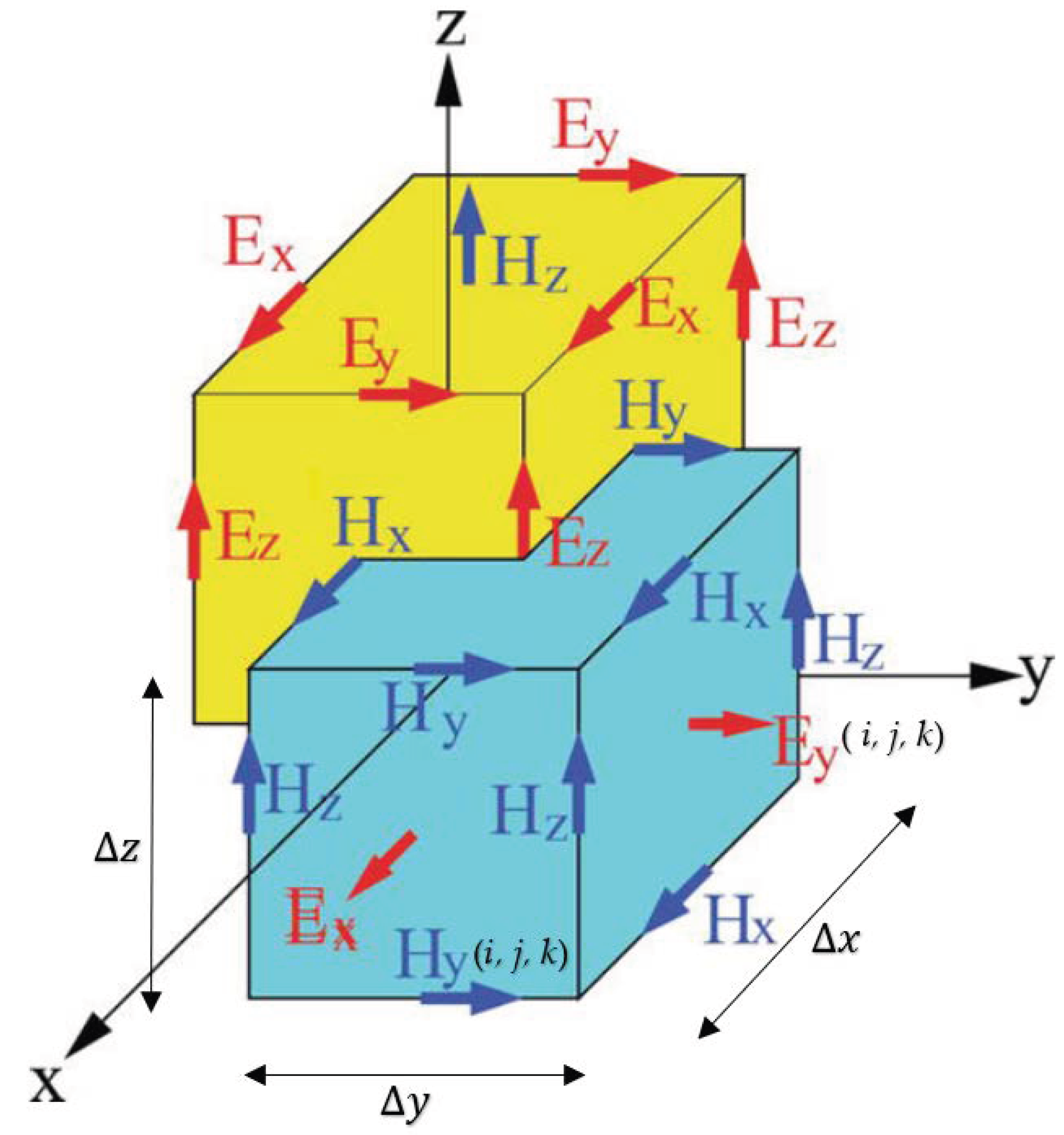
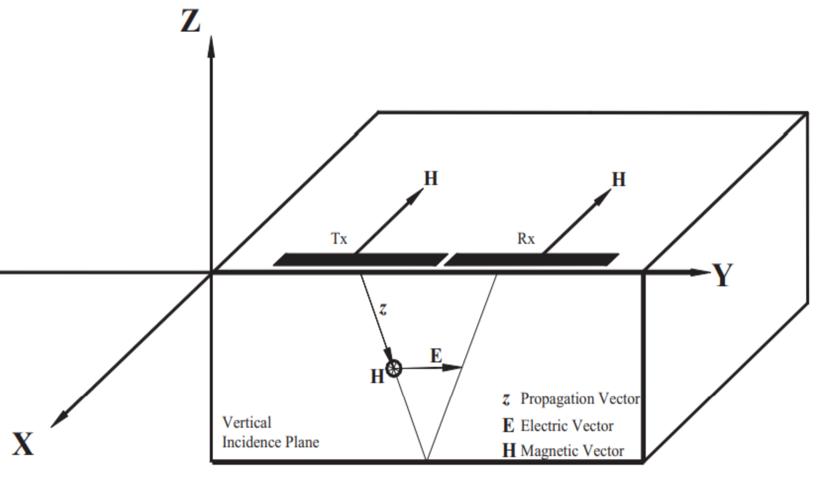
2.1. Forward Modeling

First, a number of random 1D EM velocity models are generated using a certain EM velocity range. The range of velocity should be selected in such a way that it incorporates all common geological materials [8]. From these 1D velocity models, ε r are obtained using the Equation (1) as shown below:
ε r = c v 2 ,
where c is the speed of light and v is the velocity of the EM wave in the subsurface. Then, the finite difference time domain (FDTD) algorithm [26] is used to carry out forward data modeling to generate GPR traces using   ε r and adopting a setup with offset as zero between source and receiver. Equations (2)–(5) are called Maxwell’s equations [8] which are very important in understanding the behavior of GPR because the connection between electromagnetic properties of materials and the propagation of EM waves through materials can be quantitatively explained using Maxwell’s equations as shown below:
¯ × E ¯ = B ¯ t ,
¯ × H ¯ = J ¯ + D ¯ t ,
¯   .   D ¯ = q ,
¯   .   B ¯ = 0 .  
Here, E is a vector denoting the strength of the electric field, B is a vector denoting the density of magnetic flux, electric displacement is denoted by a vector D, the intensity of the magnetic field is denoted by H, electric charge density is denoted by q, and the density of the electric current is denoted by vector J. In Equations (2) and (3), magnetic flux density vector (B) and electric displacement vector (D) are in partial differential form with respect to time (t). Basically, Maxwell’s equations explain the behavior of electric and magnetic fields and how they are interrelated. The FDTD method provides the direct integration of Maxwell’s time-dependent equations. Equations (6)–(13) are governing equations [26] in the FDTD algorithm.
× E = i ω μ H ,
× H = σ E + i ω ε r E .
ε r ,   μ , and σ denote the relative dielectric permittivity, magnetic permeability, and electrical conductivity, respectively. Angular frequency is denoted by ω , and the operator has the following form:
= x   1 s x x + y   1 s y y + z 1 s z z ,  
where
s k = K k + σ k α k + i w ε 0 ,   k = x , y , z .
Here, s k are complex coordinate stretched variables that changes only in the k direction [27]. ε 0 is the absolute dielectric permittivity in free space and σ k , K k , and α k are the parameters which permit the propagation of a wave inside the modeling grid and propagation of a wave in the boundary regions of a perfectly matched layer (PML) [28]. One should note that σ k , K k , and α k are not true indicators of electrical properties. These are parameters which add an extra degree of freedom (DOF) to equations of Maxwell through the stretching of complex coordinates for the implementation of the PML boundary. On finding the values of Equations (6) and (7) using the identity provided in Equation (8), and with an assumption that for 2D modeling, there is no change in the y direction, the three sets of Equation (10a–c) involving the [ H X , H Z , E Y ] and [ E X , E Z , H Y ] field components (Figure 1) in the partial differential form are obtained and can be stated in the following forms:
i ω μ H x = 1 s z E y Z ,
i ω μ H z = 1 s x E y x ,
σ E y + i ω μ E y = 1 s x   H Z x 1 s z   H x z .
On taking the inverse Fourier transform of the inverse of Equation (9), we obtain an Equation (11).
s k 1 t = δ t K k σ k ε 0 k k 2 exp t ε 0 σ k K k + α k u t = δ t K k + δ z t ,
where δ z t   = σ k ε 0 k k 2 exp t ε 0 σ k K k + α k u t . Here, δ t is the Dirac delta function [26], and u t is the Heaviside step function [26]. Here, t denotes time.
Equation (10a–c) are the transverse magnetic (TM) mode sets of equations. In the TM polarization mode of GPR data acquisition, polarization has an orientation of E within a vertical plane which is parallel to the incidence plane (Figure 2). In Figure 2, the electric field vector (E) is parallel to the Z−Y plane, which is an incident plane and perpendicular to the X−Z plane. Here, Y is the direction of measurements. Using the expression in Equation (11) and by assuming that material properties are independent of frequency, Equation (10a–c) are converted into the time domain as follows:
μ H x t = 1 k z E y Z δ z t *   E y Z .
Equation (12) represents Equation (10a) in the time domain. In the same way, equations in the time domain for (10b,c) can be written. Here, * represents convolution. Equation (12) is approximated using finite-difference for TM mode modeling of GPR using the following equation:
  H x | i j + 1 2 n + 1 2 = H x | i j + 1 2 n 1 2   D b z | i j + 1 2 E y | i j + 2 n + 27 E y | i j + 1 n 27 E y | i j n + E y | i j 1 n D c | i j + 1 2 τ H x z | i j + 1 2 n .  
In Equation (13), the subscripts denote the spatial position, and the superscripts denote time (i.e.,     H x | i j + 1 2 n + 1 2 represents the   H x component of the magnetic field at position (x, z) = i Δ x , j + 1 / 2 Δ z ) and time n + 1 2 Δ t . Here, Δ x and Δ z are discretization intervals in the EM field in the horizontal and the vertical direction, and Δ t denotes the time step). FDTD modeling is accomplished using these equations and alternately updating the electric and magnetic fields. Here, D c =   Δ t / μ . In Equation (13), D b z is the coefficient which is specified in terms of grid parameters and electrical properties. After obtaining the [ H X , H Z , E Y ] and [ E X , E Z , H Y ] field components, these components are placed in the Yee lattice in a certain orientation, as shown in Figure 1. This leads to the generation of an EM field which propagates the EM waves to generate GPR traces.

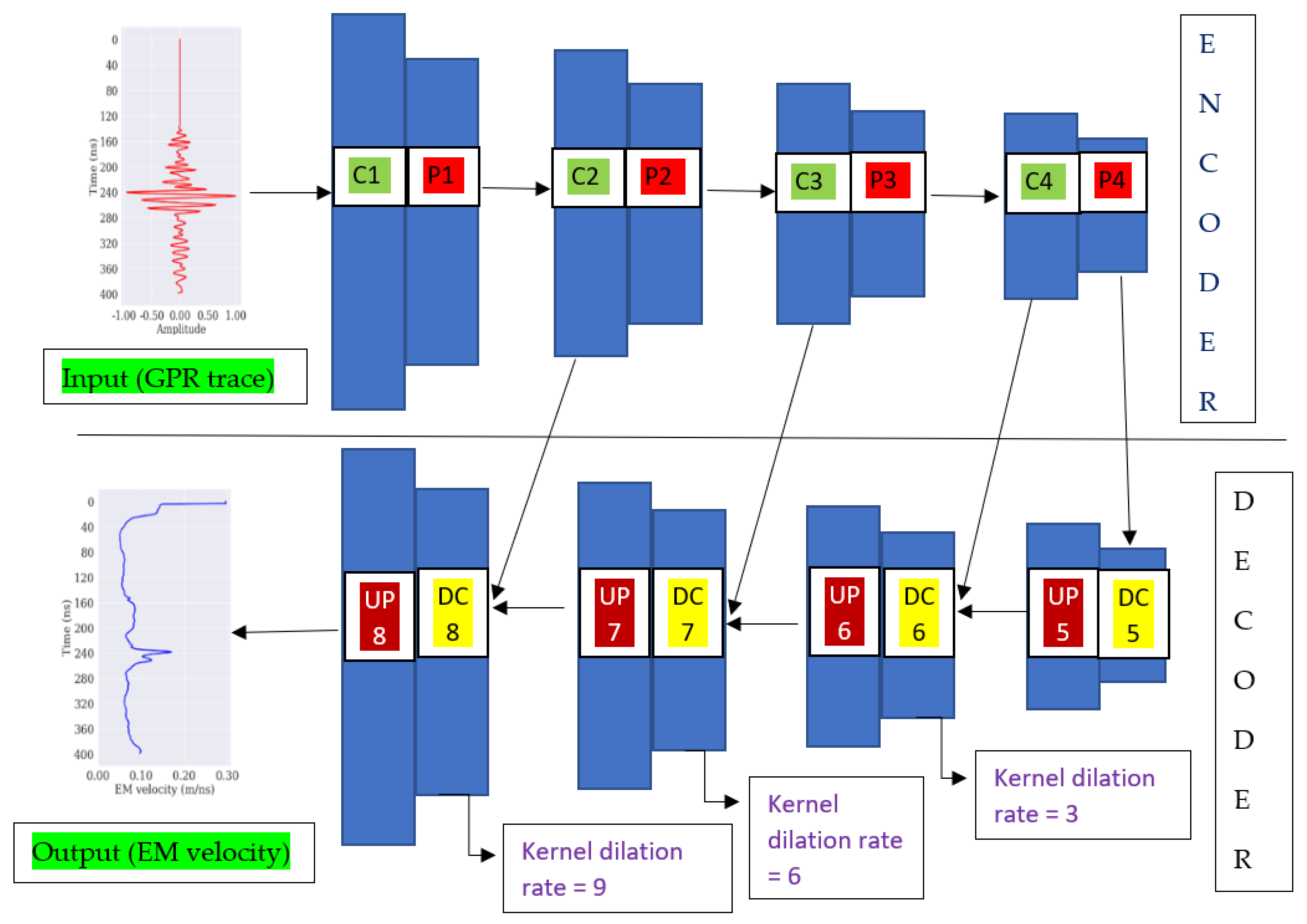
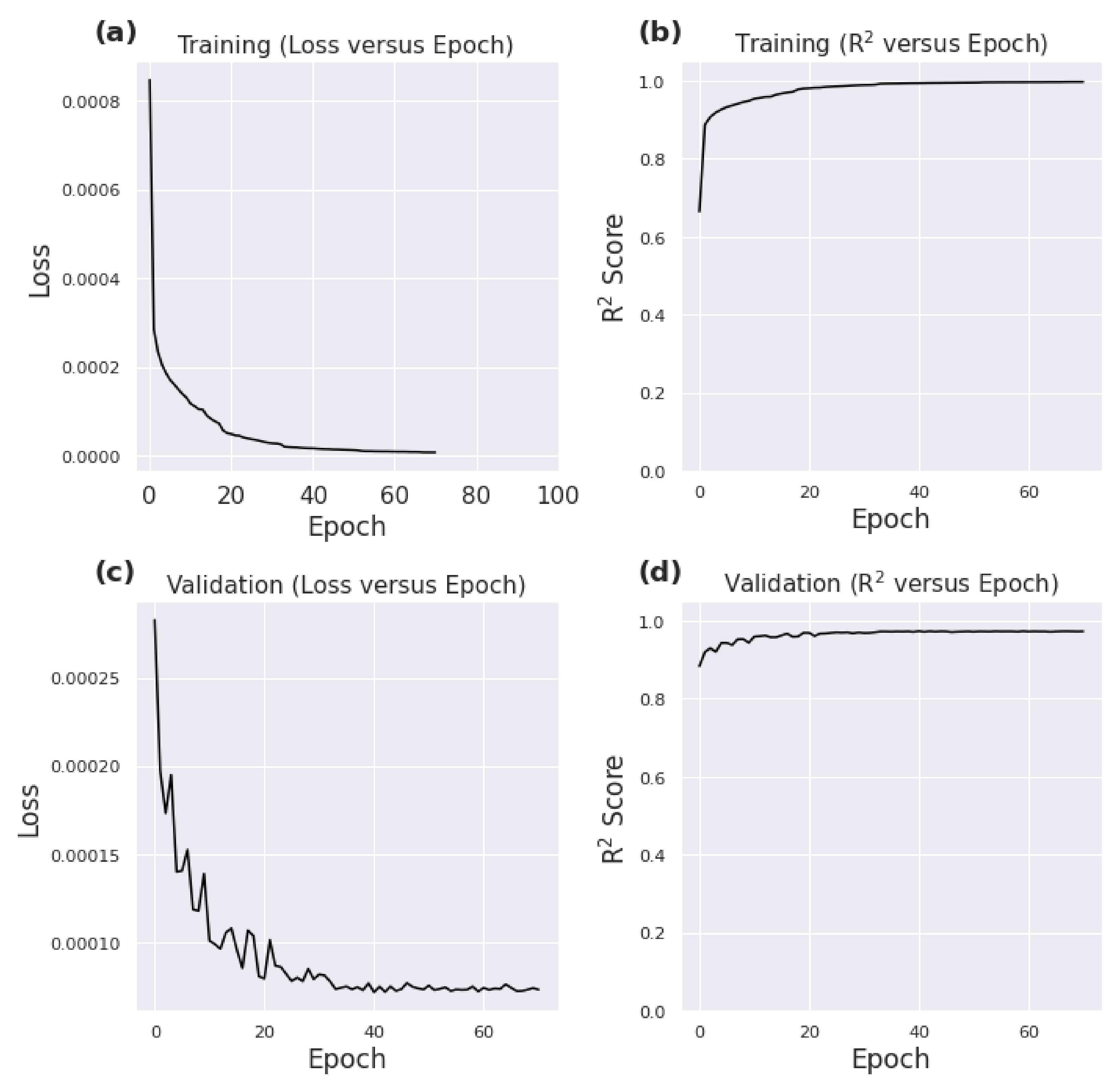
2.2. Inverse Modeling: Deep Convolutional Neural Networks (DCNNs)

DeepLabv3+ is an architecture that performs better than many state-of-the-art picture segmentation architectures, as suggested by ref. [30]. DeepLabv3+ is a semantic segmentation architecture. Semantic segmentation-based algorithms are outstanding at learning the underlying relationship between parameters with the same domain [30]. Here, input data (GPR) and its output (EM velocity) taken for training the DCNNs are in the same domain, i.e., time. On the next page, Figure 3 illustrates our DeepLabv3+ based developed DCNNs, which are part of an encoder–decoder system and have atrous convolution (dilated filter) in the decoder part. The encoder captures inherent information in the input data, and the decoder interprets the encrypted information to generate the output model. We tuned the hyperparameters (number of layers, number of filters, size of filters, filter dilation rate) of our DeepLabv3+ based DCNNs in order to reduce the number of trainable parameters and, at the same time, maintaining good prediction accuracy. The total number of trainable parameters in our tuned DCNN is 1,287,769, which is lesser than the trainable parameters of DeepLabv3+ based recent networks such as GPRNet [30]. GPRNet has a total of 1,392,585 trainable parameters [30]. Lesser trainable parameters make our tuned DCNNs computationally fast during the training process, which saves time and, at the same time, achieves good prediction accuracy. Our tuned DCNNs also have a high convergence rate compared to GPRNet. By high convergence rate, we mean that our tuned DCNNs can reduce the loss significantly during training in a lesser number of epochs (iterations) which GPRNet is achieving in a greater number of epochs.
Table 1, shown on the next page, illustrates the comparison of the GPRNet (2nd column), with developed DCNNs having the same values for hyperparameters as GPRNet (3rd column), and with DCNNs having its hyperparameters tuned to reduce trainable parameters and increase the convergence rate (4th column). The parameters considered for comparison include the number of layers, hyperparameters values and optimizer, number of trainable parameters, number of convergence epochs, loss reduction, accuracy in 1D and 2D synthetic EM velocity prediction, and training duration. We used the same synthetic 1D datasets for training all three versions of neural networks to evaluate these parameters. Table 1 shows DCNNs with the same values for hyperparameters that GPRNet has, providing excellent accuracy in 1D and 2D EM velocity prediction, but they have high trainable parameters (4,765,961) and low convergence rates, which make them computationally slower (longer training time) and inefficient in today’s scenario where saving time is important. Our aim is to use a DeepLabv3+ based neural networks which have lesser trainable parameters, a high convergence rate, and, at the same time, maintains good prediction accuracy. Tuned DCNNs turned out to be the best choice for us after considering all comparison parameters.
In Figure 3, the input to DCNNs is a GPR trace, and the output is an EM velocity model. C and P indicate 1D convolution and 1D max pooling layers, respectively. DC and UP indicate 1D deconvolution and 1D up-sampling layers, respectively. There are 16 layers in the network, which includes 4 convolution layers, 4 max-pooling layers, 4 deconvolution layers, and 4 up-sampling layers. In the decoder part, the input to deconvolution (DC) layer numbers 6, 7, and 8 are being fed by merging the outputs of convolution (C) layer numbers 2, 3, and 4 with outputs of up-sampling (UP) layer numbers 5, 6, and 7. The kernel dilation rate in the decoder part varies from 3 to 9. The kernel is also known as a filter. The input data is encoded into basic feature building blocks at each epoch in the encoder, and the decoder reconstructs the model (output) from basic feature building blocks. Backpropagation is used to update the training weights while regressing between the input data and output model for several iterations, with the objective function being minimized until convergence. Convolution layers extract features from GPR data (input) by performing 1D convolution by moving a filter onto itself, which acts as a feature detector. One-dimensional max-pooling layers minimize the incoming data dimension while preserving important information contained in the incoming data. With each consecutive DC layer, the number of filters in the layer decreases. UP layers apply 1D up-sampling to the input layers, producing an output of the same length as the input. In our DCNNs, Padding was set to “same” throughout the network so that the input data and output model size remained the same. The activation layer used is Rectified Linear Unit (ReLu) [31]. The adaptive moment estimation (ADAM) algorithm [32] was used as an optimization approach. ADAM is efficient for stochastic optimization, requiring only first-order gradients with little memory requirement. ADAM computes individual adaptive learning rates for different parameters from estimates of the first and second moments of the gradients. Here, mean squared error (MSE) [33] has been used as an objective function.

2.3. Workflow for Inversion Using DCNNs

Firstly, to check the robustness of our tuned DCNNs in predicting accurate EM velocity, they were trained with a small dataset containing 9800 1D synthetic GPR traces and corresponding 1D EM velocity models. DCNNs training was accomplished using a high-performance computing facility with two Intel Xeon [email protected] processors and 192 GB DDR4-2933 RAM available at IIT(ISM), Dhanbad, Jharkhand, India. Secondly, velocity prediction on synthetic 1D zero-offset GPR testing datasets was performed using saved model weights before moving on to 2D space. EM velocity prediction results in the case of 1D testing datasets turned out to be very successful, with prediction accuracy up to ( R 2 ) 99%. Accuracy was measured in terms of the coefficient of correlation ( R 2 ). R 2 is a statistical measure of the degree to which change to the value of one variable (GPR trace) predicts the change to the value of another (EM velocity model). R 2 is expressed as values between +1 and −1. Thirdly, using weights of DCNNs trained with 1D datasets, 2D EM velocity model prediction was performed on 2D synthetic GPR data with prediction accuracy up to 95%. Seeing the excellent performance of DCNNs trained with a small 1D datasets in EM velocity prediction from 2D synthetic GPR data, a huge number of datasets containing approximately 1.2 million 1D GPR traces and corresponding EM velocity models were generated to train the DCNNs. Gaussian noise (0.15σ–0.85σ, where σ is the standard deviation of the individual trace of GPR) was added to it to replicate the real field scenario as field data are noisy. Fourthly, the model weights of DCNNs trained with the large datasets were applied to topographically corrected field GPR data acquired over Old Bar Beach, NSW, Australia, to predict the subsurface distribution of EM velocity and relative dielectric permittivity ( ε r ) .

3. Simulated Examples

3.1. Generating the Synthetic GPR Data

The presented DCNNs were trained using synthetic datasets generated by adopting a broad range of EM velocity to establish a better relationship between the input data (GPR traces) and the output data (EM velocity model). Velocity models ranging from 0.048 to 0.175 m/ns were generated to simulate 1D GPR traces. This velocity range corresponds to the relative dielectric permittivity values of 3 to 39 [8]. This velocity range was chosen since it encompasses the most common geological materials [8,34]. Moreover, the velocities for 4 to 15 layered systems were also generated. Both sets of velocity models were combined. The combined set of velocity models is in the spatial domain and converted to the time domain using Equation (14) shown below:
v = 2 h T ,
where h is the layer thickness, and T is the two-way travel time (TWTT) within the layer. Then, 1D GPR traces were created from corresponding velocities with a zero-offset arrangement in the 2D FDTD scheme. The source wavelet taken here in the FDTD scheme is the Ricker source wavelet [35]. This wavelet is noncausal and symmetric regarding its origin time. One important quality the Ricker wavelet has is that it is a zero-phase signal [36]. In continuous time, the second derivative of the Gaussian function provides the Ricker wavelet. The Ricker source wavelet also provides a good representation of many commercial GPR instruments and a good amount of desired bandwidth for geo radar applications [36,37]. To retain the same forward modeling solver, the 2D FDTD method was employed to generate 1D GPR traces so that the model weights of DCNNs trained with 1D datasets can be tested on 2D synthetic GPR data for EM velocity prediction. With parallel computing, the computational cost of forward data modeling is relatively cheap. Simulating 10,000 GPR traces from 10,000 velocity models took less than an hour using a high-performance computing facility with two Intel Xeon Gold [email protected] GHz processors and 192 GB DDR4-2933 RAM available at IIT(ISM), Dhanbad, Jharkhand, India.

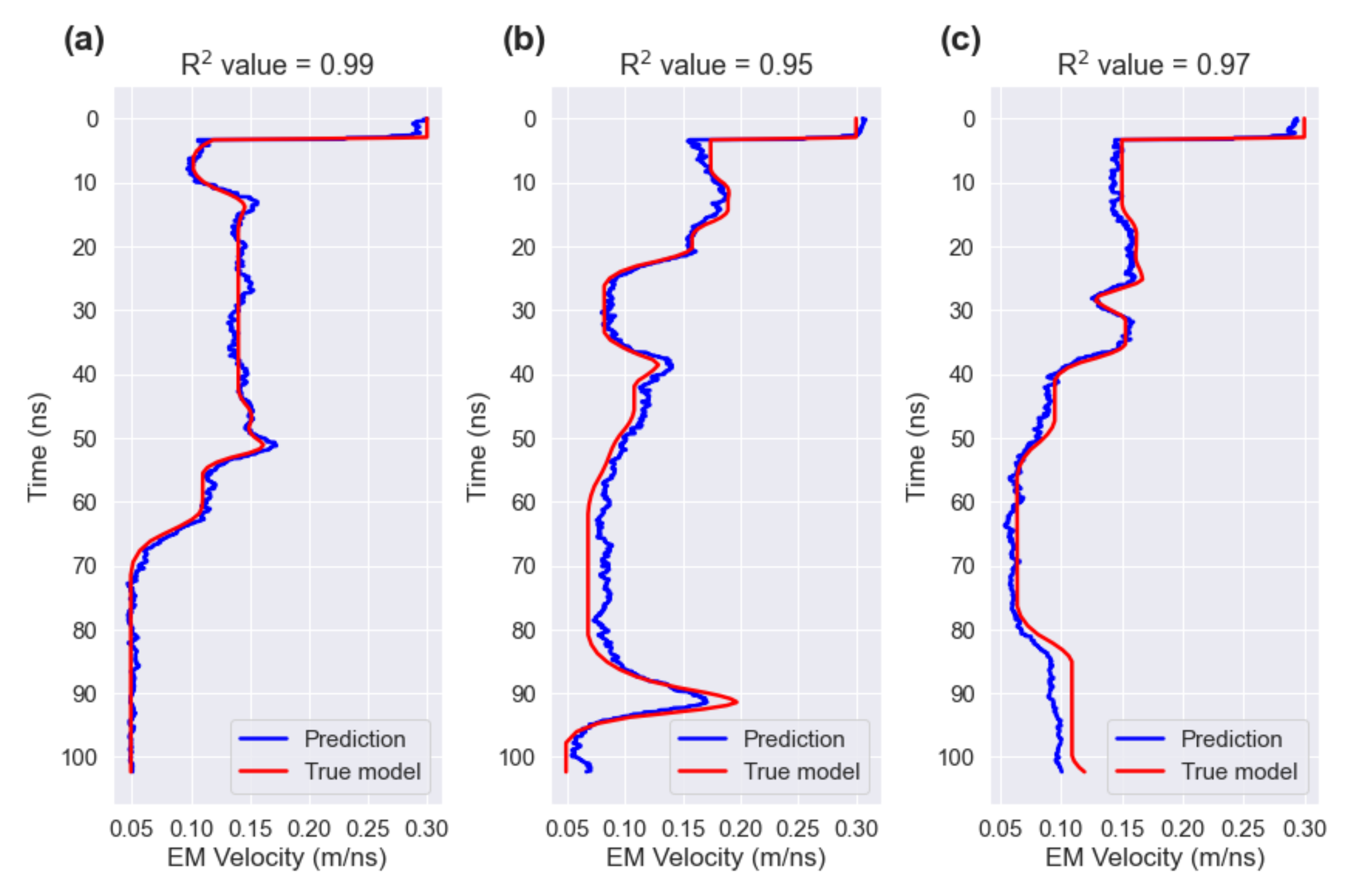
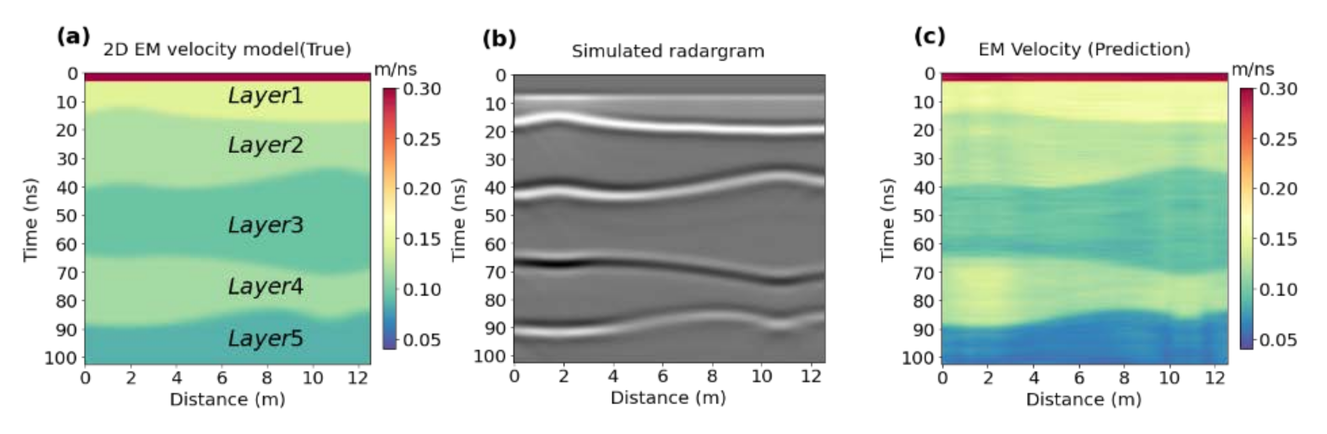
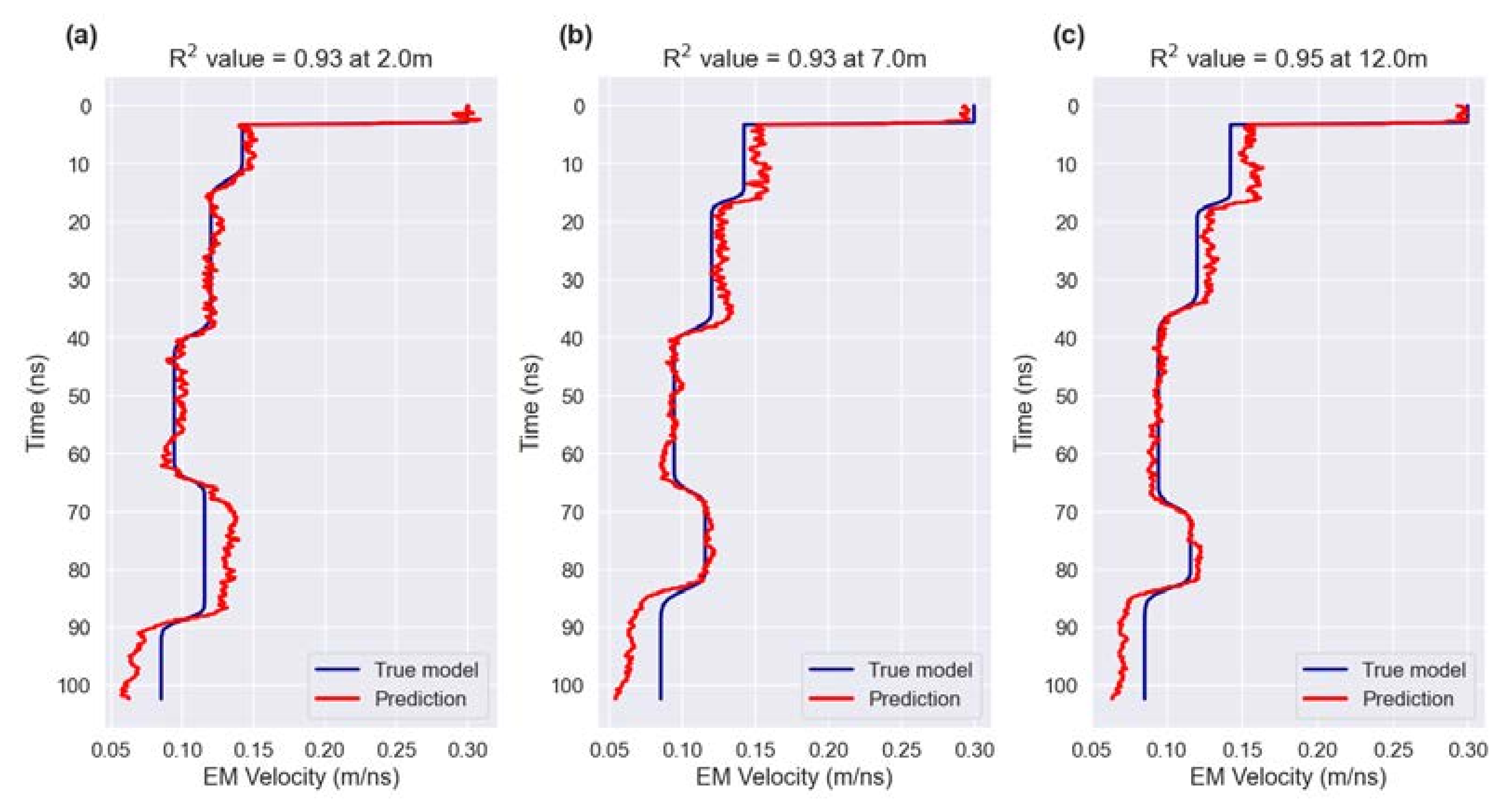
3.2. Application of DCNNs to 1D/2D Synthetic GPR Data

Before training the DCNNs, direct waves were removed from the 10,000 generated synthetic GPR traces, and a maximum normalization scheme was applied to them. The max normalization scheme normalizes the amplitude values of GPR traces individually based on the maximum amplitude of each GPR trace. In total, 10,000 1D datasets were prepared, with 1% (100) retained for validation, 1% (100) retained for testing, and the remaining 98% (9800) being used to train the DCNNs. Each dataset includes a GPR trace as well as a corresponding velocity model. The data used to train the DCNNs has an array length of 1280 nanoseconds (ns). This 1280 ns array length denotes the TWTT (Y-axis) of GPR traces. The kernel size k was set to 12, while the number of filters n was initially set to 12. The number of filters continued to increase in the encoder part and decreased in the decoder part. DCNNs were trained by supplying data in mini batches of 40. The “Early stopping” option was used in the training of DCNNs, which stopped the training process if validation accuracy did not change during the given value of “patience,” which was set as 30 epochs in our algorithm. Patience is the number of epochs during which there is no improvement in the monitored model parameter. The training and validation converged at epoch 71. The training loss, training accuracy, validation loss, and validation accuracy plots are shown in Figure 4a–d, respectively. DCNNs took around 1.5 h (hours) to become trained.
Three random GPR traces from the testing dataset were selected to predict velocity models using the 1D trained weights, and matching results are shown in Figure 5a–c.
Figure 5 shows that the prediction results are reliable, with maximum R 2   values of 0.99 for randomly chosen GPR traces from the 1D testing dataset. As seen in Figure 5, it can be said here that the training of DCNNs is able to establish a relationship between the input data (GPR) and the output model (EM velocity) and allows us to outstand the accuracy while predicting outputs. The predicted velocity models are comparable to the true models. Since the velocity prediction in the 1D case is reasonably accurate, motivation was drawn to apply the trained 1D model weights on 2D synthetic GPR data to predict the 2D EM velocity model. A five-layered simple 2D velocity model was created with velocities of 0.14, 0.12, 0.09, 0.11, and 0.09 m/ns for layer 1, layer 2, layer 3, layer 4, and layer 5, respectively, as shown in Figure 6a. These EM velocity values in the 2D velocity model correspond to various geological materials [8]. Firstly, the 2D FDTD algorithm was applied to the 2D velocity model to collect the whole common offset shot traces. The 2D GPR data were then created by horizontally stacking the traces nearest to the appropriate sources (Figure 6b). In FDTD, the distance between the source and the receiver was kept at 5 cm. Overall, 12.55 m was the model’s horizontal distance. Figure 6c shows the predicted 2D velocity model obtained by applying model weights of DCNNs trained with 1D datasets.
While certain artifacts were introduced in Figure 6c, the geometry and shape of each stratum remained mostly unchanged from the true model shown in Figure 6a. The accuracy of three 1D velocity models picked up at different offsets from the 2D predicted velocity model (Figure 6c) were compared with their associated true velocity models (Figure 6a). It was found that the predicted velocity models are well-matched with the true models (Figure 7a–c), in which R 2 values are 0.93 at 2.0 m offset, 0.93 at 7.0 m offset, and 0.95 at 12.0m offset. It clearly shows that our DCNNs, which were trained with 1D datasets, can predict the EM velocity from 2D GPR data with great accuracy. Therefore, to apply our DCNNs to field GPR data, which are usually in the 2D form, the DCNNs were trained with a huge number of 1D synthetic datasets covering a wider range of geological material properties.

4. Field Examples

The excellent accuracy of DCNNs-based prediction of EM velocity from 2D synthetic GPR data provided the motivation to investigate the relevance of our DCNNs in the inversion of field GPR data acquired in coastal environments for the implementation of coastal erosion mitigation techniques. For field application, GPR data acquired from the Old Bar Beach, NSW mid-north coast (between Newcastle and Port Macquarie), South Australia [25] have been used. The main purpose of the collection of GPR data over the study area was to estimate the least and the largest thickness of the sediment, depth of water table, depth to any competent substrate or pre-holocene surface that might reduce the strength of water waves causing coastal erosion, location of former channels, and to identify other subsurface geological features. Some researchers have suggested that the estimation of water table depth over the coastal area is important as there is a direct relationship between the water table depth and coastal erosion of the beach [38]. The water table closer to the ground surface promotes foreshore erosion, while the water table at greater depth retards erosion and promotes dune formation [38]. However, it has also been seen that the one-in-one relationship between the beach water table depth and coastal erosion, as suggested by ref. [38], is not supported by a large majority of the coastal morphologists. Dune formation is promoted, especially with a wide (and dry) beach. Some researchers have promoted beach drainage (i.e., lowering the groundwater table artificially) as a means to decrease erosion, but practical tests showed that this method did not work. Much more relevant is the location of former channels, which can also be found with the deep learning technique illustrated in this paper. Our DCNNs based predicted subsurface EM velocity maps and relative dielectric permittivity ( ε r ) distribution information can enable the implementation of coastal erosion mitigation techniques such as beach nourishment in more economical and effective way by providing a more accurate thickness of sediment and the location of different hydrogeological features so that coastal engineers and researchers can know exactly where they must add more sand or less sand in order to restore the shape of the beach which was deformed due to coastal erosion.

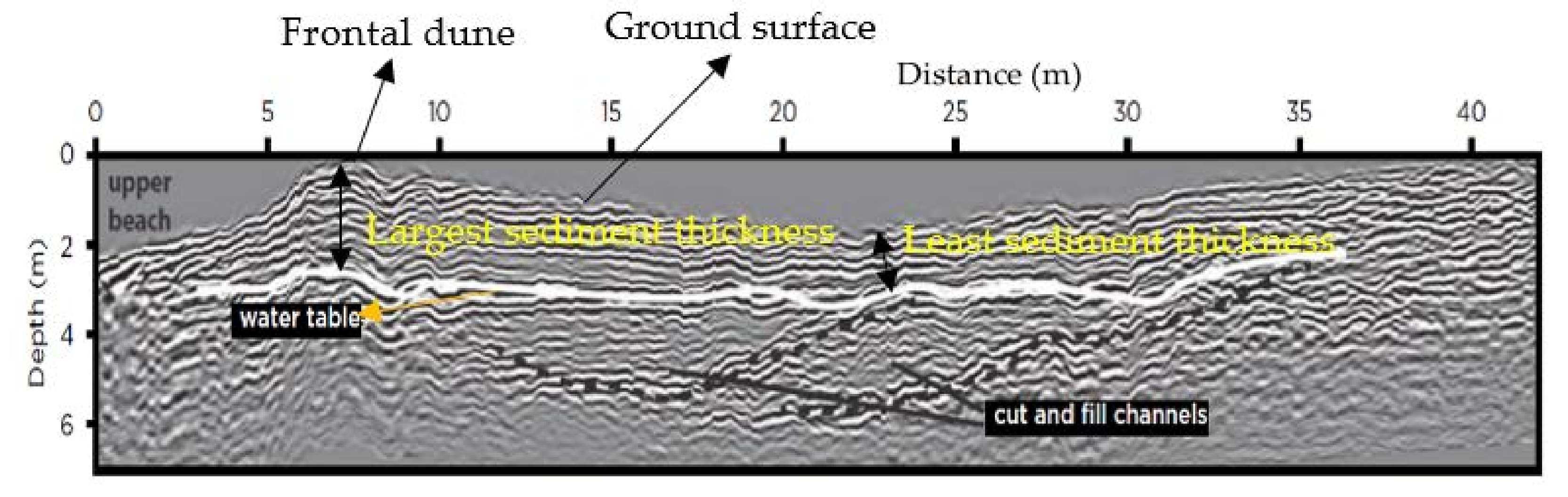
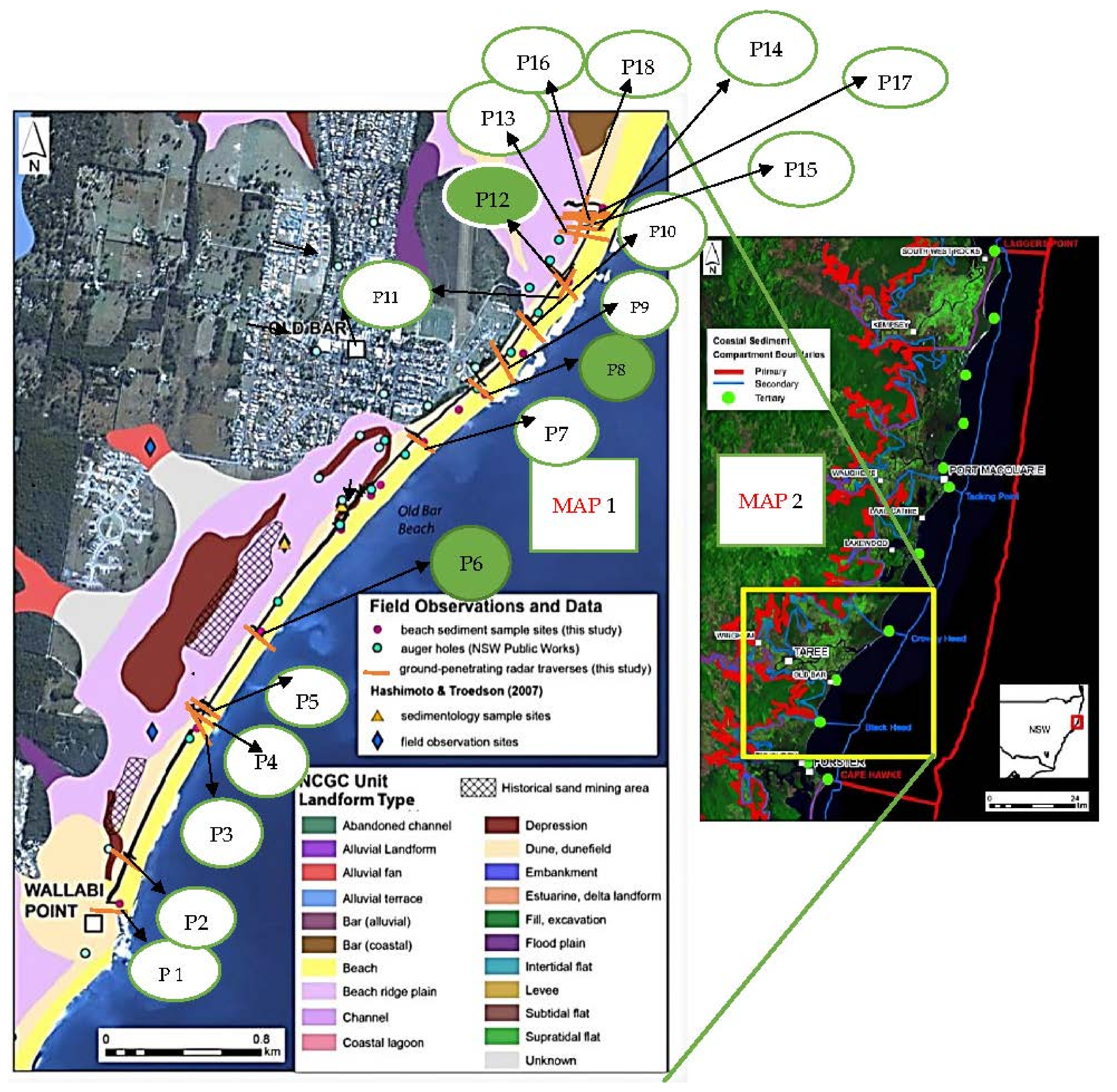
4.1. Description of the Field Data

On Old Bar Beach, GPR data were collected from over 18 locations from the 2nd to 5th March 2015 [25]. A MALA Pro-Ex GPR system with a 250 MHz shielded antenna was used to collect the data. In this paper, GPR data acquired over three locations were inverted using the trained DCNNs. The topographically corrected processed form of GPR data shown in Figure 8 was acquired from one location [25] and has a profile length of 45 m and 7 m as the depth of investigation. The GPR data shown in Figure 8 were studied and analyzed by previous researchers, and different hydrogeological features were identified by them [25]. According to them, the water table is between 3 m to 4 m in depth [25]. The cut and fill channels shown with dotted lines are between 4 m to 6 m in depth [25]. In this paper, complete analysis was performed for the GPR data shown in Figure 8 using our DCNNs. A total of 587 traces were collected for the GPR profile shown in Figure 8 [25]. For the other two sets of GPR data, only the raw GPR data, processed GPR data, and its DCNNs-based inverted velocity models in the time and depth domain were discussed in this paper. All GPR data were acquired within a geographical bounding box with coordinates 152.54°, −32.35°, 152.60°, and −31.97° for west longitude, south latitude, east longitude, and north latitude, respectively [25]. All three GPR data analyzed in this paper have profile orientation perpendicular to the surface water line [25].

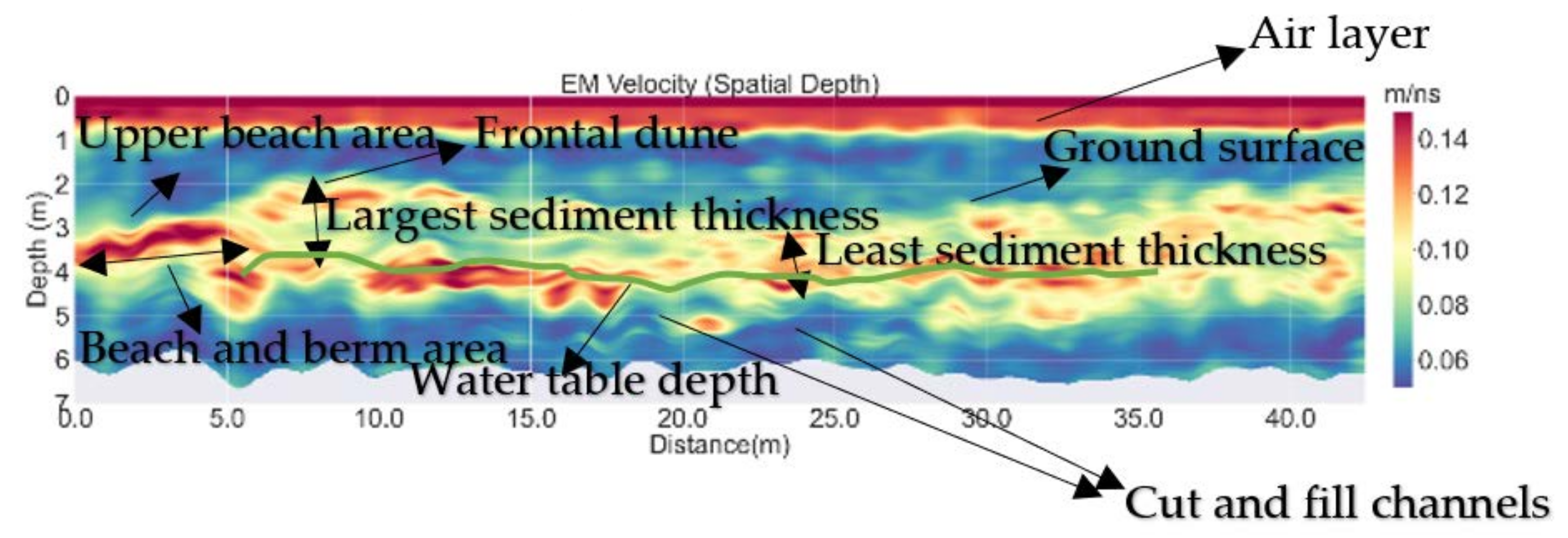
4.2. Coastal Sediment Compartment Boundaries and Landform Types

Coastal erosion and shoreline recession due to rising sea-levels seriously threaten Australia’s coastal areas. Individuals, corporations, and local governments have conducted coastal risk assessments to learn how they may be impacted now and in the future. The coastal sediment compartment boundaries and landform types (Figure 9) project in New South Wales intends to assist users in conducting or commissioning best-practice risk and erosion assessments based on the physical characteristics of the coastal environment using a uniform approach [39]. As a result of this approach, evaluations may be easily compared to neighboring locations or scaled up to fit inside broader regional assessments. Australia’s southeast coastline (NSW) has been divided into three coastal compartments based on landforms and sediment (sand and beach subsurface geology) migration patterns, as shown in Figure 9. The three coastal compartments are as follows: (a) the primary compartment is based on big landforms and offshore processes that are ideal for regional planning or large-scale engineering such as ports, bridges, high-rise buildings, etc., (b) the secondary compartment is based on medium landforms and regional sediment processes, this level is helpful for modest engineering or planning decisions, and (c) the tertiary compartment is based on individual beaches, appropriate for relatively minor projects that are unlikely to hinder sediment movement, such as determining the precise site of a groyne or sea wall as part of a larger management plan. For accurately developing these coastal sediment compartment boundaries, coastal engineers can use DCNNs-based inverted subsurface EM velocity maps, which provide more precise information regarding the smallest and the largest sediment thickness, water table depth, location of former channels, information regarding soil types, and bedrock depth.

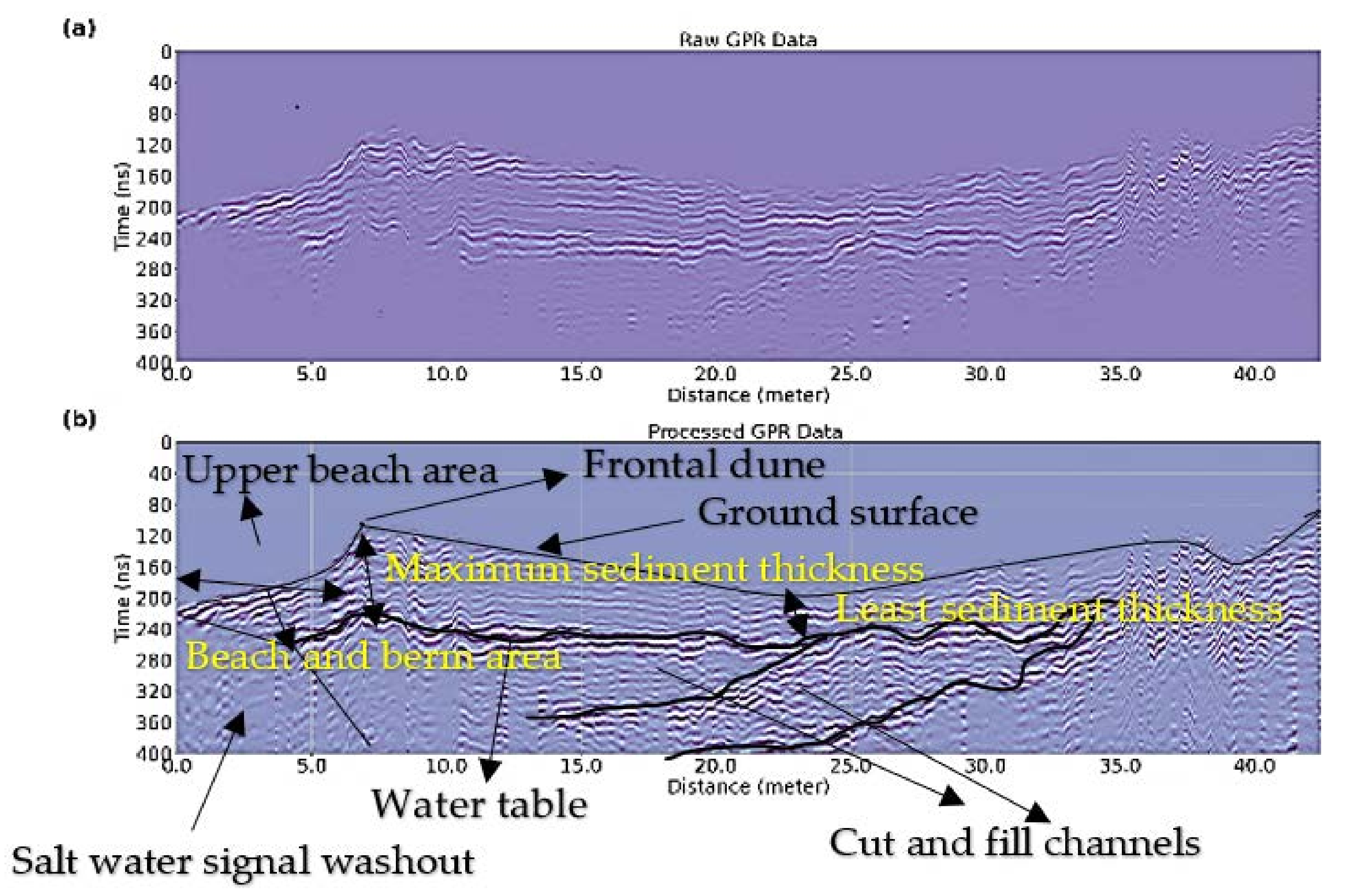
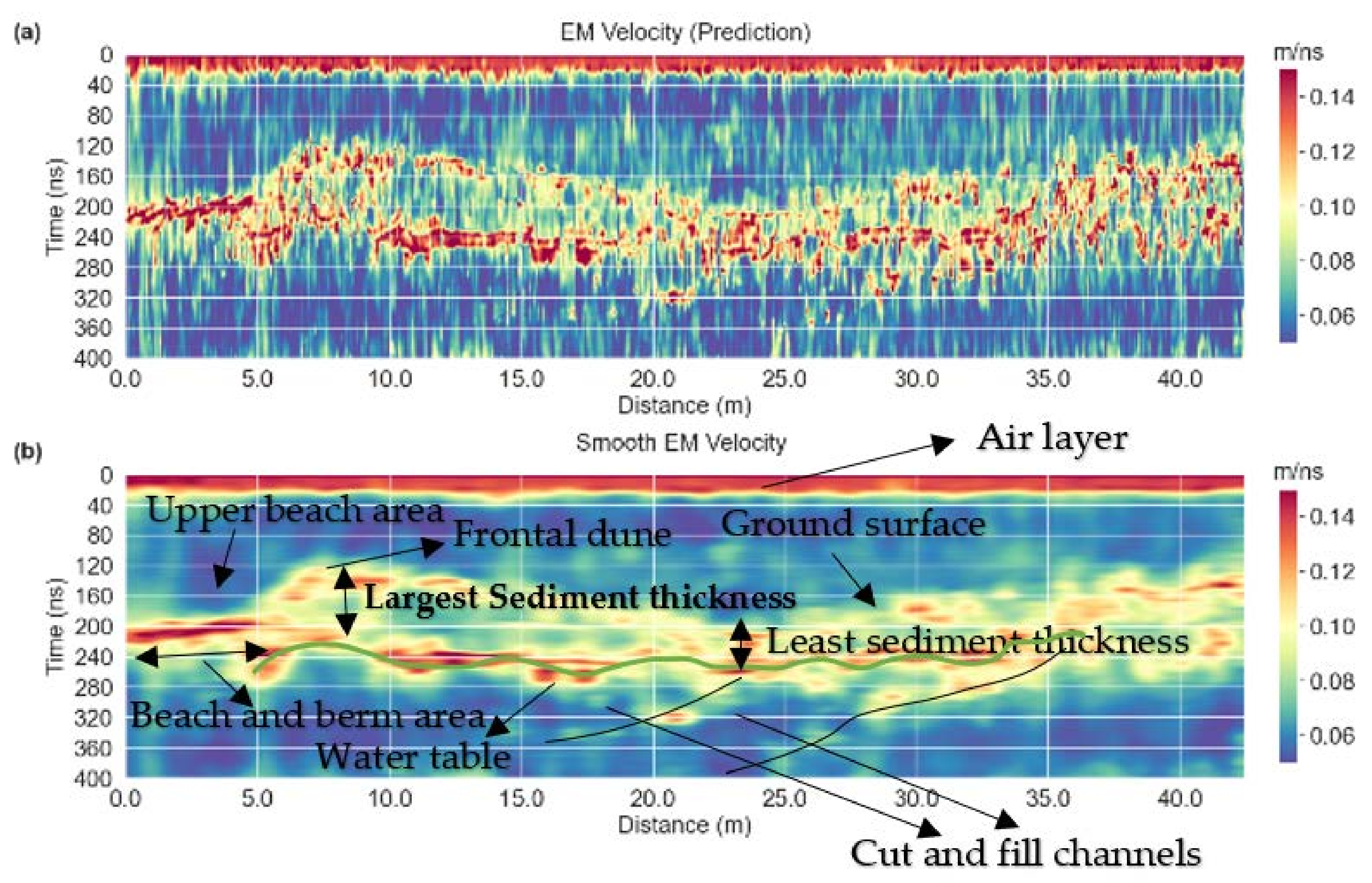
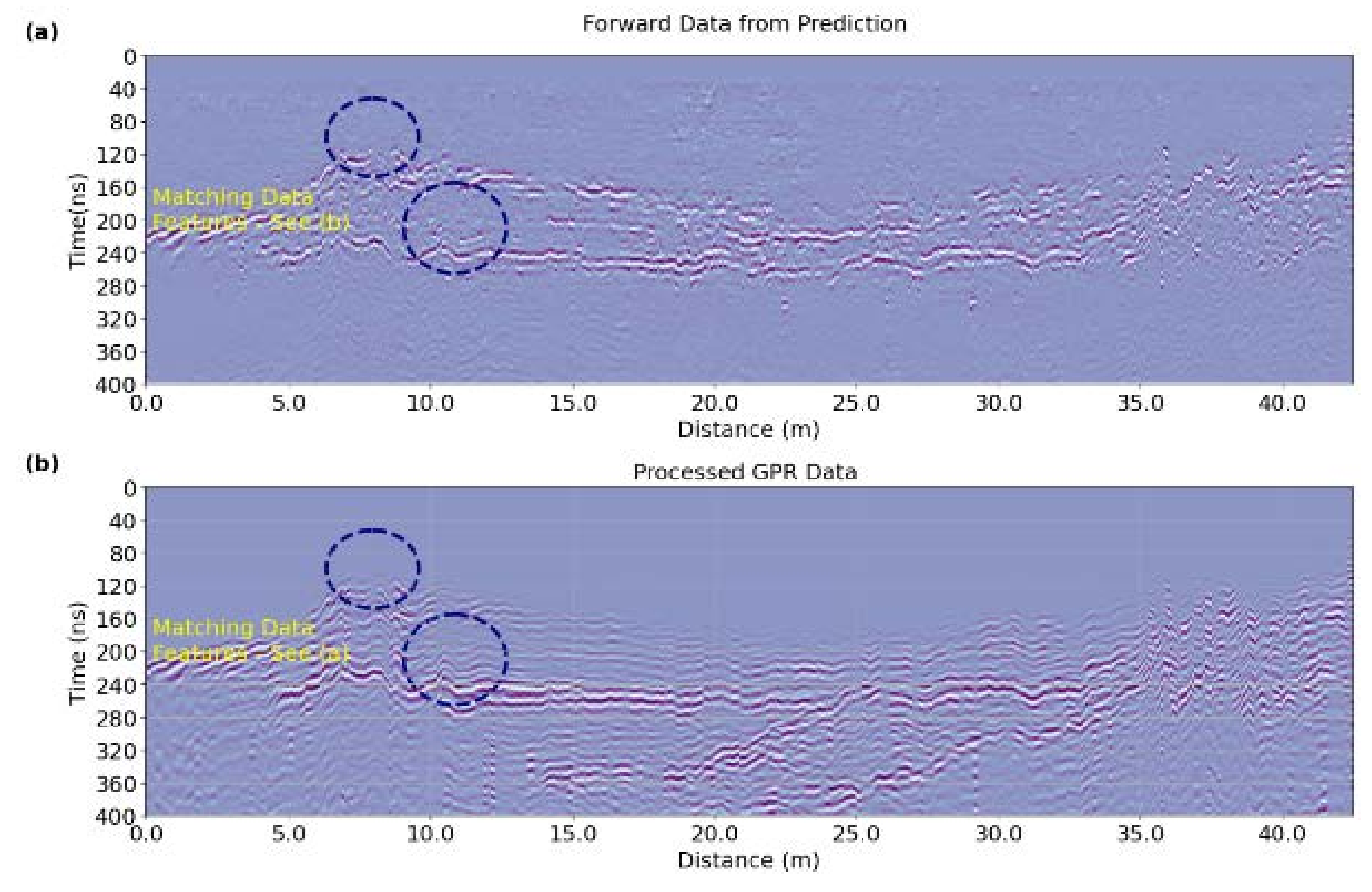
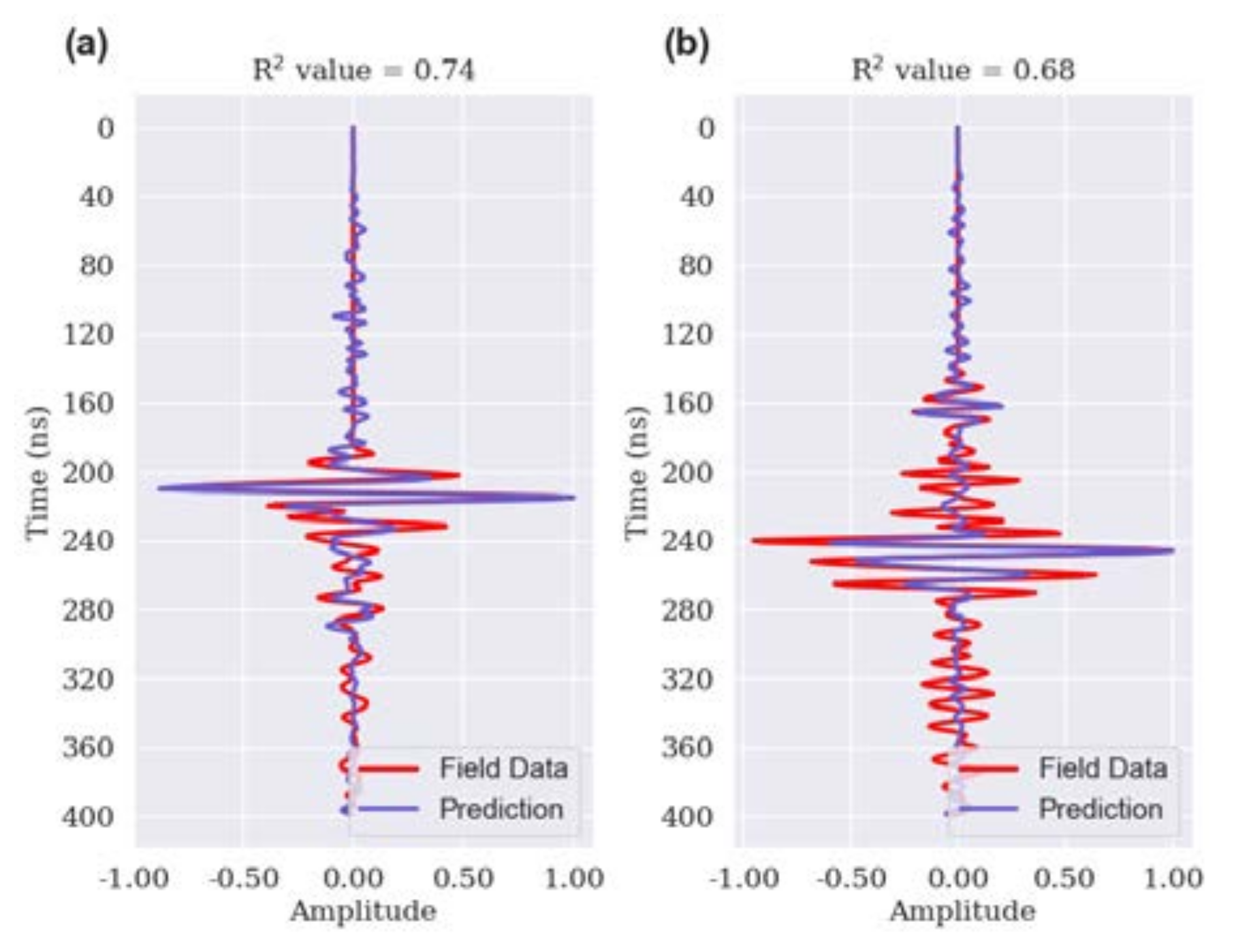
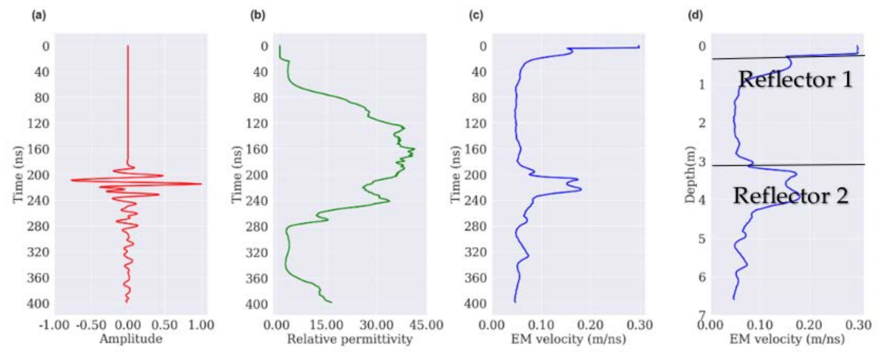
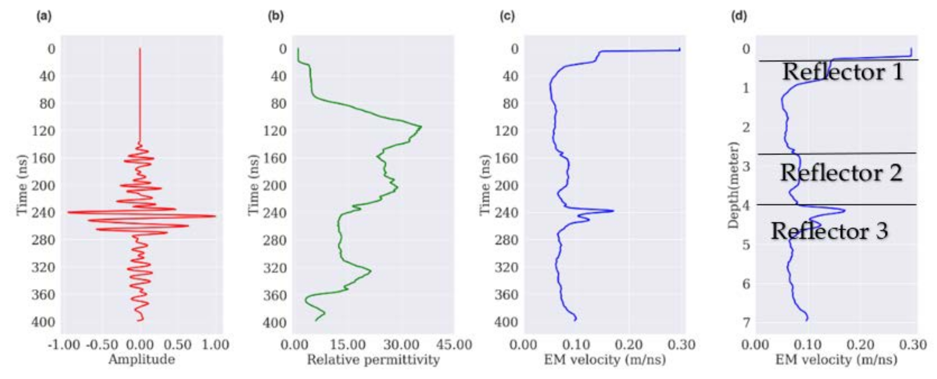
4.3. Application of DCNNs to Field GPR Data

For the application of our DCNNs to field GPR data, another set of synthetic EM velocity models was created with velocity ranging from 0.042 to 0.211 m/ns to capture a wide variety of geological materials. Most common geologic materials have EM velocity values in this range [8]. This velocity range corresponds to ε r   values which start from 2 and go to 50 [8]. Velocity models were also created considering the 4 to 21 layered models. A total of 50,000 velocity models were created. In order to replicate the field scenario, a 2D FDTD scheme with a Ricker source wavelet [36] was used to obtain corresponding GPR traces. As field data contains much noise, the data augmentation process was performed on generated GPR traces to incorporate noise. The steps followed for the data augmentation process were:
(i)
firstly, 50,000 unique datasets were created;
(ii)
secondly, random Gaussian noise was added (approximately 15–85% of the standard deviation of traces amplitude) to unique GPR traces;
(iii)
thirdly, random time gain addition was performed with a range from e3ds to e20ds (where ds is the rate of sampling) to the unique GPR traces;
(iv)
fourthly, random time gain was added to GPR traces having Gaussian noise.
Random time gain was incorporated to account for variation in velocity while travelling in the horizontal direction in the real subsurface. The Ricker wavelet was chosen as the source wavelet during the simulation of synthetic GPR data. As discussed earlier, the Ricker wavelet [36] is useful in GPR signal analysis because the Ricker wavelet provides a good representation of many commercial GPR signals. A total of 1,250,000 datasets were created, with 1.0% (12,500) set aside for validation and 1.0% (12,500) retained for testing. The remaining 98% of datasets were used to train the DCNNs. It took approximately 8 h to complete the training on the high-performance computing facility available at IIT(ISM), Dhanbad, Jharkhand, India. The training process turned out to be very successful, with a validation accuracy (R2) of 0.97119. The field raw GPR data shown in Figure 10a were processed (Figure 10b) before applying them to the trained DCNNs for the prediction of the subsurface EM velocity map.
The processing steps for field GPR data are as follows:
(i)
firstly, the direct waves were removed;
(ii)
secondly, the band-pass filter of frequency range 40–200 MHz was applied;
(iii)
thirdly, time gain addition was carried out;
(iv)
fourthly, max normalization was performed on GPR traces with respect to the maximum amplitude of each GPR trace.
The 40–200 MHz frequency range was chosen for the band-pass filter. There is a practical reason behind choosing this range of frequency. We determined the returned signals frequency using Fast Fourier Transformation (FFT) [40] to justify the chosen cut-offs for the band-pass filter. FFT converts a signal into individual spectral components and thereby provides frequency information concerning the signal. On analyzing many field GPR traces using FFT, we found that frequency from 30 MHz to 50 MHz is dominant in the returned signals, and signals have no frequency distribution in the range of 50 MHz to 200 MHz. Signals have some frequency content after 200 MHz which give information about point features in very shallow subsurface. The significant attenuation in the frequency of signals could be due to the creeping of salt water in the subsurface, which attenuates the EM pulses sent by the GPR transmitter as the locations are just beside the ocean (huge salt content). Additionally, we were concerned about the detection of layered geological features such as sediment thickness, water table, bedrock, location of former channels, etc. and not about point features. In order to detect layered features, we needed to keep the band-pass filter within a low-frequency range. The topographically corrected processed form of GPR data shown in Figure 10b was applied to trained DCNNs for field subsurface EM velocity and relative dielectric permittivity distribution ( ε r ) prediction. Firstly, our DCNNs individually predicted the EM velocity models for all the GPR traces contained in field GPR data. Then, the predicted 1D velocity models were integrated to generate the 2D velocity profile (Figure 11a). To improve the visualization of reflectors in the 2D velocity, they were smoothed down using a Gaussian filter (Figure 11b).
In Figure 11b, one reflector can be seen at the topmost part of the EM velocity map, and two distinct strong reflectors can be seen between 120 ns and 240 ns. The reflector at the top indicates an air layer which was knowingly placed for a set number of nanoseconds in the algorithm to account for the direct arrival of EM pluses from the transmitter to receiver. During the GPR data acquisition on the field, it is usually very difficult to maintain the close contact of the transmitter with the ground surface due to rough terrain, due to which 100% transmission of the generated EM pulses into the ground is not possible. Some EM pulses directly travel through the air and are recorded by the receiver and seen as a reflector in the upper portion of GPR data. The lower reflector, which is between 120 ns and 200 ns, indicates the ground surface. The reflector between 200 ns and 240 ns indicates the water table. The largest and the smallest sediment thickness are also shown in Figure 11b. Between 240 ns and 360 ns, there are former channels such as cut and fill channels, as shown in Figure 11b. All geological features marked in Figure 11b are well correlated with the findings of the previous researchers marked in Figure 8 [25]. Next, forward modeling was performed on the predicted 2D velocity model (Figure 11a) to generate the GPR data using the 2D FDTD method by adopting a zero-offset concept to check the robustness of our DCNNs. The forwarded GPR data shown in Figure 12a show many similar data features which are available in the processed data (Figure 12b). These similar data features are highlighted with circles, which proves the robustness of our DCNNs in forward modeling as well as in inverse modeling. It can also be seen that GPR data after 240 ns in Figure 12a does not match with that of Figure 12b, so it can be said that the prediction of EM velocity shown in Figure 11a after 240 ns is not very reliable. However, up to 240 ns, good matching can be seen regarding GPR data features between Figure 12a (Forwarded GPR data) and Figure 12b (Processed GPR data). Therefore, undoubtedly, it can be said that the smallest and the largest sediment thickness and water table depth were predicted very accurately as all these hydrogeological features lie above and around 240 ns.
In Figure 13, the time domain 2D EM velocity model (Figure 11b) was converted into the depth domain. Comparing the depth of the water table, the smallest and the largest thickness of sediments, and the location of other geological features shown in Figure 13 with the depth and location of the same hydrogeological features shown by researchers [25] in Figure 8, one can say that the prediction of the EM velocity map is quite successful using our DCNNs. The water table can be seen as a strong reflector between 3 m to 4m in depth in Figure 13. It starts approximately from 5 m along the profile length. Normally gradients in groundwater table depth are in the order of 0.001 for a sandy environment [41]. This gradient criterion is also fulfilled by our predicted EM velocity map. In Figure 13, for the profile length of every 5 m, the gradient in water table depth is of order 0.001. The largest and the smallest sediment thickness are approximately 2 m and 1 m above the water table, respectively.
To further check the robustness of our DCNNs in forward and inverse modeling, the selection of two traces was made at different offsets from Figure 12a to compare them with the associated traces in the processed field GPR data shown in Figure 12b, and the matching results are presented in Figure 14a,b. For the GPR traces at 2.53 m and 13.32 m offset, the R 2 values are 0.74 and 0.68, respectively.
Further, the equivalent 1D velocity models in the time and depth domains and relative dielectric permittivity ( ε r ) subsurface distribution plots in the time for trace picked up at 2.53 m (Figure 15a) have been shown in Figure 15b–d.
The equivalent 1D velocity models in the time and depth domains and relative dielectric permittivity ( ε r ) subsurface distribution plots in the time for trace picked up at 13.32 m (Figure 16a) have been shown in Figure 16b–d.
These single 1D velocity models in the time and depth domain, as well as the ε r plot in the time domain at different locations over the study area will help researchers and coastal engineers in their point-based study of the location and aid in determining hydrogeological features such as sediment thickness, water table depth, types of soil, and the depth of the bedrock present in the subsurface in more precise manner needed for the application of coastal erosion mitigation techniques. These 1D velocity models and ε r subsurface distribution plots will also aid in developing coastal sediments compartment boundaries and in identifying landforms. Figure 15a,c show that there is a considerable amount of variation in the GPR trace amplitude values and the EM velocity values between 200 ns and 240 ns, indicating a powerful reflector which is the ground surface (in beach and berm area) at that location. The GPR trace shown in Figure 15a (2.53 m offset) was picked up from the beach and berm area of the beach, which remains mostly saturated with ocean water. Here, ε r varies approximately from 25 to 35 between 200 ns and 240 ns (Figure 15b). These values of ε r correspond to the soil in saturated conditions [8]. As discussed earlier, Reflector 1, shown in Figure 15d, is an air layer that we have added to our algorithm knowingly to account for the direct arrival of EM pulses from the transmitter to the receiver. The ground surface in the beach and berm area is shown as Reflector 2 in Figure 15d. In Figure 16a,c, it can be noticed that there is a considerable variation in amplitude values of the GPR trace and in the EM velocity between 240 ns and 280 ns, which is the ground surface at that location indicated by Reflector 2 in Figure 16d. The ε r values at Reflector 2 vary from 12 to 17 (Figure 16b), indicating that the soil is in a wet condition [8]. The water table shown as Reflector 3 has an approximate depth of 4 m (Figure 16d) at the location where this GPR trace (Figure 16a) was recorded. Reflector 1, again shown in Figure 16d, indicates the air layer. Additionally, two more topographically corrected GPR data profiles were inverted using our DCNNs to obtain a broader picture of the subsurface distribution of EM velocity and ε r over the beach. The results are presented in Figure 17 and Figure 18.
In Figure 17d, one can see two strong reflectors which are very close to each other, between 2 m to 3 m in depth. These two reflectors are very close, making them appear as one reflector and thicker in shape after a profile length of 15 m. The upper reflector is the ground surface, and the lower reflector is the water table at that location. Ground surface, water table, and sediment thickness above the water table are marked out in Figure 17d. In Figure 18d, one can see two distinct reflectors, which are not very strong and are scattered in nature. These two reflectors start at 2 m and remain throughout the profile. These two reflectors are constantly varying in depth. Here, the upper reflector is the ground surface, and the lower reflector is the water table. In between the upper reflector and the lower reflector, sediment thickness is shown.

5. Discussion

In this paper, DeepLabv3+ based newly developed DCNNs were used to predict subsurface EM velocity and ε r subsurface distribution from GPR data to assist in the effective and economical future implementation of coastal erosion mitigation techniques such as beach nourishment over Old Bar Beach, NSW, Australia. Our DCNNs are better than existing DeepLabv3+ based networks such as GPRNet [30] in many ways. Table 1 illustrates our comparative analysis based on seven parameters among GPRNet, DCNNs (having the same values for hyperparameters as GPRNet) and DCNNs having its hyperparameters tuned for decreasing number of trainable parameters and increasing its convergence rate while maintaining good prediction accuracy. The seven parameters selected for comparison are the number of layers, hyperparameters and optimizer, number of trainable parameters, convergence epochs, loss reduction, accuracy in prediction of 1D and 2D EM velocity, and training duration. Table 1 shows that our tuned DCNNs have 16 layers as compared to 23 layers in GPRNet. Additionally, the number of trainable parameters is 1,287,769 in tuned DCNNs compared to 1,392,585 in GPRNet. Although the third column in Table 1, which shows DCNNs having the same values of hyperparameters (filter size, number of filters, filter dilation rate, learning rate) as GPRNet, provides excellent accuracy in 1D and 2D EM velocity prediction, it has high trainable parameters (4,765,961) and a low convergence rate which makes it computationally slow (longer training time) and inefficient in today’s scenario where saving time is important. Our aim was to use a convolutional neural network which has a good prediction accuracy and high convergence rate despite having a lesser number of layers and trainable parameters, and our tuned DCNNs show all these properties. All these factors make our tuned DCNNs computationally fast, efficient, and simple to train and apply to GPR data for EM velocity prediction. The accuracy of EM velocity predictions using tuned DCNNs from 1D synthetic GPR data is high here, as shown in Figure 5. In addition, it was demonstrated that trained weights obtained from the training of tuned DCNNs with 1D datasets can reliably estimate velocities from 2D synthetic GPR data, as shown in Figure 7. After obtaining good results on 2D synthetic GPR data, DCNNs were trained with large 1D synthetic datasets and applied to field GPR data collected from Old Bar Beach for subsurface EM velocity and ε r prediction. Figure 11b reveals how the different hydrogeological features shown as reflectors in the predicted velocity model closely match the hydrogeological features marked by previous researchers in Figure 8 [25]. During prediction, the DCNNs invert GPR traces one by one into 1D velocity models, and a complete 2D velocity model was constructed by combining all inverted 1D velocity models. Our DCNNs-based inversion technique followed in the paper eliminates various earlier assumptions of conventional inversion techniques, including the assumptions of homogeneity and isotropy of each underlying layer. Data augmentation was performed on large synthetic datasets, which were used to train the DCNNs by inserting random Gaussian noise into them to replicate field conditions as field data are usually noisy. Furthermore, temporal gain addition was applied on the synthetic data, compensating for attenuation in EM velocity while traveling in the horizontal direction.
In a real application of the inversion technique in the geophysics domain, the initial guess regarding the initial velocity model of the subsurface, as well as geology knowledge, is crucial for accurate inversion. In DL based inversion, having prior information about the area’s geology makes it easy to choose the EM velocity range for generating synthetic velocity models. This is similar to controlling the unpredictability in velocity generation, so adding previous data (e.g., geological facts) to generate training datasets for velocity assessments for the underlying strata is always a good choice. It can be noticed in Figure 6a that it is an ideal synthetic 2D velocity model. The GPR data obtained in Figure 6b contains only reflections and lack scattering effects and diffractions, which are always present in field data. Seeing the accuracy in 2D velocity prediction shown in Figure 7, it can be said that the GPR data with no scattering effects or diffractions work well in our deep learning method. We can obtain reflections from original GPR data with the help of the diffraction separation technique [42]. Data augmentation in synthetic GPR data revealed that noise and temporal gain addition are required for better results when dealing with field data. Although there is no thumb rule to decide how many datasets should be used to train the DCNNs to obtain reliable EM velocity findings, in our study, it can be said that the number of datasets used for training is good enough as we obtained reliable predicted EM velocity distributions over the study area as well as accurate depth and locations of different hydrogeological features such as the maximum and the minimum thickness of sediment, water table depth, locations of former channels, and salt water intrusion zone. These findings will be very much useful for the future implementation of coastal erosion mitigating techniques. All results successfully show that our DeepLabv3+ based DCNNs along with GPR can be conveniently and successfully used in coastal environments for the quick and accurate hydrogeological investigation required for the application of coastal erosion mitigation methods such as beach nourishment in Australia and around the world.

6. Conclusions

In this paper, DeepLabv3+ based deep convolutional neural networks (DCNNs) shown in Figure 3 were initially trained and validated on small synthetic datasets containing 9900 1D GPR traces and corresponding EM velocity models. The DCNNs turned out to be quite promising, with training, validation, and testing accuracy of approximately 95%, 94%, and 95%, respectively (Figure 4b,d and Figure 5). Then, 1D trained model weights were applied to 2D synthetic GPR data for EM velocity prediction and the accuracy of prediction was approximately 95% (Figure 7). Based on results obtained from 1D and 2D synthetic GPR data, it can be said that our DCNNs have a well-designed encoder–decoder system and does an excellent job in predicting EM velocity models. Seeing the excellent performance of DCNNs in 2D EM velocity prediction using 1D trained model weights, a large number of 1D synthetic datasets (approximately 1.2 million) were generated and Gaussian noise was added to them to replicate the real field scenario to train the DCNNs. The DCNNs trained with the large 1D synthetic datasets were applied to three sets of field GPR data acquired at different locations on Old Bar Beach, NSW, Australia, to obtain the subsurface EM velocity map and relative dielectric permittivity ( ε r ) distribution plots (Figure 11, Figure 13, Figure 15b, Figure 16b, Figure 17b,d and Figure 18b,d) to identify the hydrogeological features such as the smallest and the largest sediment thickness, depth of water table, locations of former channels, types of soil, and other subsurface structural features which will help researchers and coastal engineers in the future to effectively implement coastal erosion mitigating techniques such as beach nourishment over eroding coastal areas. Comparing the results presented in this paper with the findings of previous studies carried out in the Old Bar Beach region using GPR (Figure 8), it can be said that our DCNNs with a lesser number of trainable parameters, a lesser number of layers, and a high convergence rate can perform GPR data inversion commendably well in coastal environments.

Author Contributions

Conceptualization, A.K., U.K.S. and B.P.; methodology, A.K.; code, A.K.; validation, A.K., U.K.S. and B.P.; formal analysis, A.K.; investigation, A.K., U.K.S. and B.P.; data curation, A.K. and U.K.S.; writing—original draft preparation, A.K.; writing—review and editing, A.K., U.K.S. and B.P.; visualization, A.K., U.K.S. and B.P.; supervision, U.K.S. and B.P. All authors have read and agreed to the published version of the manuscript.

Funding

This study was supported by the Centre for Advanced Modelling and Geospatial Information Systems (CAMGIS), Faculty of Engineering and IT, University of Technology Sydney with grant number 232487.

Institutional Review Board Statement

Not applicable.

Informed Consent Statement

Not applicable.

Data Availability Statement

Publicly available datasets were analyzed in this study. This data can be found here: http://pid.geoscience.gov.au/dataset/ga/100224.

Acknowledgments

The authors would like to express their gratitude to the IIT(ISM), Dhanbad, India, for providing a pleasant environment to pursue these studies. The authors would also like to extend special thanks to Geoscience Australia, which is Australia’s pre-eminent public sector geoscience organization, for making GPR data and models accessible to the public. The Science and Engineering Research Board, Department of Science and Technology, New Delhi, India, provided technical support to the authors, which is gratefully acknowledged. We wish to thank the editors for handling the manuscript and the reviewers for their helpful and constructive comments and suggestions, which have significantly improved the manuscript.

Conflicts of Interest

The authors declare no conflict of interest.

References

  1. Kinsela, M.A.; Hanslow, D.J. Coastal erosion risk assessment in New South Wales: Limitations and potential future directions. In Proceedings of the 22nd NSW Coastal Conference 2013, Port Macquarie, NSW, Australia, 12–15 November 2013. [Google Scholar] [CrossRef]
  2. Liew, M.; Xiao, M.; Jones, B.M.; Farquharson, L.M.; Romanovsky, V.E. Prevention and control measures for coastal erosion in northern high-latitude communities: A systematic review based on Alaskan case studies. Environ. Res. Lett. 2020, 15, 093002. [Google Scholar] [CrossRef]
  3. Staudt, F.; Gijsman, R.; Ganal, C.; Mielck, F.; Wolbring, J.; Hass, H.C.; Goseberg, N.; Schüttrumpf, H.; Schlurmann, T.; Schimmels, S. The sustainability of beach nourishments: A review of nourishment and environmental monitoring practice. J. Coast. Conserv. 2021, 25, 34. [Google Scholar] [CrossRef]
  4. Switzer, A.D.; Gouramanis, C.; Bristow, C.S.; Simms, A.R. Ground-penetrating radar (GPR) in coastal hazard studies. In Geological Records of Tsunamis and other Extreme Waves; Elsevier: Amsterdam, The Netherlands, 2020; pp. 143–168. [Google Scholar] [CrossRef]
  5. Singh, K.K.; Kulkarni, A.V.; Mishra, V.D. Estimation of glacier depth and moraine cover study using ground penetrating radar (GPR) in the Himalayan region. J. Indian Soc. Remote Sens. 2010, 38, 1–9. [Google Scholar] [CrossRef]
  6. Piro, S.; Campana, S. GPR investigation in different archaeological sites in Tuscany (Italy). Analysis and comparison of the obtained results. Near Surf. Geophys. 2012, 10, 47–56. [Google Scholar] [CrossRef]
  7. Liu, L.; Xie, X. GPR for geotechnical engineering. J. Geophys. Eng. 2013, 10, 030201. [Google Scholar] [CrossRef]
  8. Baker, G.S.; Jordan, T.E.; Pardy, J. An introduction to ground penetrating radar (GPR). Spec. Pap. Geol. Soc. Am. 2007, 432, 1. [Google Scholar] [CrossRef]
  9. Virieux, J.; Operto, S. An overview of full-waveform inversion in exploration geophysics. Geophysics 2009, 74, WCC1–WCC26. [Google Scholar] [CrossRef]
  10. Kim, Y.; Nakata, N. Geophysical inversion versus machine learning in inverse problems. Lead. Edge 2018, 37, 894–901. [Google Scholar] [CrossRef]
  11. Smirnov, E.A.; Timoshenko, D.M.; Andrianov, S.N. Comparison of regularization methods for imagenet classification with deep convolutional neural networks. Aasri Procedia 2014, 6, 89–94. [Google Scholar] [CrossRef]
  12. Xiong, Y.; Zuo, R.; Carranza, E.J.M. Mapping mineral prospectivity through big data analytics and a deep learning algorithm. Ore Geol. Rev. 2018, 102, 811–817. [Google Scholar] [CrossRef]
  13. Waldeland, A.U.; Jensen, A.C.; Gelius, L.J.; Solberg, A.H.S. Convolutional neural networks for automated seismic interpretation. Lead. Edge 2018, 37, 529–537. [Google Scholar] [CrossRef]
  14. Araya-Polo, M.; Dahlke, T.; Frogner, C.; Zhang, C.; Poggio, T.; Hohl, D. Automated fault detection without seismic processing. Lead. Edge 2017, 36, 208–214. [Google Scholar] [CrossRef]
  15. Li, S.; Liu, B.; Ren, Y.; Chen, Y.; Yang, S.; Wang, Y.; Jiang, P. Deep-learning inversion of seismic data. IEEE Trans. Geosci. Remote Sens. 2020, 58, 2135–2149. [Google Scholar] [CrossRef]
  16. Wu, Y.; Lin, Y. InversionNet: An efficient and accurate data-driven full waveform inversion. IEEE Trans. Comput. Imaging 2019, 6, 419–433. [Google Scholar] [CrossRef]
  17. Yang, F.; Ma, J. Deep−learning inversion: A next-generation seismic velocity model building method. Geophysics 2019, 84, R583–R599. [Google Scholar] [CrossRef]
  18. Bralich, J.; Reichman, D.; Collins, L.M.; Malof, J.M. Improving convolutional neural networks for buried target detection in ground penetrating radar using transfer learning via pretraining. In Detection and Sensing of Mines, Explosive Objects, and Obscured Targets XXII; SPIE: Bellingham, WA, USA, 2017; Volume 10182, pp. 198–208. [Google Scholar] [CrossRef]
  19. Yue, Y.; Liu, H.; Meng, X.; Li, Y.; Du, Y. Generation of High-Precision Ground Penetrating Radar Images Using Improved Least Square Generative Adversarial Networks. Remote Sens. 2021, 13, 4590. [Google Scholar] [CrossRef]
  20. Chen, W.; Pourghasemi, H.R.; Kornejady, A.; Zhang, N. Landslide spatial modeling: Introducing new ensembles of ANN, MaxEnt, and SVM machine learning techniques. Geoderma 2017, 305, 314–327. [Google Scholar] [CrossRef]
  21. Elmahdy, S.; Ali, T.; Mohamed, M. Flash Flood Susceptibility modeling and magnitude index using machine learning and geohydrological models: A modified hybrid approach. Remote Sens. 2020, 12, 2695. [Google Scholar] [CrossRef]
  22. Mohajane, M.; Costache, R.; Karimi, F.; Pham, Q.B.; Essahlaoui, A.; Nguyen, H.; Laneve, G.; Oudija, F. Application of remote sensing and machine learning algorithms for forest fire mapping in a Mediterranean area. Ecol. Indic. 2021, 129, 107869. [Google Scholar] [CrossRef]
  23. Chen, L.C.; Zhu, Y.; Papandreou, G.; Schroff, F.; Adam, H. Encoder-decoder with atrous separable convolution for semantic image segmentation. In Proceedings of the European Conference on Computer Vision (ECCV), Munich, Germany, 8–14 September 2018; pp. 801–818. [Google Scholar] [CrossRef]
  24. Chen, L.-C.; Papandreou, G.; Schroff, F.; Adam, H. Rethinking atrous convolution for semantic image segmentation. arXiv 2017, arXiv:1706.05587. [Google Scholar]
  25. Howard, F.J.F. Ground Penetrating Radar (GPR) Data—Old Bar Beach Survey; Geoscience: Canberra, Australia, 2016. [Google Scholar]
  26. Irving, J.; Knight, R. Numerical modeling of ground-penetrating radar in 2-D using MATLAB. Comput. Geosci. 2006, 32, 1247–1258. [Google Scholar] [CrossRef]
  27. Kuzuoglu, M.; Mittra, R. Frequency dependence of the constitutive parameters of causal perfectly matched anisotropic absorbers. IEEE Microw. Guided Wave Lett. 1996, 6, 447–449. [Google Scholar] [CrossRef]
  28. Chen, Y.H.; Chew, W.C.; Oristaglio, M.L. Application of perfectly matched layers to the transient modeling of subsurface EM problems. Geophysics 1997, 62, 1730–1736. [Google Scholar] [CrossRef]
  29. Kitsunezaki, N. Electro-magnetic Simulation Based on the Integral Form of Maxwell’s Equations. In Recent Advances in Integral Equations; Intech Open: London, UK, 2018; p. 63. [Google Scholar] [CrossRef]
  30. Leong, Z.X.; Zhu, T. Direct velocity inversion of ground penetrating radar data using GPRNet. J. Geophys. Res. Solid Earth 2021, 126, e2020JB021047. [Google Scholar] [CrossRef]
  31. Nair, V.; Hinton, G.E. Rectified linear units improve restricted Boltzmann machines. In Proceedings of the 27th International Conference on Machine Learning, Haifa, Israel, 21–24 June 2010; pp. 807–814. [Google Scholar]
  32. Kingma, D.P.; Ba, J. Adam: A method for stochastic optimization. arXiv 2014, arXiv:1412.6980. [Google Scholar] [CrossRef]
  33. Sara, U.; Akter, M.; Uddin, M.S. Image quality assessment through FSIM, SSIM, MSE and PSNR—A comparative study. J. Comput. Commun. 2019, 7, 8–18. [Google Scholar] [CrossRef] [Green Version]
  34. Neal, A. Ground-penetrating radar and its use in sedimentology: Principles, problems and progress. Earth-Sci. Rev. 2004, 66, 261–330. [Google Scholar] [CrossRef]
  35. Gholamy, A.; Kreinovich, V. Why Ricker wavelets are successful in processing seismic data: Towards a theoretical explanation. In Proceedings of the 2014 IEEE Symposium on Computational Intelligence for Engineering Solutions (CIES), Orlando, FL, USA, 9–12 December 2014; IEEE: Piscataway, NJ, USA, 2014; pp. 11–16. [Google Scholar] [CrossRef]
  36. Bradford, J.H.; Wu, Y. Instantaneous spectral analysis: Time-frequency mapping via wavelet matching with application to contaminated-site characterization by 3D GPR. Lead. Edge 2007, 26, 1018–1023. [Google Scholar] [CrossRef]
  37. Kumar, V.; Maiti, S. A nobel characterization of shape of pulse in GPR signal transmission. In Proceedings of the 2014 International Conference on Communication and Signal Processing, Melmaruvathur, India, 3–5 April 2014; pp. 944–947. [Google Scholar] [CrossRef]
  38. Rosen, P.S. Water table. In Beaches and Coastal Geology. Encyclopedia of Earth Sciences Series; Springer: New York, NY, USA, 1982. [Google Scholar] [CrossRef]
  39. McPherson, A.; Hazelwood, M.; Moore, D.; Owen, K.; Nichol, S.; Howard, F. The Australian Coastal Sediment Compartments Project: Methodology and Product Development. Record 2015/25; Geoscience: Canberra, Australia, 2015. [Google Scholar] [CrossRef]
  40. Harčarik, T.; Bocko, J.; Masláková, K. Frequency analysis of acoustic signal using the Fast Fourier Transformation in MATLAB. Procedia Eng. 2012, 48, 199–204. [Google Scholar] [CrossRef]
  41. Timms, W.; Acworth, R.I.; Berhane, D. Shallow groundwater dynamics in smectite dominated clay on the Liverpool Plains of New South Wales. Soil Res. 2001, 39, 203–218. [Google Scholar] [CrossRef]
  42. Merzlikin, D.; Fomel, S.; Sen, M.K. Least-squares path summation diffraction imaging using sparsity constraints. Geophysics 2019, 84, S187–S200. [Google Scholar] [CrossRef]
Figure 1. The “Yee lattice” [29] is used to discretize equations of Maxwell in space. The orientation of components of the electric (E) and magnetic field (H) in the x, y, and z directions can be seen here. Here, i, j, and k denote the values of the co-ordinates in the x, y, and z directions, respectively.
Remotesensing 14 04899 g001
Figure 2. The orientation of transmitter (Tx) and receiver (Rx) in the TM polarization mode of GPR data acquisition [8].
Remotesensing 14 04899 g002
Figure 3. Schematic diagram of DeepLabv3+ based our Deep Convolutional Neural Networks (DCNNs).
Remotesensing 14 04899 g003
Figure 4. (a) Loss versus epochs plot for training, (b) R2 versus epochs plot for training, (c) loss versus epochs for validation, and (d) R2 versus epochs for validation.
Remotesensing 14 04899 g004
Figure 5. (ac) show matching results of three randomly selected 1D true velocity models with corresponding predicted velocity models.
Remotesensing 14 04899 g005
Figure 6. (a) The simple 2D synthetic EM velocity profile, (b) the simulated 2D synthetic GPR data, and (c) the predicted EM velocity.
Remotesensing 14 04899 g006
Figure 7. (ac) show the matching results of three selected velocity models at different offsets (Figure 6a) with corresponding DCNNs based inverted velocity models (Figure 6c).
Remotesensing 14 04899 g007
Figure 8. The topographically corrected processed form of field GPR data collected from the Old Bar Beach, New South Wales, Australia, by previous researchers [25]. Different hydrogeological features have been marked on it by them.
Remotesensing 14 04899 g008
Figure 9. Coastal sediment compartment boundaries in MAP 2 and landform types in MAP 1 from Old Bar Beach, NSW, Australia. A GPR survey was carried out along 18 profiles (P) denoted by small saffron lines in MAP 1, which are perpendicular to the surface water line except for P11. Profiles (P) denoted by P6, P8, and P12 in green circles in MAP 1 were studied in our research. All GPR data were acquired within a geographical bounding box shown with a yellow rectangular box in MAP 2 with coordinates 152.54°, −32.35°, 152.60°, and −31.97° for west longitude, south latitude, east longitude, and north latitude, respectively [25].
Remotesensing 14 04899 g009
Figure 10. (a) The raw field GPR data, and (b) the processed GPR data. Both raw and processed GPR data are topographically corrected. On comparing Figure 10b with Figure 8, one could see the water table at around 240 ns in Figure 10b and other features such as cut and fill channels are between 240 ns and 400 ns.
Remotesensing 14 04899 g010
Figure 11. (a) The DCNNs based inverted 2D EM velocity model. (b) The smoothed 2D EM velocity model obtained using Gaussian filter.
Remotesensing 14 04899 g011
Figure 12. (a) The GPR data obtained by performing forward modeling on predicted EM velocity, as shown in Figure 11a. (b) Processed field GPR data.
Remotesensing 14 04899 g012
Figure 13. The subsurface EM velocity map in the depth domain for Old Bar Beach, NSW, Australia.
Remotesensing 14 04899 g013
Figure 14. (a) The matching result for GPR traces picked up from Figure 12a,b at 2.53 m offset. (b) The matching result for GPR traces picked up from Figure 12a,b at 13.32 m offset.
Remotesensing 14 04899 g014
Figure 15. (a) GPR trace at 2.53 m offset in the time domain, (b) the variation of ε r in the time domain, (c) EM velocity in the time domain, and (d) EM velocity in the depth domain.
Remotesensing 14 04899 g015
Figure 16. (a) GPR trace at 13.32m offset in time depth domain, (b) the variation of ε r in the time domain, (c) EM velocity in the time domain, and (d) EM velocity in the depth domain.
Remotesensing 14 04899 g016
Figure 17. (a) Topographically corrected raw GPR data, (b) predicted velocity map in the time domain, (c) processed GPR data, and (d) velocity map in the depth domain.
Remotesensing 14 04899 g017
Figure 18. (a) Topographically corrected raw GPR data, (b) predicted velocity map in the time domain, (c) processed GPR data, and (d) velocity map in the depth domain.
Remotesensing 14 04899 g018
Table 1. Comparison between existing DeepLabv3+ based networks (GPRNet) and our two versions of DCNNs. The parameters considered for comparison are the number of layers, hyperparameters and optimizer, number of trainable parameters, convergence epochs, loss reduction, accuracy, and training duration.
ParametersDeepLabv3+ Based GPRNetDeepLabv3+ Based DCNNs
(Having Same Values for Hyperparameters as GPRNet Has)
DeepLabv3+ Based Tuned DCNNs(Hyperparameters Tuned to Reduce Number of Trainable Parameters and Increase Convergence Rate)
Number of layers23 layers16 layers16 layers
Encoder (14 layers)Decoder (9 layers)Encoder (8 layers)Decoder (8 layersEncoder (8 layers)Decoder (8 layers)
4 Convolutions +
4 Pooling + 4 Dilated Convolutions + 1 Merged Convolution + 1 Merged Up-sampling
5 Deconvolutions + 4 Up-sampling4 Convolutions +
4 Pooling
1 Deconvolutions + 3 Dilated Deconvolutions + 4 Up-sampling4 Convolutions +
4 Pooling
1 Deconvolutions + 3 Dilated Deconvolutions + 4 Up-sampling
Hyperparameters and optimizerFilter size = 20, Initial number of filters = 16, Learning rate = 0.0001, Filter size dilation rate = 6, 12, 18, Optimizer = AdamFilter size = 20, Initial number of filters = 16, Learning rate = 0.0001, Filter size dilation rate = 6, 12, 18, Optimizer = AdamFilter size = 12, Initial number of filters = 12, Learning rate = 0.0001, Filter size dilation rate = 3, 6, 9, Optimizer = Adam
Number of trainable parameters1,392,5854,765,9611,287,769
Convergence epochs (Iterations)10015171
Loss reduction (MSE)0.00008750.0000750.000095
Accuracy (R2)1D Case2D Case1D Case2D Case1D Case2D Case
99%98%99%99%99%95%
Training duration3 h4.5 h1.5 h
Publisher’s Note: MDPI stays neutral with regard to jurisdictional claims in published maps and institutional affiliations.

