Article

Monitoring Non-Linear Ground Motion above Underground Gas Storage Using GNSS and PSInSAR Based on Sentinel-1 Data

1
Department of Geoinformatics, Faculty of Mining and Geology, VŠB–Technical University of Ostrava, 17. Listopadu 2172/15, 708 00 Ostrava–Poruba, Czech Republic
2
IT4Innovations National Supercomputing Center, VŠB–Technical University of Ostrava, 17. Listopadu 2172/15, 708 00 Ostrava–Poruba, Czech Republic
*
Author to whom correspondence should be addressed.
Remote Sens. 2022, 14(19), 4898; https://doi.org/10.3390/rs14194898
Submission received: 14 July 2022 / Revised: 19 September 2022 / Accepted: 27 September 2022 / Published: 30 September 2022

Abstract

:
Several methods allow accurate measurement of terrain surface motions. Global navigation satellite systems (GNSSes) and interferometry with synthetic aperture radar (InSAR) stand out in terms of measurement accuracy among them. In principle, both methods make it possible to evaluate a three-dimensional vector of the motion of points on the terrain surface. In this work, we dealt with the evaluation of motions in the up–down (U–D) and east–west direction (E–W) over underground gas storage (UGS) from InSAR. One crucial step in breaking down PSInSAR line of sight (LOS) measurements to U–D and E–W components is getting time series derived from individual tracks to the same time frame. This is usually performed by interpolation, but we used an innovative approach: we analyzed individual time series using the Lomb–Scargle periodogram (LSP), which is suitable for periodic noisy and irregularly sampled data; we selected the most significant period, created LSP models, and used them instead of the original time series. Then, it was possible to derive time series values for any arbitrary time step. To validate the results, we installed one GNSS receiver in the Tvrdonice UGS test area to perform independent measurements. The results show a good agreement in the evaluation of motions by both methods. The correlation coefficient between horizontal components from both PSInSAR and GNSS was 0.95 in the case of the E–W component, with an RMSE of 1.75 mm; for U–D they were 0.78 and 2.35 mm, respectively. In addition to comparing the motions in the U–D and E–W directions, we also created a comparison by converting GNSS measurements to a line of sight of the Sentinel-1 satellite to evaluate the conformity of InSAR and GNSS measurements. Based on descending track, the correlation coefficient between LOS from both methods is, on average, 0.97, with an RMSE of 2.70 mm.

1. Introduction

Radar interferometry is a widely used technique of aerial monitoring of slow motions on the Earth’s surface. It can provide valuable information on the behavior of an underground geological structure, whether it is used as a source of water, oil, or gas, a CO2 storage space, or, for example, as an underground gas storage facility (UGS). The periodic motions of the Earth’s surface enable, among other things, detection of unused parts of the reservoir, reactivation of faults, or failure of wells, and can be used for tuning, verification, and validation of geotechnical models of underground geological structures in which UGS facilities are built [1,2,3,4,5]. The great advantage of this method is the aerial coverage, the detail of the description in space, high sensitivity, and the ability to monitor the development of terrain surface shifts over time. The disadvantage is the small detail in the time dimension because repeated data collection is performed in a period from days to weeks. A lack of well-reflecting surfaces that can function as permanent scatterers (PSes) can be a limitation.
The advantage of global navigation satellite system (GNSS) technology is that it is an independent, very accurate method, allowing detailed data to be collected over time [2,6,7]. Its disadvantage is its ability to cover the studied area only with a sparse network of points due to the high costs associated with the installation and long-term operation of GNSS reference stations [8,9]. For example, [1] used a network of 39 GPS (global positioning system) receivers for benchmarking. He compared the average time series of deformations from PS points in a radius of 100 m around the GPS receiver with the measurements from this receiver. Both measurements were evaluated relative to the selected reference point. In the case of InSAR, using a reference point is directly part of the method; in the case of GPS measurements, selecting one of the 39 receivers as a reference point was necessary. The horizontal displacement rates measured by InSAR agreed with GPS measurements within 1.8 mm a year, and the vertical displacement rates agreed within 4.8 mm a year [1]. A worse result in the vertical direction may be explained by the general lower quality of GNSS in determining the vertical component than in the case of the horizontal components. In contrast, in the case of InSAR, higher accuracy can be expected in the vertical direction [10].
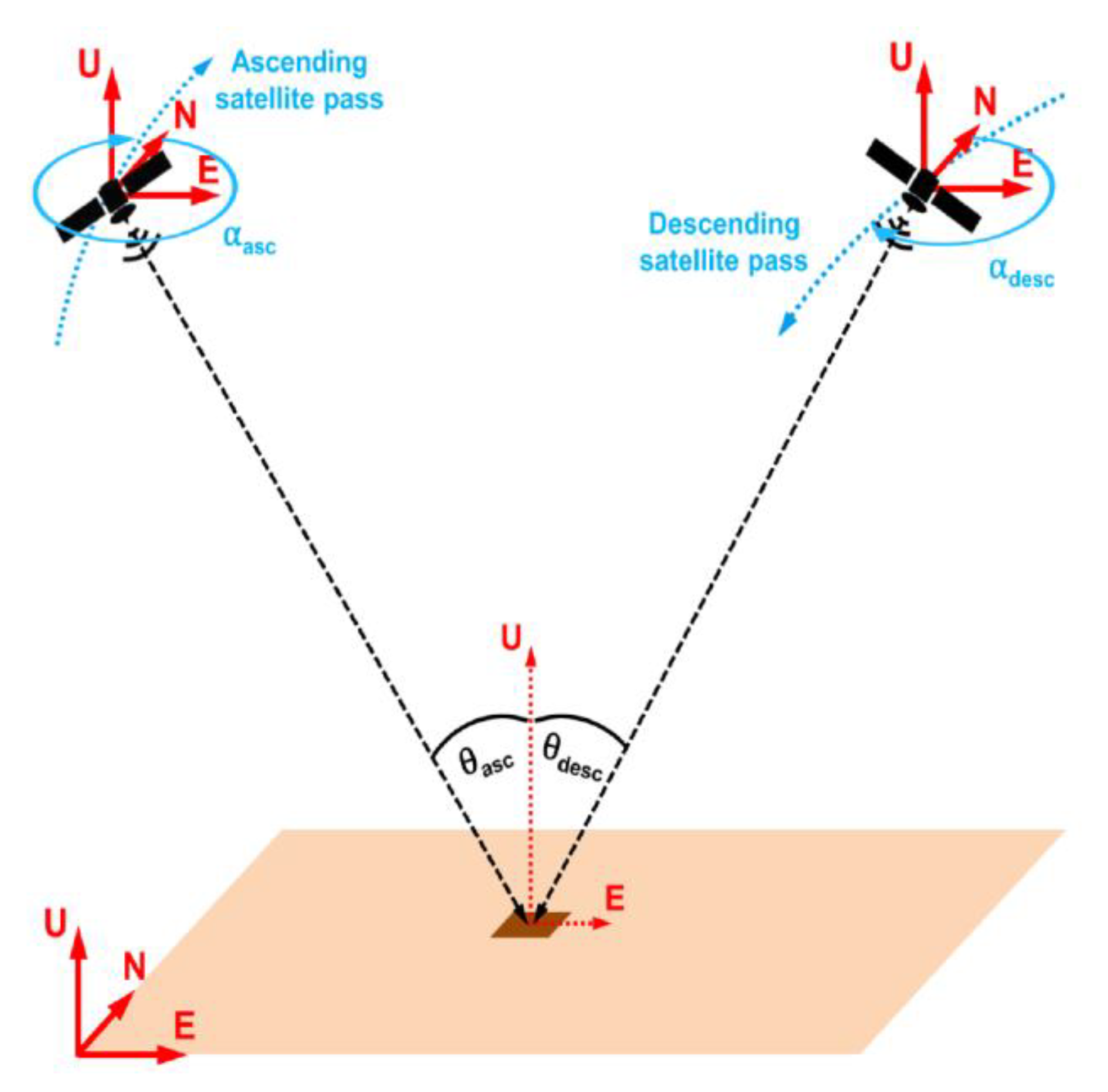
In radar interferometry, the change in distance between the satellite and the monitored point on the surface is evaluated, i.e., the change in their distance in line of sight (LOS), which is one-dimensional [1]. However, the motion of the terrain surface, caused for example by underground processes, is three-dimensional. The one-dimensional nature of LOS implies that it is not easy to obtain a complete 3D description of terrain motion. For this reason, the direct use of LOS for vertical motion can lead to misinterpretation of the results. In addition, a simple conversion of LOS to vertical motion by cosine transformation, which completely neglects the horizontal component of motion, can lead to erroneous conclusions [5,11].
However, concerning measurement geometry and orbiting satellite motion, measured displacements in LOS can be broken down into three directions by combined processing of data obtained on both ascending and descending satellite tracks [2,11,12]. Given the orbits of the satellites, which are usually sub-polar, the method is relatively sensitive to horizontal motions in the east–west (E–W) direction but is almost insensitive to the motions in the north–south (N–S) direction (except for polar areas). Therefore, it is not possible to evaluate the complete horizontal motion vector of the monitored point from the measurement. However, even the E–W component itself can, in some situations, provide interesting information about the behavior of the area over time. For example, this method can describe, in more detail, the deformation of the east or west-facing slopes in the E–W direction. The same applies to areas above underground gas storage. They are usually flat, and the E–W component could provide at least partial information about the behavior of the overburden of the UGS’s geological structure during the natural gas injection/withdrawal cycle. The same applies for geological faults that intersect the monitored area.
The problem of motion vector breakdown from the LOS direction into its components is not new; it was first addressed by Hoffmann and Zebker [13] and especially by Wright et al. [14], and then, for example, by [1,2,11,15].
Among other things, the evaluation of 3D terrain displacements is used for tuning, verifying, and validating the geomechanical model of the studied geological structure [1,10]. However, recently the inverse approach has emerged—the use of a deformation model based on knowledge of the change in the volume of underground fluids, based on Green’s function, which allows the use of a single-track LOS to derive a 3D vector of motion of the terrain ([16] in [17]). However, the necessary condition is the existence of a geomechanical model of the storage structure.
Some papers have also compared the E–W component of displacement obtained from PSInSAR with GNSS measurements. They were typically focused on monitoring motions of the area affected by subsidence, e.g., due to excessive groundwater withdrawal [18], hydrocarbon production [1], or underground coal mining [2,11]. Studies can also be found that deal with comparing landslides measurement results using GNSS and InSAR or the integration of measurement results obtained by both methods [8,19,20,21,22]. However, only a few papers so far have dealt with long-term monitoring of the cyclical horizontal motion of the terrain above an underground gas storage and its relation to the area’s geology, e.g., [23,24].
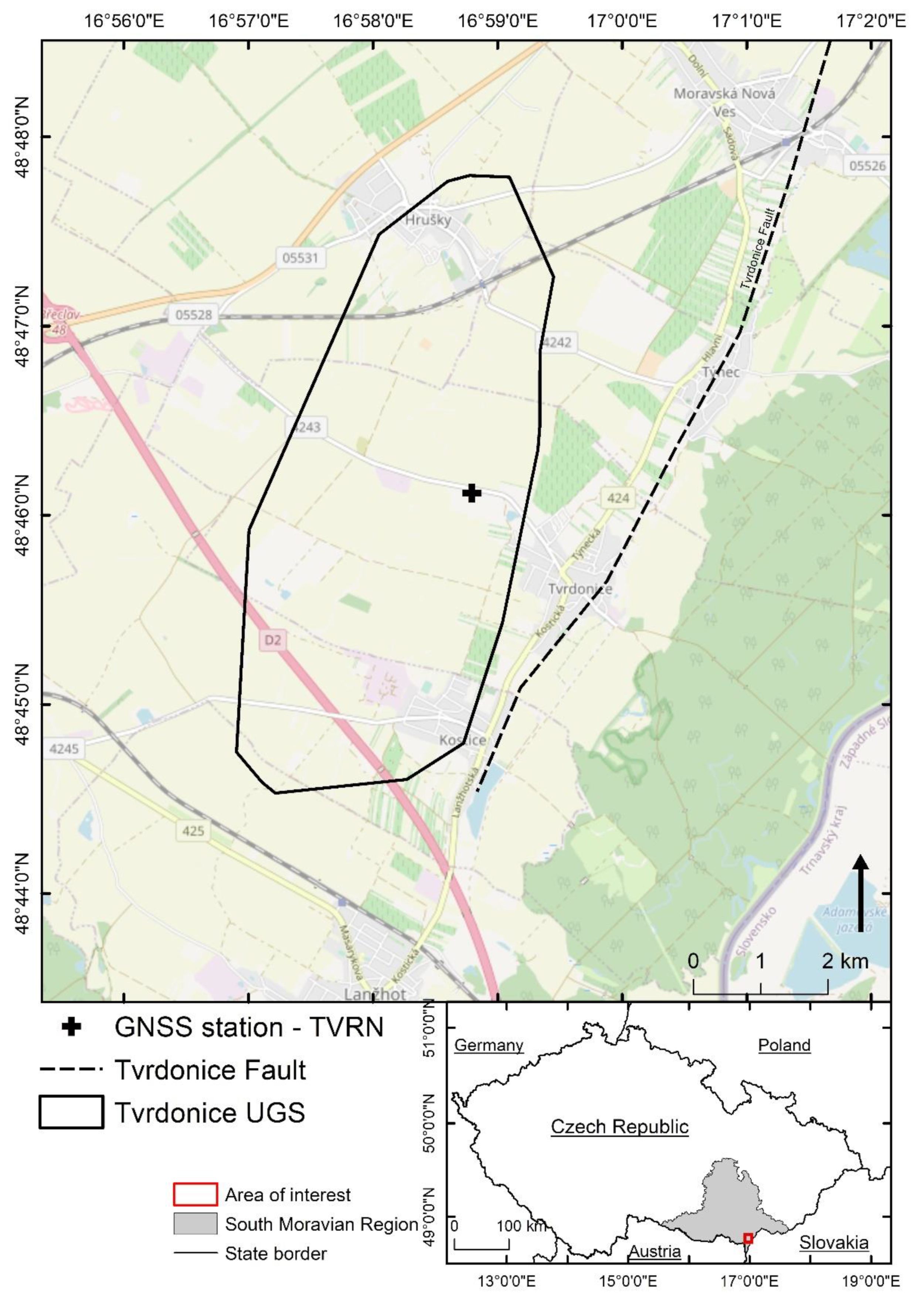
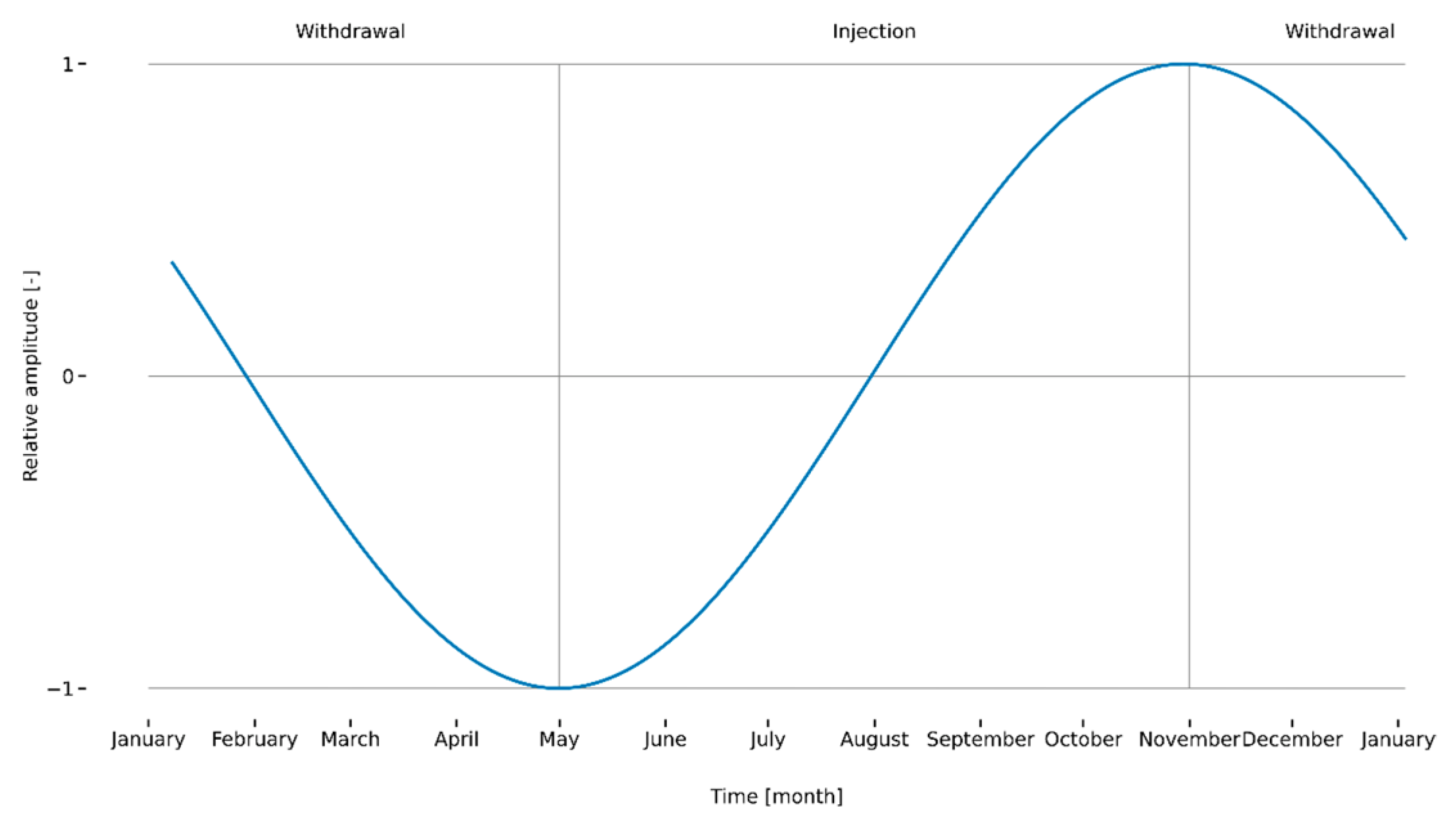
Horizontal terrain displacements induced by the injection/withdrawal of natural gas head toward the place with the most significant pressure drop, i.e., roughly to the center of the UGS (or perpendicular to the longitudinal axis of the UGS in the case of an elongated structure, as in the studied Tvrdonice UGS) during the withdrawal, and in the opposite direction from the center of the UGS at the time of injection. The magnitude of displacement and the size of the affected area are influenced by the deposition depth of the UGS storage structure and its geometry and the geomechanical properties of the storage structure and surrounding rocks, as well as changes in pore pressure in the storage structure during the injection/withdrawal cycle [10].
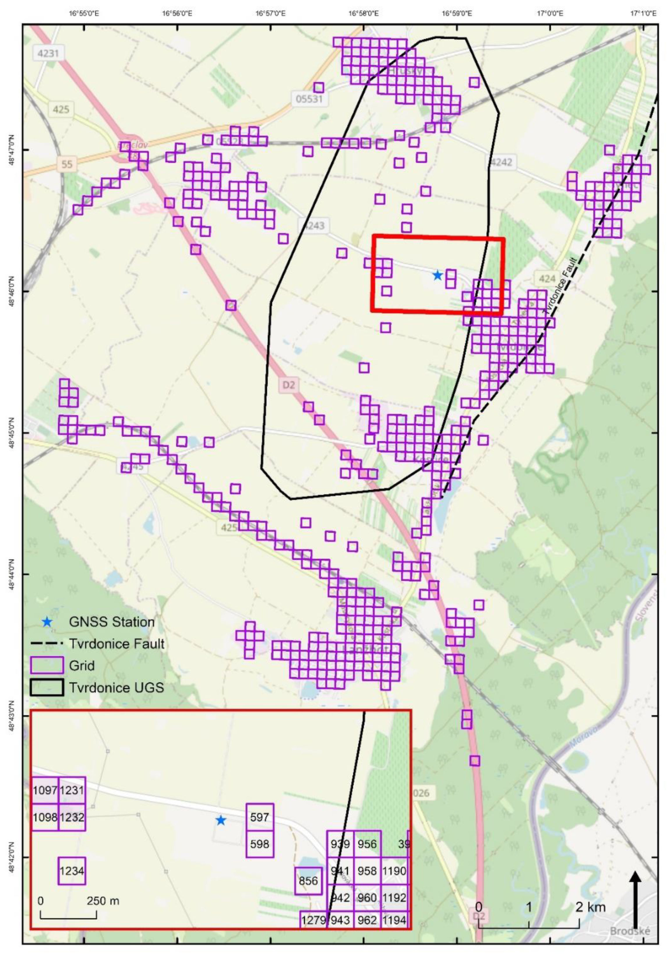
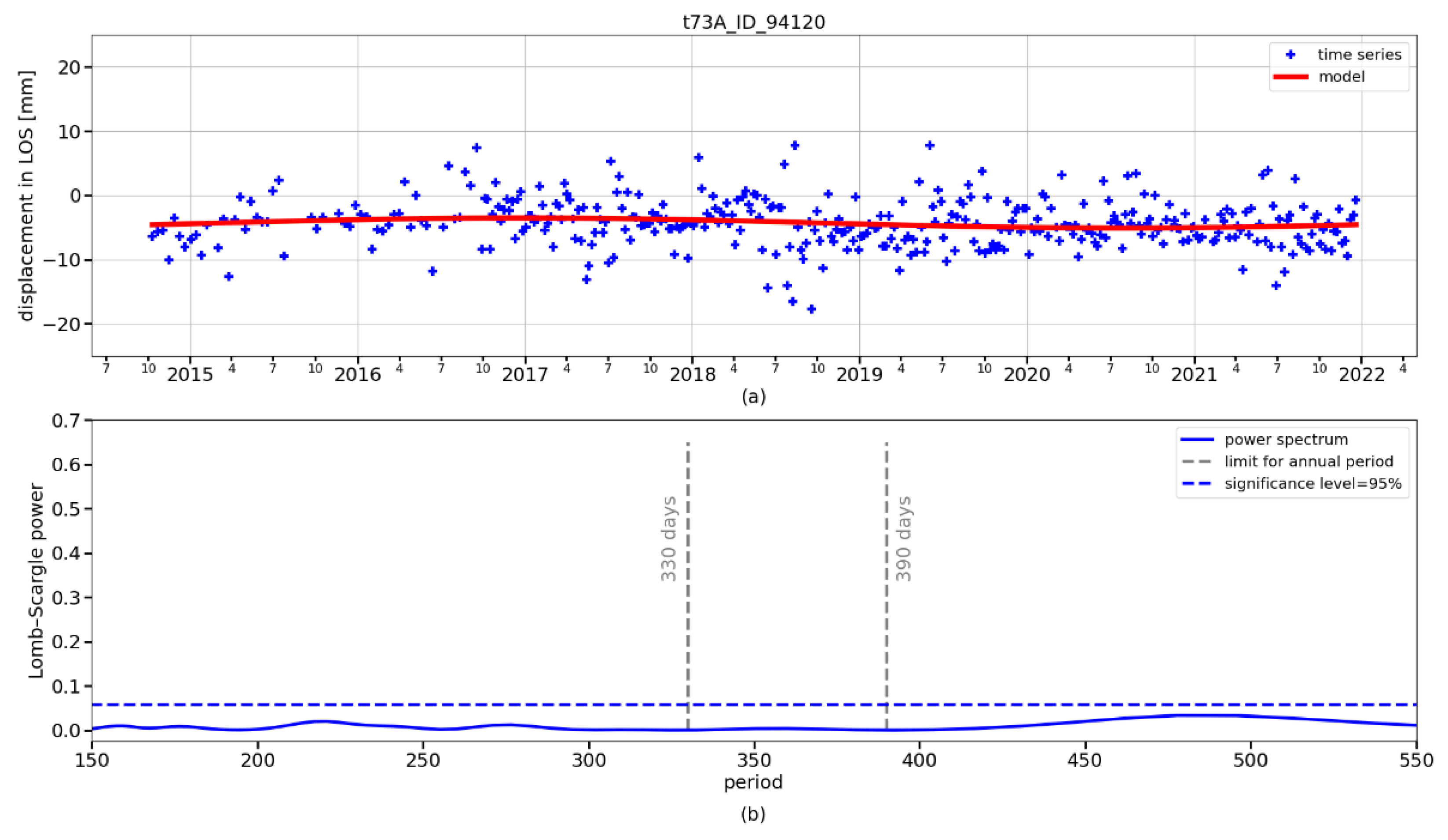
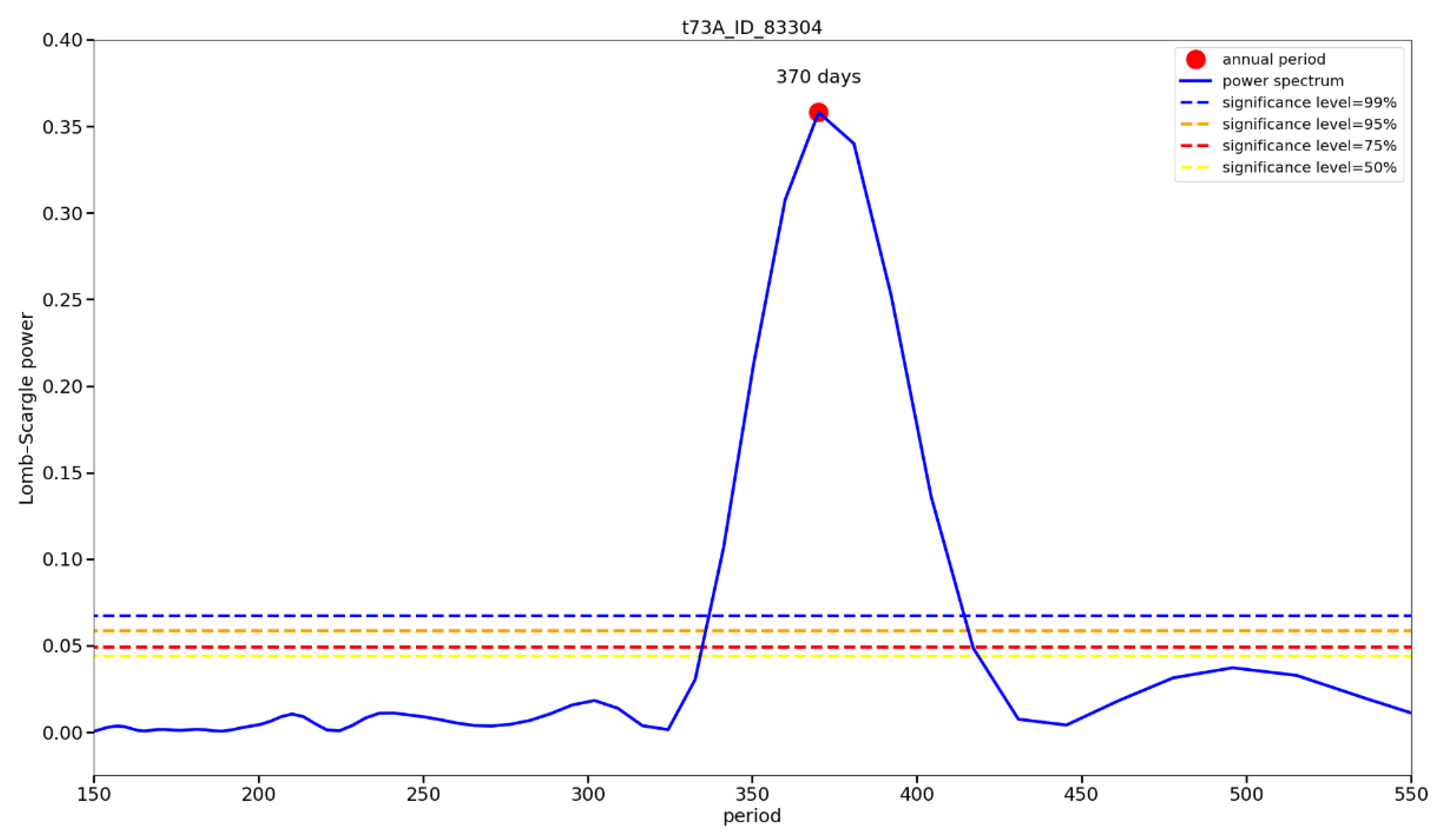
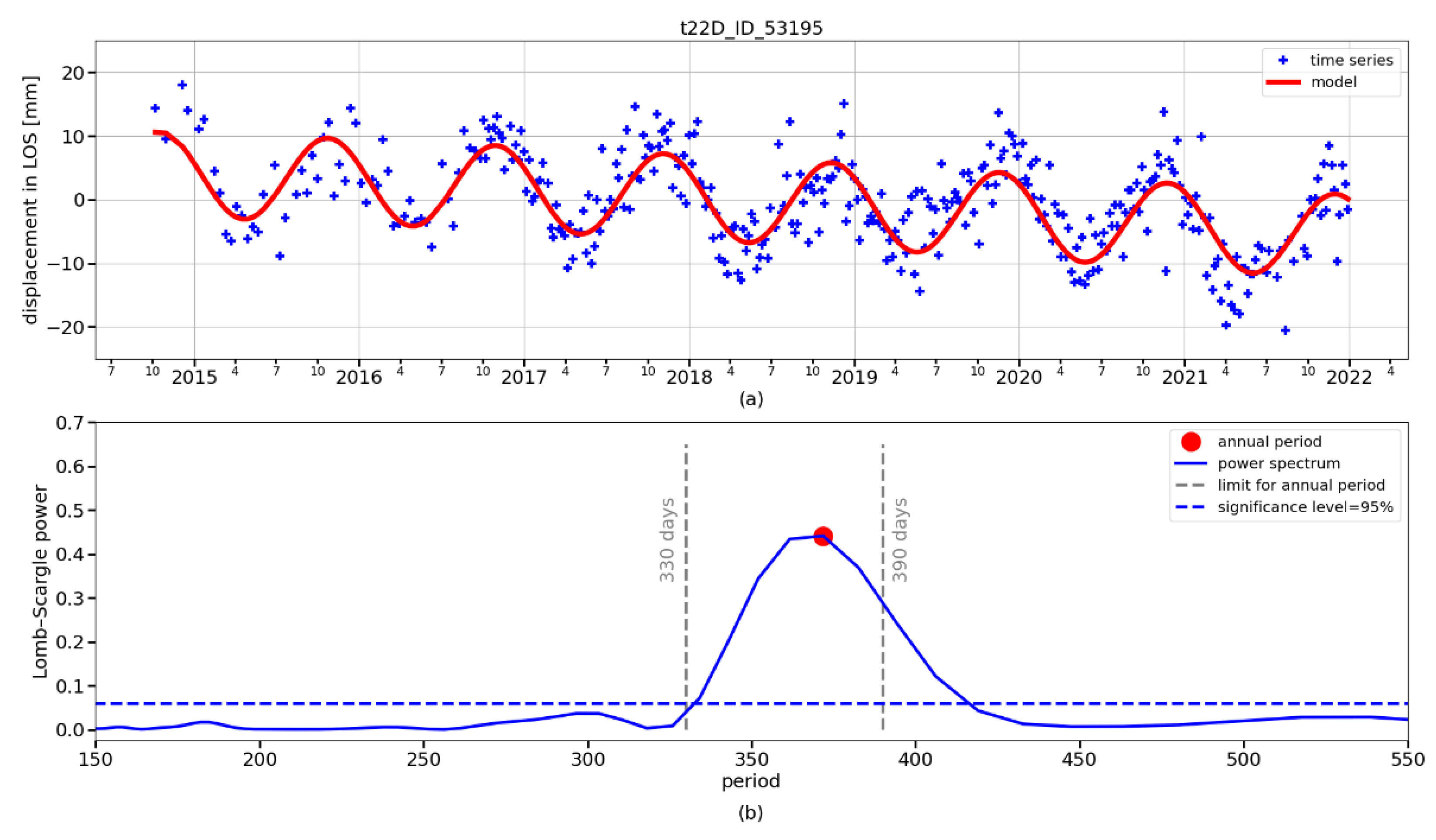
Our research was focused on a comprehensive area evaluation of periodic horizontal (E–W component) and vertical (U–D component) displacements over the selected UGS based on PSInSAR processing of freely available Sentinel-1 images. The analysis of their periodic character was based on obtaining E–W and U–D components by combined processing of time series of measurements in satellite line of sight (LOS) taken on ascending and descending tracks. For their necessary conversion to the same time frame, we used the Lomb–Scargle periodogram and models derived from it, with which we replaced the original time series. We also focused on the interpretation of the results in the context of UGS activity and the geological structure of the monitored area. The obtained results from monitoring the displacements of the Earth’s surface were validated against independent GNSS measurements.

2. Materials and Methods

2.1. Area of Interest

The area of the Tvrdonice UGS, located in the Czech Republic in southern Moravia near the borders of Slovakia and Austria, was selected for our study. It is in the relatively flat terrain of the northern outcrop of the Vienna Basin, which is filled with sediments of the Middle and Upper Miocene. It is known for the abundant occurrence of smaller deposits of lignite, oil, and gas [25]. The Tvrdonice UGS itself is built in a depleted oil and gas reservoir. Storage horizons are located at 1050 to 1500 m below the surface. The storage structure is a semi-domed trap elongated in the north-northeast–south-southwest direction. It is bordered from the east-southeast by the Lanžhot-Hrušecký fault, and on the opposite side, it gradually wedges towards the west-northwest. The UGS was commissioned in 1973 (https://www.rwe-gasstorage.cz/o-nas/nase-zasobniky/Tvrdonice (accessed on 22 May 2022)). 111 injection/withdrawal and monitoring wells are located on the UGS territory (http://muzeumropy.cz/tvrdonice/ (accessed on 22 May 2022)). A permanent GNSS reference station (Figure 1) was established near the center of the UGS for our research.
We compiled a theoretical filling curve for the UGS, verified by the course of fullness cycles of the so-called virtual UGS defined for the Czech Republic [26]. The whole cycle usually starts at the turn of April to May, initiating with gas injection into the UGS, and the injection is usually over at the turn of October to November, when withdrawal starts. Figure 2 displays the theoretical course of the injection and withdrawal cycle at the UGS [27].
However, the actual start and end of the injection or withdrawal depend on current natural gas consumption and can significantly differ from the given dates. For example, from 2011 to 2022, the minimum fullness of the virtual UGS ranged from 26 March to 1 May, and the maximum fullness ranged from 6 October to 9 December. Therefore, the working cycle period may not be exactly 365 days; in our case, it fluctuated from 342 to 388 days [26].

2.2. Satellite Radar Data Used

Satellite radar data from the Sentinel-1 mission are available for the area of interest (Tvrdonice UGS) from ascending track A73 and descending tracks D22 and D124 (Table 1). Our monitoring was realized for the period from October 2014 until December 2021. Data were collected in 12- or 6-day intervals depending on satellite availability. There were also few gaps in the data due to missing or damaged images. Figure A1 in Appendix A shows star graphs displaying the temporal/perpendicular baseline distribution between images for individual tracks.

2.3. Radar Interferometry

Satellite radar data processing by interferometry requires using at least two radar images. One is called the primary image, and all the others are called secondary images. The primary image is usually taken before the monitored event or at the beginning of the monitoring; all the others are secondary. Subsequent processing and results relate to the primary image. In the case of processing two images, it is possible to derive a digital surface model. When processing the time series of images, monitoring dynamic surface changes, such as glacier movement, landslides, mining works, mined areas, UGSes, and others, is possible [28].

2.3.1. Permanent Scatterer Interferometric Synthetic Aperture Radar

Permanent (persistent) scatterer interferometric synthetic aperture radar (PSInSAR) is one of the methods for processing a long time series of images (tens or hundreds of them). It is a technique where a time series of input radar images allows an identification of points representing permanent scatterers (PSes) of a radar signal. For each PS, it is possible to get a time series of its displacements in the direction of the satellite LOS with an accuracy of millimeters [29].
PSes are points on the terrain or infrastructure that are least affected by temporal and geometric decorrelations, i.e., pixels with stable backscattering of the radar signal over a long time. At the beginning of the processing, permanent scatterer candidates (PSCs; [30,31]) are selected based on the observed amplitude. Then, their displacement is estimated, together with other factors such as height correction, atmospheric contribution, and noise. Out of the pool of candidates, PSes are typically selected based on noise level, represented, e.g., by coherence. However, in the case of monitoring periodic motions, filtering according to coherence is not performed—PS points exhibit lower coherence precisely with respect to periodic motions, and therefore they would be excluded.
PSInSAR technique is implemented, for example, as open-source in SALSIT (small area least-squares InSAR tool; https://www.insar.cz/salsit.html (accessed on 22 May 2022)) and StaMPS (Stanford Method for Persistent Scatterers; https://github.com/dbekaert/StaMPS (accessed on 22 May 2022), or in the commercial processing software SARPROZ (SAR PROcessing tool by periZ; https://www.sarproz.com/ (accessed on 22 May 2022)).
The implementation in SALSIT was chosen for our processing. The pre-processing took place in SNAP (Sentinel Application Platform; https://step.esa.int/main/toolboxes/snap/ (accessed on 22 May 2022)), a software tool for data processing of the Sentinel program developed by the European Space Agency (ESA).

2.3.2. Pre-Processing and Processing PSInSAR

InSAR pre-processing and the following processing were performed burst-wise. Image coregistration was performed in the SNAP software, using a pre-defined XML graph (see Figure 3). The coregistration was performed based purely on precise orbit information. All images were coregistered with regard to the primary image, and interferograms were also created with regard to the primary image. PsInSAR processing was then performed in octave-based SALSIT software.
Atmospheric disturbance is characterized as slowly changing in space and quickly changing in time. Atmospheric delay is estimated based on the phase residues from the preliminary processing. Atmospheric delay subtraction was performed after the atmospheric phase determination. The estimated atmospheric delay was subtracted from the original coregistered interferograms.
Generally, the SALSIT was run three times with slightly different parameters and inputs:
  • PS processing for points with the highest quality;
  • Atmospheric delay estimation based on the residues estimated on these points, atmospheric delay subtraction;
  • PS processing for the same point set;
  • Densification of the PS network: processing lower-quality points with regard to high-quality points in their vicinity.
Displacement standard deviation (S0 [mm]) was calculated for individual points during SW SALSIT processing. These deviations are affected by unwrap errors and periodic point movement, as SALSIT compares the measured data with a linear model (see Table 2).

2.3.3. Satellite Line of Sight Geometry

The limiting factor of radar interferometry is that it is only able to measure terrain motion towards or away from the satellite [14]. Therefore, it allows for generating time series of displacements only in the satellite LOS direction. Unfortunately, this one-dimensional information does not always provide sufficient information to detect, e.g., potential disasters [17].
Let us suppose measurements in LOS from ascending and descending tracks are available. Theoretically, it is possible to create a local displacement field for the monitored area in all three dimensions, which can significantly improve our understanding of the behavior of the studied area [10]. In practice, because current SAR satellites are located only on sub-polar solar-synchronous orbits and the LOS is perpendicular to the orbit, InSAR is very sensitive to U–D and E–W shifts but is almost insensitive to shifts in the N–S direction [2,10,11,32].
To make the combined processing of LOSes from ascending and descending tracks possible, it is necessary to resample measurements that take place at different times and different PS points to the same places and at the same times [4]. In the spatial domain, a regular grid of patches is used for resampling, with the fact that only those patches that contain at least one measurement in the ascending and one in the descending track are processed.
Resampling in the time domain was ensured by substituting the original time series with their models obtained from the Lomb–Scargle periodogram (LSP; see below) and representing only the periodic component. These models derived time series values for the same time points with a step of 6 days [33].
The great advantage of this approach is that it allows even merging of data acquired by completely different SAR sensors [10,24].
InSAR measurements are expressed as a shift in the satellite LOS. The LOS geometry is defined by the incidence angle θ (angle between the local zenith and the satellite view) and the heading (azimuth) of the satellite α (Figure 4).
The displacement of a point located on the terrain surface measured by InSAR is influenced by E–W and U–D components only. Therefore, according to [4,11,34], we can express the shift in the LOS direction as follows:
D L O S = D E W S E W + D U D S U D ,
where D L O S is the shift in the LOS direction, D E W and D U D are the shifts in the respective directions, and S E W and S U D are the sensitivity parameters for the particular directions.
For satellites on ascending and descending tracks, we can write [34]:
D L O S ,   a s c D L O S ,   d s c = S E W , a s c S U D , a s c S E W ,   d s c S U D , d s c D E W D U D
Sensitivity parameters for particular directions can be written as sensitivity matrix S [34]:
S = sin θ a s c cos α a s c cos θ a s c sin θ d s c cos α d s c cos θ d s c
and Equation (2) as:
D L O S , a s c D L O S , d s c = S D E W D U D
Teatini et al., in [10], have shown that when there is a motion in the N–S direction of 10 mm, the U–D component is subject to an error of up to 1 mm, and the effect on the E–W component is less than 0.1 mm. Therefore, neglecting the N–S component does not usually affect the estimates of the other two components.
From Equation (4), it is possible to deduce:
D E W D U D = S 1 D L O S , a s c D L O S , d s c
For combined processing of data from ascending and descending tracks, a primary grid was created for the Tvrdonice UGS area and its surroundings, which corresponded to the extent of PSes from track D22, with a patch size of 120 × 120 m. From this grid, we deleted patches that did not contain at least one PS from the measured ascending and descending tracks, and on the contrary, we manually added patches that did not match the patches of the original grid but contained at least the required number of PS points from both directions of scanning. These patches were defined so that they did not overlap with others. An example is cell 856 in Figure 5.
Data for individual tracks were recorded at different times. In order to achieve the coincidence of the processed data, the data for individual directions were substituted by a model from which the searched values were interpolated. The models were calculated by the LSP (see Section 2.3.3.) [33].
The reference calendar date 15 July 2018 was chosen in the calculation. The value of this calendar date for each PS time series was subtracted from the entire time series, i.e., this date was set to zero. Subsequently, the time series corrected this way were input into the calculation. The calculation was performed separately for each date in the time series.

2.3.4. Extraction of the Periodic Component from the PS Time Series

We needed to obtain information related to the periodic motion of the terrain caused by the cyclic activity of the UGS by extracting the periodic component from data describing the behavior of individual PS points.
The data relating to each PS can be viewed as a time series of measurements. Each time series can be split into several components [35]: the long-term trend, the seasonal component, the periodic component, and the irregular component. We did not anticipate a long-term trend in the case of time series related to UGS. The monitored UGS went through dozens of injection/withdrawal cycles, so it can be assumed that the area is already stabilized; time series visualizations confirmed this (see Figure 6 and Figure 7). If it still appeared in the data, it was eliminated in subsequent processing.
The seasonal component is caused by annual temperature changes and is almost synchronous with the periodic component, carrying information about the periodic behavior of the terrain above and around the UGS caused by its cyclical activity. Therefore, these two components cannot be easily distinguished. On the other hand, as follows from [27], the seasonal component is negligible compared to the periodic component, so we did not consider it further.
The irregular component (noise) can be removed, for example, by a moving average (provided that unwrapping errors [36] do not occur in the data or are removed). This step is especially very suitable for visualization needs [26].
The subject of our interest was periodic terrain motions caused by cyclic injection/withdrawal of natural gas to/from the UGS and represented by the periodic component of the processed time series. Therefore, we needed to extract this component from the time series. For this purpose, we could use fast Fourier transformation (FFT), which can break down the periodic component into individual partial periodic signals—partial components. FFT is especially suitable for time series with regular sampling. In our case, however, this condition was not met: the sampling step in the processed data changed (6 or 12 days depending on the availability of satellites), and there are also gaps in the time series due to unavailable data. Therefore, we looked for a suitable method applicable to an irregularly sampled time series. We found it in the Lomb–Scargle periodogram (LSP) ([37,38] in [39]). The LSP makes it possible to find and test the significance of individual constituents of the periodic component contained in an irregularly sampled signal burdened by noise. The result of the processing was a periodogram representing the periodic signal components (Figure 8).
The peaks of the periodogram correspond to the significant frequencies of the signal, and therefore the resulting periodogram can be used to construct a model that best matches the data. For each significant constituent of the periodic component, it is possible to construct a model in the form of a sinusoid, the amplitude of which corresponds to the degree of its agreement with the data (using library LombScargle, https://docs.astropy.org/en/stable/timeseries/lombscargle.html (accessed on 22 May 2022)). Theoretically, it is possible to construct a model as the sum of individual sinusoidal models. However, in our case, only one sinusoidal model was used, corresponding to a period approaching one year. It thus represented the periodic component of the signal, which was the subject of our interest. After all, its power was always the largest in the data we processed (with a level of significance higher than 95%); significant periods of 6 and 12 days, often found in the data and corresponding to sampling periods, were neglected. No other significant period occurred in the data of any processed PS point (Figure 8).

2.4. GNSS Measurements

2.4.1. GNSS Data Collection and Processing

Data obtained by GNSS can be used to determine the validity of the LOS decomposition results into U–D and E–W components. The GNSS reference station abbreviated TVRN was installed on 8 October 2019 on a building in an industrial area situated approximately 750 m east of the main UGS ground facility, nearly in the center of the UGS (see Figure 1).
The GNSS reference station TVRN was equipped with a geodetic-grade GNSS receiver (TPS GB-1000) with a choke-ring antenna (TPSCR.G3 TPSH). The receiver was placed inside a building to log raw observation data from GPS and GLONASS satellites in a 30 s interval. GNSS data collection was running smoothly during the measurement period, with occasional outages, as shown in Table 3. Continuous data collection was realized until the end of April 2022; however, only the data to 8 February 2022 were processed for this study.
GNSS data processing was realized in Bernese GNSS Software 5.2 [40] using the network solution based on double-differenced observations. Basic information about the processing settings is given in Table 4. A regional network of 20 GNSS stations across Europe was set up (see Figure 9). Stations with longer distances from the Czech Republic were chosen to de-correlate station heights and tropospheric parameters.

2.4.2. Conversion of GNSS Measurements to PSInSAR LOS

To compare GNSS and PSInSAR, it was necessary to convert their outputs to comparable quantities and directions. In principle, it is possible to compare E–W and U–D from InSAR with E–W and U–D from GNSS or to convert 3D GNSS measurements to 1D LOSes and compare them with LOSes from InSAR [8,42].
The comparison of E–W and U–D can be made directly. If comparing in the LOS direction, the D G N S S has to be converted into D L O S using Equation (1). For comparison, the time series of both methods must be corrected by their average so that the averages of the compared time series are equal to zero.

3. Results

3.1. Time Series of GNSS Data

At the time of the GNSS reference station installation, the UGS was probably filled with gas and prepared for the 2019/2020 heating season. Higher altitude of terrain (and GNSS reference station; see Figure 10) could be expected during the first months of the processed period, followed by a decrease in height related to gas withdrawal during winter and early spring. Later, during summer and the beginning of autumn, a rise in terrain and GNSS reference station height could be expected related to gas injection in preparation for the heating season.
To check the possibility of horizontal motion over the UGS, we plotted time series of position changes of the TVRN and other processed GNSS stations in the directions N–S and E–W. Figure 10 shows these time series together with height changes for GNSS stations TVRN, TUBO (located in Brno city, approximately 50 km from TVRN), GOPE (located in Ondřejov city, approximately 205 km from TVRN), and CFRM (located in Frydek-Mistek, approximately 140 km from TVRN). This figure clearly shows that the position of TVRN was periodically changing in latitude, longitude, and height, while the position of the other three stations was not changing systematically. As the periodic motion was found only for station TVRN out of all twenty processed GNSS stations, it probably corresponded to actual station motion.
The colder the winter is, the higher the expected gas consumption for heating, and therefore higher terrain height changes occur. Figure 11 shows mean monthly temperatures in the southern Moravian region between January 2019 and April 2022. During winter 2019/2020 and early spring 2020, temperatures were often well above the long-term average. Overall, the 2019/2020 winter was mild. On the contrary, temperatures were around or below the long-term average during 2021. The described situation not only related to the southern Moravia region but to the whole Czech Republic and Europe (see, e.g., https://www.eumetsat.int/february-2021-very-cold-first-half-europe-and-north-america (accessed on 7 June 2022)). It meant higher gas consumption from the Tvrdonice UGS and, therefore, higher terrain changes could happen in the second half of the 2020/2021 heating season compared to the 2019/2020 one. However, this is only an assumption as data describing the actual situation within the UGS were unfortunately not available for this study.

3.2. Comparison of GNSS with PSInSAR in LOS

In order to take into account both vertical and horizontal motion in the studied area and properly compare the results of InSAR and GNSS techniques, GNSS TVRN’s 3D position changes were converted into a satellite LOS direction of all processed Sentinel-1 tracks. Therefore, the GNSS TVRN results evaluated below are as they would be seen by Sentinel-1 satellites from their tracks. Moreover, GNSS time series were smoothed by a floating average computed over 35 days to compare them with the PSInSAR time series.
The GNSS time series was converted to LOS according to Equation (1). To convert to LOS, we needed to know the heading (azimuth) α and the incidence angle θ. We used the heading available in the primary image annotation for our calculation. The incidence angle was calculated using the position of the station and the ephemeris in the primary image annotation. From both angles, we could derive the necessary sensitivity parameter for each direction (Table 5).
Figure 12 shows the time series in LOS for the GNSS and InSAR outputs for all three tracks. Since there was no PS point near the GNSS station in the ascending track, we chose patch 597 at the GNSS station for comparison—see Figure 5.
For individual tracks, we calculated RMS errors and correlation coefficients between GNSS and PSInSAR results (see Table 6).
It can be seen from Figure 12 and Table 6 that for the LOS for track A73, the horizontal and vertical components of the motion compensated for each other due to the geometry of the setting, in contrast to both descending tracks. The RMSEs for the LOSs came out to around 2.75 mm for all tracks. The correlation coefficient reached almost 1.0 in the descending tracks, while no correlation between the two techniques was found in the A73 track. This situation can be attributed to the minimal absolute range of values (no periodicity) in track A73, where the statistical evaluation was more influenced by noise in both the InSAR and GNSS time series. A comparison of displacement measurement between GNSS and PSInSAR can also be shown in the scatter plot—see Figure A2 in Appendix B.
To further study the behavior of PS points from both tracks and confirm the results shown above, we have plotted their time series over an entire processed InSAR period spanning almost seven years. In track A73, no statistically significant annual period was found using the Lomb–Scargle periodogram for the evaluated PS point (see Figure 6 showing point 94,120). On the other hand, a statistically significant annual period was identified for both points from the D124 and D22 tracks (see Figure 7 and Figure 13 showing point 173,697 and point 53,195, respectively); for all point locations, see Figure 14.

3.3. Comparison of E–W Displacement from PSInSAR and GNSS

As can be seen from Table 1, the modelled data had to be truncated in the range from 14 October 2014 to 18 December 2021 (which corresponds to the most extended time series covered by all tracks). The model derived from the periodogram can be seen in Figure 13, marked by a red line.
In the next step, the displacement in the U–D and E–W directions was calculated for each patch with PSes according to Equation (4). A total of 501 patches were processed above the UGS and in a four-kilometer neighborhood around the reservoir (Figure 5).
After conversion to the U–D and E–W directions, we compared the values from InSAR with the measured values at the TVRN GNSS station. The comparison was made for the period from 14 October 2019 to 18 December 2021, which was covered by both methods. The time series for the GNSS station was resampled to the PSInSAR interval and time step. We have all displacement directions for the GNSS time series, i.e., E–W, N–S, and U–D. However, we processed only the E–W and U–D components.
For comparison, the GNSS time series were smoothed using a floating average with a window of 35 days. The result for patch 597 is shown in Figure 15.
When visually evaluating the result of the PS model, it can be seen that the vertical component in the GNSS measurement is noisier; therefore, a higher RMSE will be based on it. In the vertical (horizontal) direction, the RMSE between GNSS and PSINSAR was 2.35 (1.75) mm (Table 7). Such low RMSEs can be affected by the chosen PSInSAR conversion method, where instead of the measured data, we used a model, and thus the majority of the noise in the PSInSAR measurement was removed.
Each patch displays a separate time series of vertical and horizontal motion. There may be differences between close patches corresponding to noise. For animation creation purposes, it was advisable to smooth these time series in space; we used the spatial window of 3 × 3 patches. In Figure 16, we have displayed two images for the vertical time series, where Figure 16a shows the situation at the end of October 2015, when the UGS should be full. Figure 16b shows the situation at the end of April 2016, when the UGS was supposed to be empty. For horizontal motion, it can be seen that when the UGS is full, the right area (green) shifts to the east (Figure 16c). When the UGS is empty, this area moves to the west (Figure 16d). When combining E–W and U–D motions, we can tell that there is an “inflation” when filling the UGS, i.e., the area above the UGS uplifts and moves away from the UGS center. In the withdrawal period, the area above the UGS subsides and moves towards the UGS center. Supplementary Materials published on the web contain animations of E–W displacement evolution over 2015–2022 and U–D displacement evolution over 2015–2022.

4. Discussion and Conclusions

Our research was focused on assessing the possibility of aerial monitoring of periodic vertical and horizontal motions of the terrain above a UGS using the PSInSAR technique and on their interpretation with the UGS work cycle and considering the area’s geological structure. The first aspect concerns, in particular, the terrain above the UGS, the second also the broader surroundings of the UGS, where the motions of the terrain can induce further changes, for example, reactivating faults.
This study showed that PSInSAR is suitable for this purpose. We have found that the combined processing of PSInSAR outputs for ascending and descending tracks is suitable for the aerial monitoring of periodic terrain motions and breaking them down into E–W and U–D components (see attached animations on the web). The outputs of this processing provide a good idea of the behavior of the terrain above and in the vicinity of the UGS, and this behavior is consistent with the cyclic injection/withdrawal the UGS is subjected to.
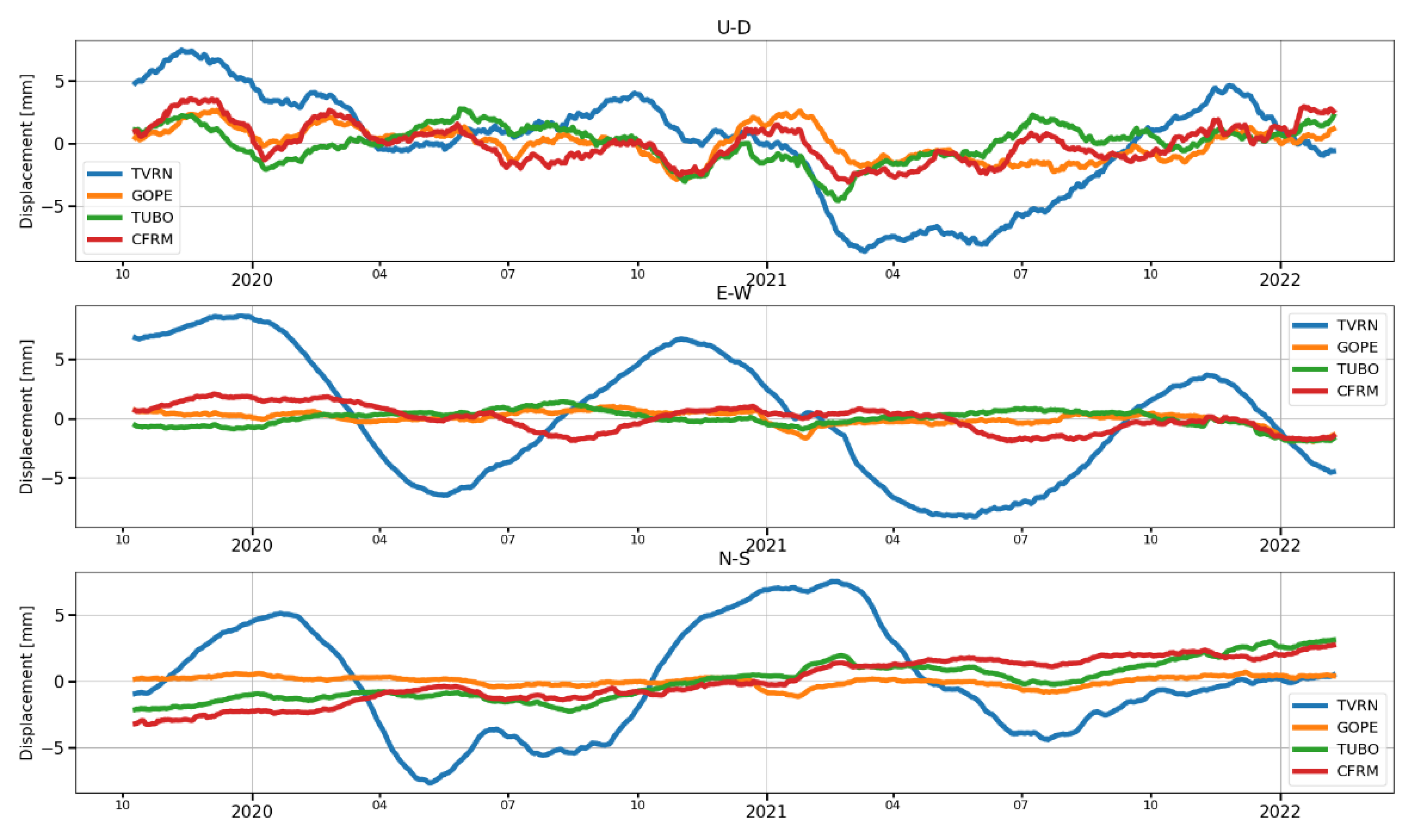
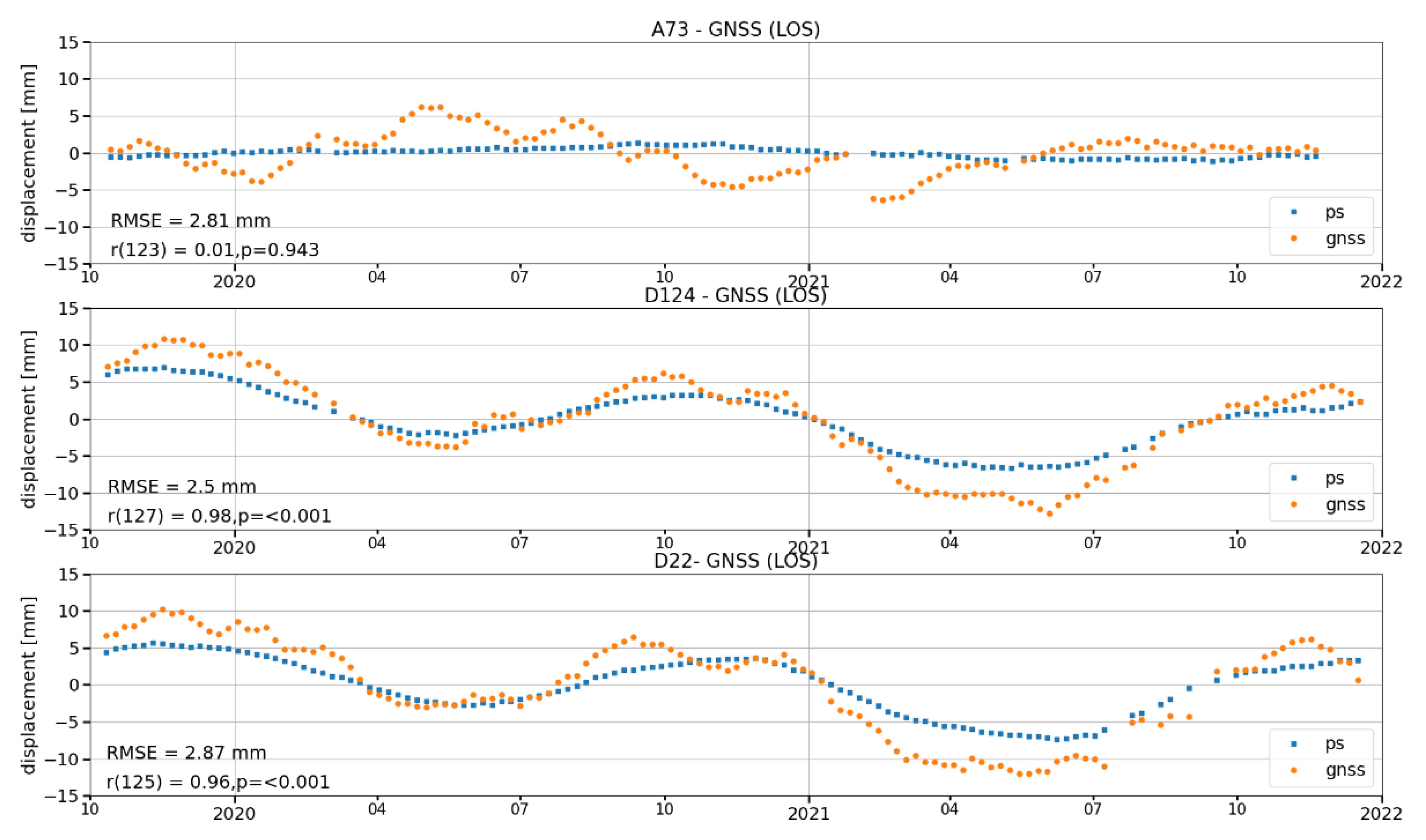
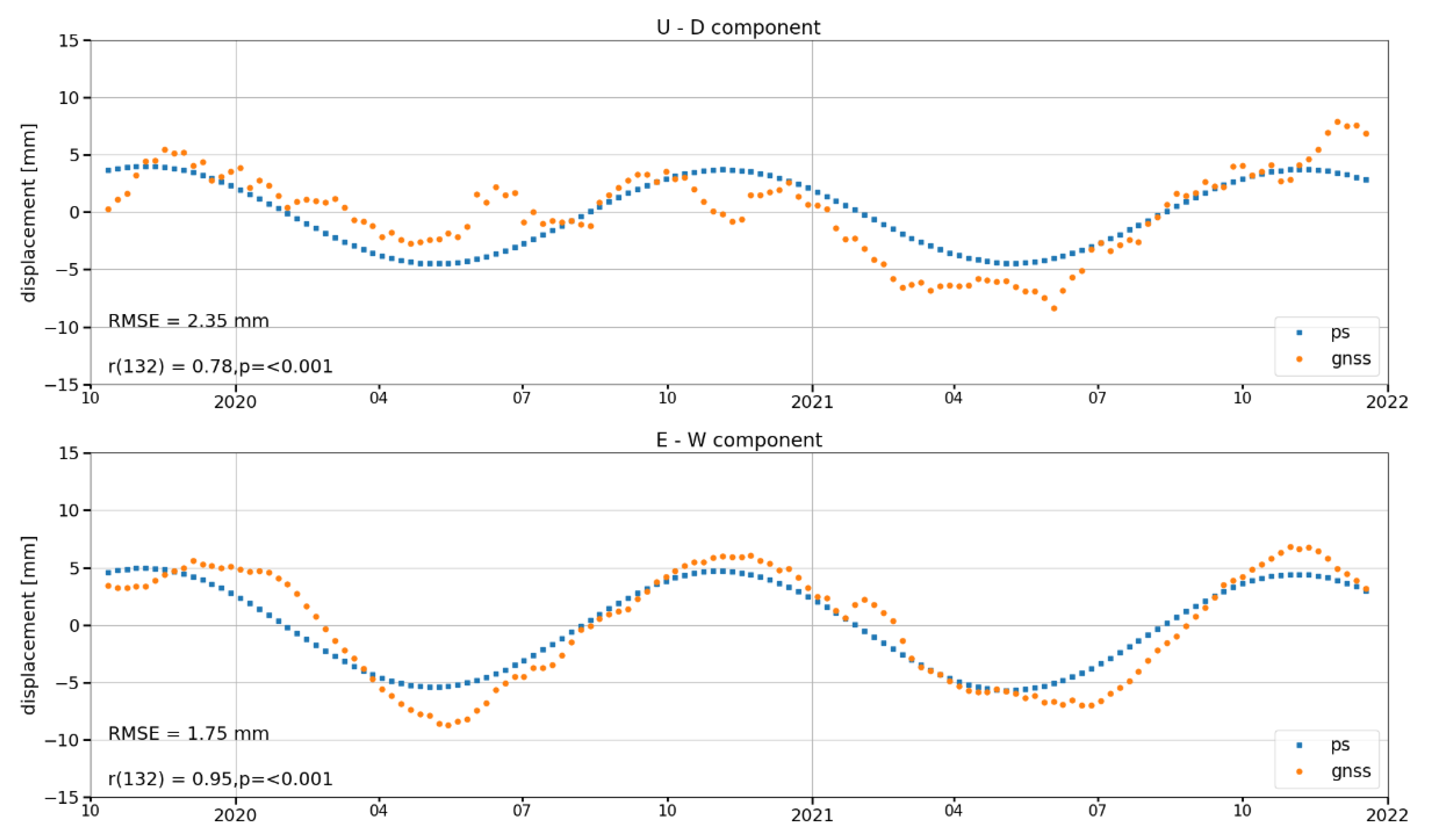
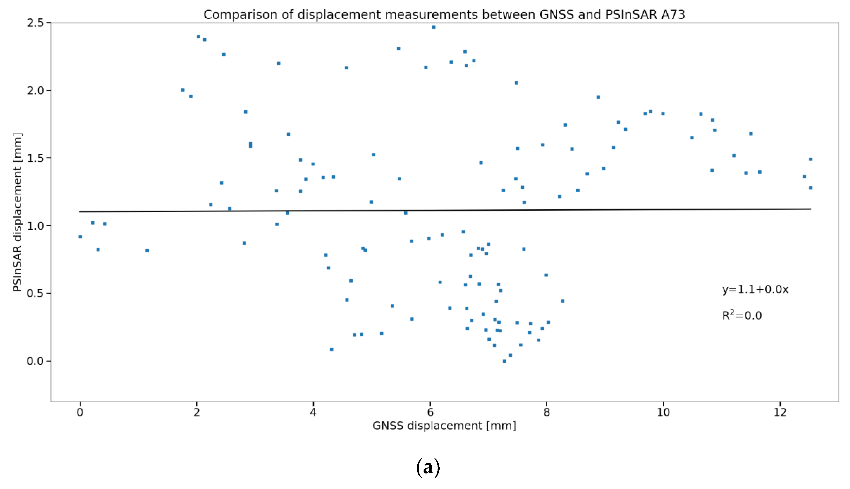
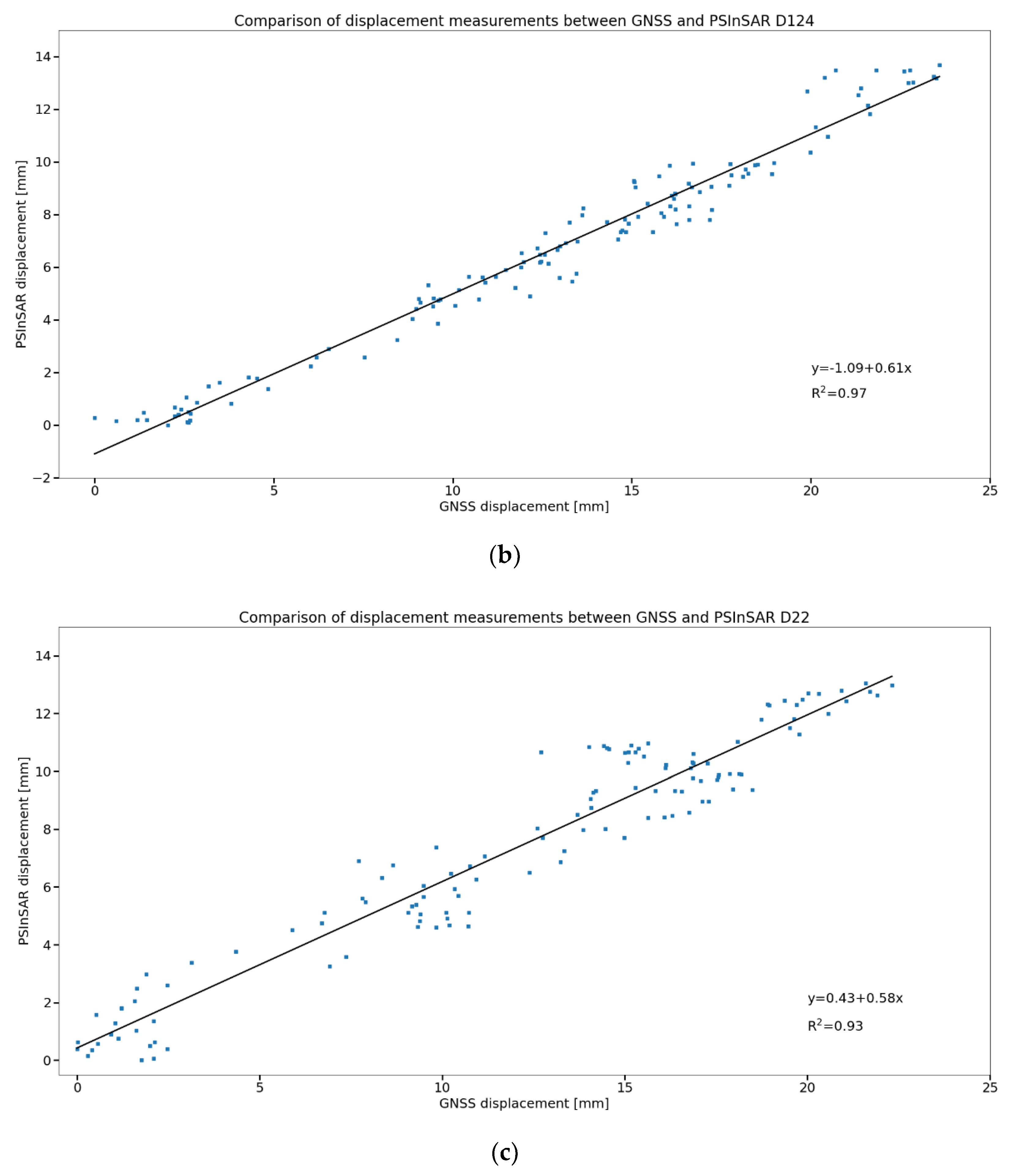
The evaluated motions in the E–W and U–D directions were also verified by independent measurements using a permanent GNSS station above the UGS. The results showed good agreement in the evaluation of motions by both methods (correlation coefficient between LOS from both methods based on descending track was on average 0.97, with an RMSE of 2.70 mm; in the case of E–W correlation the coefficient 0.95 was and the RMSE was 1.75 mm; for U–D it was 0.78 and 2.35 mm; and allow interpretation of aerial evaluation of E–W component from InSAR concerning the geology of the area and the periodic activity of UGS.
We found that the behavior of the terrain over the UGS was consistent with results published for other areas. Although these mainly related to monitoring linear shifts, they are also helpful for comparing our PSInSAR and GNSS measurements. Published works comparing the two methods were focused mainly on monitoring subsidence [1,2,11,18] or landslides [8,19,20,21]. We achieved the resulting accuracies, which are consistent with the published results. For example, in [1], the horizontal displacement rates measured by InSAR agreed with GPS measurements within 1.8 mm a year, and the vertical displacement rates agreed within 4.8 mm a year.
Studying periodic motion of the terrain surface using PSInSAR and their verification using GNSS has so far received little attention. Such studies have only recently begun to appear. For example, [24] dealt with cyclic motions above a UGS; its authors found the difference between the deformation rate of the GNSS reference station observations and the results of PSInSAR for Sentinel-1 tracks T114, T41, T19 to be 4.1 mm, 2.4 mm, and 3.1 mm a year, respectively. The InSAR and GNSS measurements were evaluated as consistent.
The orientation of the horizontal motions detected over the Tvrdonice UGS also followed the assumed terrain behavior described in [10], and they were also in agreement with [
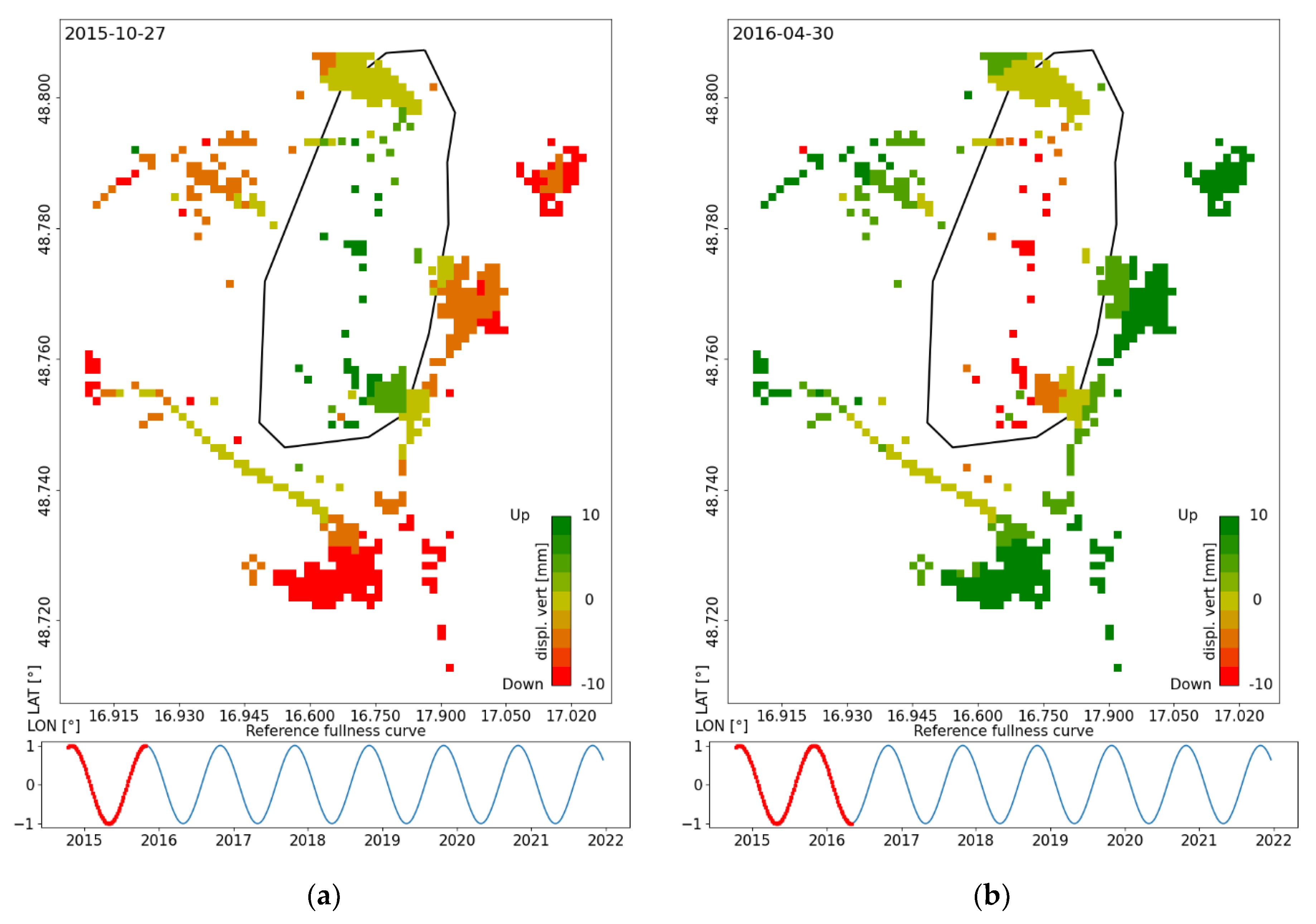
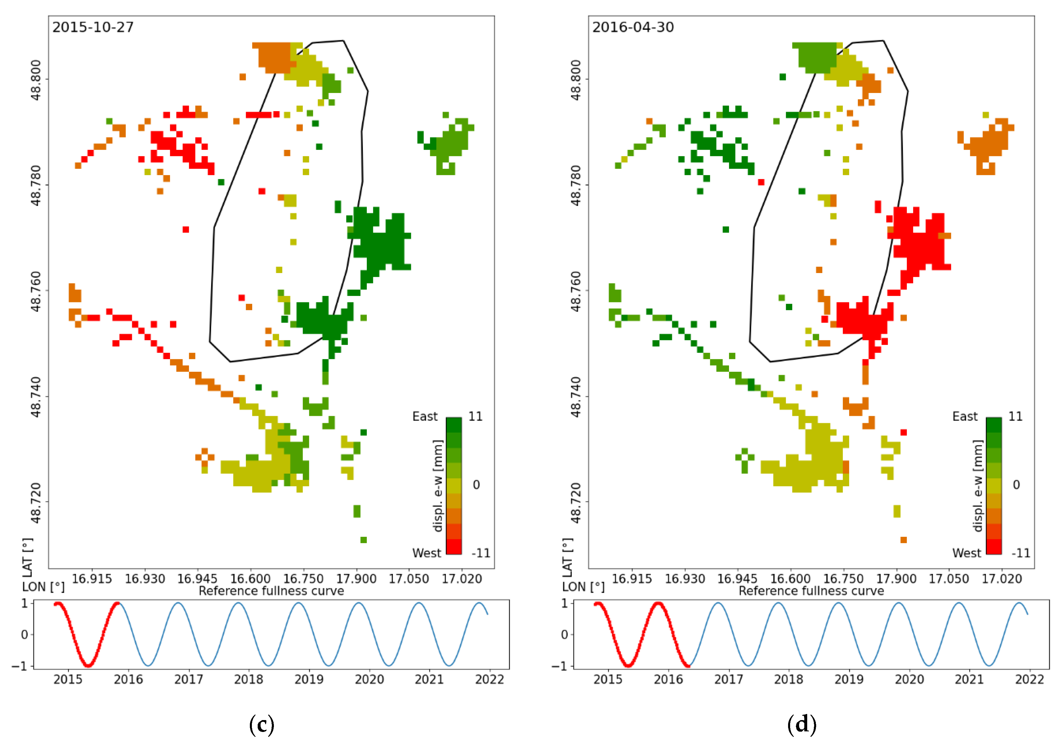
23], where the authors dealt with the 3D geomechanics of a UGS in northern Italy. During withdrawal, the terrain height decreased above the UGS, and the surface tended to move toward the center of the UGS; during injection, the direction of both motions was opposite.
The evaluated U–D motion agrees with the study presented in [27], which was based purely on evaluating motion in the LOS direction. In this study, the authors interpreted the different behavior of the area west of the Tvrdonice fault as a consequence of motion along this fault induced by the injection and withdrawal of natural gas to and from the Tvrdonice UGS. The obtained results were interpreted as that when the UGS was filled, the terrain rose above the UGS, but the area west of the Tvrdonice fault decreased in height due to slippage down along the fault.
A detailed evaluation of the motions broken down into U–D and E–W components confirms this assumption. Figure 16a,b shows that this region is really moving in the U–D direction in the antiphase to the injection/withdrawal cycle.
It can be assumed that systematic monitoring of UGSes could help identify degrading parts of the storage structure, non-standard well behavior, and reactivation of faults [1,2,3,4,5].
The achieved results gave a positive answer to our research question. The PSInSAR technique allows monitoring of periodic horizontal motions in the E–W direction. To further confirm the results, it would be interesting to compare the resulting curves of periodic shifts in the terrain surface with the curve of the fullness of the monitored UGS; however, these data are unavailable due to the protection of trade secrets. Only data for the so-called virtual storage are available, which represents a sum of the fullness of all UGSes located in the Czech Republic. However, it is impossible to derive the filling curve of the Tvrdonice UGS from this total curve.
Freely available Sentinel-1 mission data were used for this study, limiting the processing results quality due to their lower spatial resolution. In further research, it would be appropriate to use data from commercial radar satellites, which have a much higher spatial resolution and often provide long-time image series, allowing one to study UGSes for a long time into the past.

Supplementary Materials

The following supporting information can be downloaded at: https://www.mdpi.com/article/10.3390/rs14194898/s1, Video S1: E–W Displacement Evolution over 2015–2022; Video S2: U–D Displacement Evolution over 2015–2022.

Author Contributions

Conceptualization, P.R., M.K., J.S., I.H. and M.L.; methodology, I.H, J.S., M.K. and M.L.; software, J.S. and I.H.; validation, M.K. and I.H.; formal analysis, J.S. and M.K.; investigation, J.S., M.K. and P.R.; resources, M.K. and J.S.; data curation, J.S. and M.K.; writing—original draft preparation, P.R., J.S. and M.K.; writing—review and editing, P.R.; visualization, J.S.; supervision, P.R. and M.K.; project administration, M.K. and P.R.; funding acquisition, M.K., P.R. and M.L. All authors have read and agreed to the published version of the manuscript.

Funding

This research was funded by the European Space Agency, project Earth Observation Automated Monitoring Open Platform n. AO/1-9090/17/NL/MP (https://incubed.phi.esa.int/portfolio/cgi-satsight/ (accessed on 29 November 2021)).

Data Availability Statement

Sentinel-1 imagery is freely available to all users; see https://sentinels.copernicus.eu/web/sentinel/missions/sentinel-1/data-products (accessed on 29 November 2021).

Conflicts of Interest

The authors declare no conflict of interest.

Appendix A

Figure A1. Star graphs showing the temporal/perpendicular baseline distribution between images for the track (a) A73, (b) D22, and (c) D124.
Remotesensing 14 04898 g0a1aRemotesensing 14 04898 g0a1b

Appendix B

Figure A2. Comparison of displacement between GNSS and PSInSAR for track A73 (a), D127 (b), and D22 (c). The R2 value is the squared correlation coefficient between compared displacement measurements, and when R2 equals 1, the data being compared are the same. In our case, R2 is close to 1 for tracks D22 and D124, and for track A73 R2 = 0.
Remotesensing 14 04898 g0a2aRemotesensing 14 04898 g0a2b

References

  1. Klemm, H.; Quseimi, I.; Novali, F.; Ferretti, A.; Tamburini, A. Monitoring horizontal and vertical surface deformation over a hydrocarbon reservoir by PSInSAR. First Break. 2010, 28, 29–37. [Google Scholar] [CrossRef]
  2. Morgan, J.; Raval, S.; Macdonald, B.; Falorni, G.; Iannacone, J. Application of advanced InSAR techniques to detect vertical and horizontal displacements. In Proceedings of the 2013 International Symposium on Slope Stability in Open Pit Mining and Civil Engineering, Brisbane, Australia, 25–27 September 2013; Australian Centre for Geomechanics: Perth, Australia, 2013; pp. 829–840. [Google Scholar] [CrossRef]
  3. Ferretti, A.; Tamburini, A.; Novali, F.; Fumagali, A.; Falorni, G.; Rucci, A. Impact of high resolution radar imagery on reservoir monitoring. Energy Procedia 2011, 4, 3465–3471. [Google Scholar] [CrossRef]
  4. Tamburini, A.; Del Conte, S.; Ferretti, A.; Cespa, S. Advanced Satellite InSAR Technology For Fault Analysis and Tectonic Setting Assessment. Application To Reservoir Management and Monitoring. In Proceedings of the International Petroleum Technology Conference, Kuala Lumpur, Malaysia, 10–12 December 2014. [Google Scholar] [CrossRef]
  5. Bayramov, E.; Buchroithner, M.; Kada, M.; Zhuniskenov, Y. Quantitative Assessment of Vertical and Horizontal Deformations Derived by 3D and 2D Decompositions of InSAR Line-of-Sight Measurements to Supplement Industry Surveillance Programs in the Tengiz Oilfield (Kazakhstan). Remote Sens. 2021, 13, 2579. [Google Scholar] [CrossRef]
  6. Vassallo, R.; Calcaterra, S.; D’Agostino, N.; De Rosa, J.; Di Maio, C.; Gambino, P. Long-Term Displacement Monitoring of Slow Earthflows by Inclinometers and GPS, and Wide Area Surveillance by COSMO-SkyMed Data. Geosciences 2020, 10, 171. [Google Scholar] [CrossRef]
  7. Van Anh, T.; Bui, X.-N.; Quoc Long, N.; Trung Anh, T. Land Subsidence Detection in Tan My-Thuong Tan Open Pit Mine and Surrounding Areas by Time Series of Sentinel-1 Images. Inżynieria Miner. 2021, 1, 171–180. [Google Scholar] [CrossRef]
  8. Hastaoglu, K.O. Comparing the results of PSInSAR and GNSS on slow motion landslides, Koyulhisar, Turkey. Geomat. Nat. Hazards Risk 2015, 7, 786–803. [Google Scholar] [CrossRef]
  9. Hu, B.; Li, H.; Zhang, X.; Fang, L. Oil and Gas Mining Deformation Monitoring and Assessments of Disaster: Using Interferometric Synthetic Aperture Radar Technology. IEEE Geosci. Remote Sens. Mag. 2020, 8, 108–134. [Google Scholar] [CrossRef]
  10. Teatini, P.; Castelletto, N.; Ferronato, M.; Gambolati, G.; Janna, C.; Cairo, E.; Marzorati, D.; Colombo, D.; Ferretti, A.; Bagliani, A.; et al. Geomechanical response to seasonal gas storage in depleted reservoirs: A case study in the Po River basin, Italy. J. Geophys. Res. Earth Surf. 2011, 116, F02002. [Google Scholar] [CrossRef]
  11. Fuhrmann, T.; Garthwaite, M.C. Resolving Three-Dimensional Surface Motion with InSAR: Constraints from Multi-Geometry Data Fusion. Remote Sens. 2019, 11, 241. [Google Scholar] [CrossRef]
  12. Imamoglu, M.; Kahraman, F.; Cakir, Z.; Sanli, F.B. Ground Deformation Analysis of Bolvadin (W. Turkey) by Means of Multi-Temporal InSAR Techniques and Sentinel-1 Data. Remote Sens. 2019, 11, 1069. [Google Scholar] [CrossRef]
  13. Hoffmann, J.; Zebker, H.A. Prospecting for horizontal surface displacements in Antelope Valley, California, using satellite radar interferometry. J. Geophys. Res. Earth Surf. 2003, 108, 6011. [Google Scholar] [CrossRef]
  14. Wright, T.J. Toward mapping surface deformation in three dimensions using InSAR. Geophys. Res. Lett. 2004, 31, L01607. [Google Scholar] [CrossRef]
  15. Pawluszek-Filipiak, K.; Borkowski, A. Monitoring mining-induced subsidence by integrating differential radar interferometry and persistent scatterer techniques. Eur. J. Remote Sens. 2021, 54 (Suppl. S1), 18–30. [Google Scholar] [CrossRef]
  16. Hu, J.; Ding, X.-L.; Zhang, L.; Sun, Q.; Li, Z.-W.; Zhu, J.-J.; Lu, Z. Estimation of 3-D Surface Displacement Based on InSAR and Deformation Modeling. IEEE Trans. Geosci. Remote Sens. 2017, 55, 2007–2016. [Google Scholar] [CrossRef]
  17. Liu, X.; Hu, J.; Sun, Q.; Li, Z.; Zhu, J. Deriving 3-D Time-Series Ground Deformations Induced by Underground Fluid Flows with InSAR: Case Study of Sebei Gas Fields, China. Remote Sens. 2017, 9, 1129. [Google Scholar] [CrossRef]
  18. Fernandez, J.; Prieto, J.F.; Escayo, J.; Camacho, A.G.; Luzón, F.; Tiampo, K.F.; Palano, M.; Abajo, T.; Pérez, E.; Velasco, J.; et al. Modeling the two- and three-dimensional displacement field in Lorca, Spain, subsidence and the global implications. Sci. Rep. 2018, 8, 14782. [Google Scholar] [CrossRef]
  19. Peyret, M.; Djamour, Y.; Rizza, M.; Ritz, J.-F.; Hurtrez, J.-E.; Goudarzi, M.A.; Nankali, H.; Chéry, J.; Le Dortz, K.; Uri, F. Monitoring of the large slow Kahrod landslide in Alborz mountain range (Iran) by GPS and SAR interferometry. Eng. Geol. 2008, 100, 131–141. [Google Scholar] [CrossRef]
  20. Catalao, J.; Nico, G.; Hanssen, R.; Catita, C. Merging GPS and Atmospherically Corrected InSAR Data to Map 3-D Terrain Displacement Velocity. IEEE Trans. Geosci. Remote Sens. 2011, 49, 2354–2360. [Google Scholar] [CrossRef] [Green Version]
  21. Zhu, W.; Zhang, Q.; Ding, X.L.; Zhao, C.; Yang, C.; Qu, F.; Qu, W. Landslide monitoring by combining of CR-InSAR and GPS techniques. Adv. Space Res. 2014, 53, 430–439. [Google Scholar] [CrossRef]
  22. Yin, Y.; Zheng, W.; Liu, Y.; Zhang, J.; Li, X. Integration of GPS with InSAR to monitoring of the Jiaju landslide in Sichuan, China. Landslides 2010, 7, 359–365. [Google Scholar] [CrossRef]
  23. Castelletto, N.; Ferronato, M.; Gambolati, G.; Janna, C.; Teatini, P.; Marzorati, D.; Cairo, E.; Colombo, D.; Ferretti, A.; Bagliani, A.; et al. 3D geomechanics in UGS projects. A comprehensive study in northern Italy. ARMA 10-185. In Proceedings of the 44th US Rock Mechanics Symposium and 5th U.S.-Canada Rock Mechanics Symposium, Salt Lake City, UT, USA, 27–30 June 2010. [Google Scholar]
  24. Wang, Y.; Feng, G.; Li, Z.; Xu, W.; Zhu, J.; He, L.; Xiong, Z.; Qiao, X. Retrieving the displacements of the Hutubi (China) underground gas storage during 2003–2020 from multi-track InSAR. Remote Sens. Environ. 2022, 268, 112768. [Google Scholar] [CrossRef]
  25. Demek, J.; Mackovčin, P. Zeměpisný lexikon ČR: Hory a nížiny; Agentura Ochrany Přírody A Krajiny ČR: Brno, Czech Republic, 2006; p. 582. ISBN 80-86064-99-9. [Google Scholar]
  26. Struhár, J.; Rapant, P. Spatiotemporal Visualisation of PS InSAR Generated Space–Time Series Describing Large Areal Land Deformations Using Diagram Map with Spiral Graph. Remote Sens. 2022, 14, 2184. [Google Scholar] [CrossRef]
  27. Rapant, P.; Struhár, J.; Lazecký, M. Radar Interferometry as a Comprehensive Tool for Monitoring the Fault Activity in the Vicinity of Underground Gas Storage Facilities. Remote Sens. 2020, 12, 271. [Google Scholar] [CrossRef]
  28. Zhou, X.; Chang, N.-B.; Li, A.S. Applications of SAR Interferometry in Earth and Environmental Science Research. Sensors 2009, 90, 1876–1912. [Google Scholar] [CrossRef]
  29. Ferretti, A.; Prati, C.; Rocca, F. Nonlinear subsidence rate estimation using permanent scatterers in differential SAR interferometry. IEEE Trans. Geosci. Remote Sens. 2000, 38, 2202–2212. [Google Scholar] [CrossRef]
  30. Ferretti, A.; Prati, C.; Rocca, F. Permanent scatterers in SAR interferometry. IEEE Trans. Geosci. Remote Sens. 2001, 39, 8–20. [Google Scholar] [CrossRef]
  31. Hooper, A. A multi-temporal InSAR method incorporating both persistent scatterer and small baseline approaches. Geophys. Res. Lett. 2008, 35, L16302. [Google Scholar] [CrossRef]
  32. Costantini, M.; Ferretti, A.; Minati, F.; Falco, S.; Trillo, F.; Colombo, D.; Novali, F.; Malvarosa, F.; Mammone, C.; Vecchioli, F.; et al. Analysis of surface deformations over the whole Italian territory by interferometric processing of ERS, Envisat and COSMO-SkyMed radar data. Remote Sens. Environ. 2017, 202, 250–275. [Google Scholar] [CrossRef]
  33. Bischoff, C.A.; Ferretti, A.; Novali, F.; Uttini, A.; Giannico, C.; Meloni, F. Nationwide deformation monitoring with SqueeSAR® using Sentinel-1 data. Proc. Int. Assoc. Hydrol. Sci. 2020, 382, 31–37. [Google Scholar] [CrossRef]
  34. Farolfi, G.; Bianchini, S.; Casagli, N. Integration of GNSS and Satellite InSAR Data: Derivation of Fine-Scale Vertical Surface Motion Maps of Po Plain, Northern Apennines, and Southern Alps, Italy. IEEE Trans. Geosci. Remote Sens. 2019, 57, 319–328. [Google Scholar] [CrossRef]
  35. Dodge, Y. The Concise Encyclopedia of Statistics; Springer: New York, NY, USA, 2008. [Google Scholar] [CrossRef]
  36. Hanssen, R.F. Radar Interferometry: Data Interpretation and Error Analysis; Kluwer Academic Publishers: Dordrecht, The Netherlands, 2001; p. 308. [Google Scholar]
  37. Lomb, N.R. Least-squares frequency analysis of unequally spaced data. Astrophys. Space Sci. 1976, 39, 447–462. [Google Scholar] [CrossRef]
  38. Scargle, J.D. Studies in astronomical time series analysis. II—Statistical aspects of spectral analysis of unevenly spaced data. Astrophys. J. 1982, 263, 577–584. [Google Scholar] [CrossRef]
  39. Vanderplas, J.T. Understanding the Lomb–Scargle Periodogram. Astrophys. J. Suppl. Ser. 2018, 236, 16. [Google Scholar] [CrossRef]
  40. Dach, R.; Lutz, S.; Walser, P.; Fridez, P. (Eds.) Bernese GNSS Software Version 5.2; University of Bern, Bern Open Publishing: Bern, Switzerland, 2015; Available online: http://www.bernese.unibe.ch/docs/DOCU52.pdf (accessed on 20 September 2022).
  41. Boehm, J.; Werl, B.; Schuh, H. Troposphere mapping functions for GPS and very long baseline interferometry from European Centre for Medium-Range Weather Forecasts operational analysis data. J. Geophys. Res. Solid Earth 2006, 111, B02406. [Google Scholar] [CrossRef]
  42. Droz, P.; Fumagalli, A.; Novali, F.; Young, B. GPS and InSAR Technologies: A Joint Approach for the Safety of Lake Sarez. In Proceedings of the 4th Canadian Conference on Geohazards: From Causes to Management, Laval, QC, Canada, 20–24 May 2008; Locat, J., Perret, D., Turmel, D., Demers, D., Leroueil, S., Eds.; Geological Association of Canada: Laval, QC, Canada, 2008. [Google Scholar]
Figure 1. The Tvrdonice UGS.
Remotesensing 14 04898 g001
Figure 2. The theoretical course of the injection and withdrawal cycle at the UGS (taken from [27]).
Remotesensing 14 04898 g002
Figure 3. SAR image processing flowchart.
Remotesensing 14 04898 g003
Figure 4. InSAR geometry, taken from [11] (originally published under Creative Commons Attribution license (CC BY)).
Remotesensing 14 04898 g004
Figure 5. Spatial distribution of patches converted to U–D and E–W directions. A blue star indicates the location of the GNSS station.
Remotesensing 14 04898 g005
Figure 6. Time series of PS point 94120 (track A73) displacement in LOS and model based on periodogram (a) and corresponding Lomb–Scargle periodogram (b).
Remotesensing 14 04898 g006
Figure 7. Time series of PS point 173,697 (track D124) displacement in LOS and model based on periodogram (a) and corresponding Lomb–Scargle periodogram (b). The significant periodicity of the point was identified with a period of around 380 days.
Remotesensing 14 04898 g007
Figure 8. Lomb–Scargle periodogram for a time series of one PS point with an indication of the annual period corresponding to one injection/withdrawal cycle (adjusted according to [27]).
Remotesensing 14 04898 g008
Figure 9. Network of GNSS reference stations used for processing.
Remotesensing 14 04898 g009
Figure 10. Displacements at GNSS stations in U–D (top), E–W (middle), and N–S (bottom) components. Stations are TVRN (blue), GOPE (orange), TUBO (green), and CFRM (red). Original values were smoothed by the 35-day window.
Remotesensing 14 04898 g010
Figure 11. Mean monthly temperatures in the southern Moravian region in 2019, 2020, 2021, 2022, and long-term 1981–2020 monthly means. Source: Czech Hydrometeorological Institute, https://www.chmi.cz/historicka-data/pocasi/uzemni-teploty (accessed on 30 May 2022; in Czech).
Remotesensing 14 04898 g011
Figure 12. Conversion of GNSS time series to LOS by tracks for patch 597 in Figure 5.
Remotesensing 14 04898 g012
Figure 13. Time series of the displacement of PS point 53,195 (track D124) in LOS and model based on period-gram (a): blue crosses show the PS time series; the red line shows the model created according to the significant period shown by the red point in the graph (b), which shows the corresponding Lomb–Scargle periodogram. The significant periodicity of the point was identified with a period of around 372 days. (Adjusted according to [26] (processed longer time series)).
Remotesensing 14 04898 g013
Figure 14. Position of PS points from the InSAR processing near the GNSS TVRN station (green cross). Points from ascending track A73 are shown in yellow, points from descending track D124 in blue, and descending track D22 in red.
Remotesensing 14 04898 g014
Figure 15. Comparison of GNSS and PSInSAR recalculated in the U–D and E–W directions for patch 597 in Figure 5.
Remotesensing 14 04898 g015
Figure 16. Distribution of U–D (a,b) and E–W (c,d) motions in the Tvrdonice UGS area after spatial smoothing was applied on individual patches. In the case of horizontal motion, positive values mean a shift to the east, the negative values mean a shift to the west.
Remotesensing 14 04898 g016aRemotesensing 14 04898 g016b
Table 1. Sentinel-1 mission data used in this study.
TrackPrimary ImageFromToNumber of Images
A7316 April 201810 October 201420 December 2021366
D221 April 20187 October 201429 December 2021363
D12425.07.201814 October 201418 December 2021361
Table 2. Displacement standard deviation (S0 [mm]) of points calculated for individual tracks.
TrackA73D22D124
Num. points709665898376
Mean S0 [mm]1.851.841.84
Table 3. Completeness of GNSS data collection at station TVRN over individual months between October 2019 and April 2022.
% of Collected DataNumber of Months
10024
95–994
90–940
80–893
<800
Total sum31
Table 4. Basic settings of final GNSS data processing.
ConstellationGPS+GLONASS
Precise productsCODE final [40]
Observation sampling rate180 s
Elevation cutoff angle
Tropospheric mapping functionVMF1 [41]
ZTD/tropospheric gradient estimation interval1 h/3 h
Ionosphereionosphere-free linear combination
Antenna phase center correctionabsolute IGS 14 model
Ocean loadingapplied (FES2004)
Table 5. Values of sensitivity parameters for conversion of GNSS to satellite LOS.
TrackSwathIncidence Angle [deg]Heading [deg]SEWSNSSUD
A73239.19−14.68−0.61130−0.160140.77502
D22130.93−165.350.49735−0.130010.85776
D124240.43−165.190.62709−0.165800.76109
Table 6. RMS errors for each calculated direction.
Direction (LOS)RMSE [mm]Correlation Coefficient
GNSS to A73 2.810.01
GNSS to D222.500.98
GNSS to D1242.870.96
Table 7. RMS error and correlation coefficient for each calculated direction.
DirectionRMSE [mm]Correlation Coefficient
U–D2.350.78
E–W1.750.95
Publisher’s Note: MDPI stays neutral with regard to jurisdictional claims in published maps and institutional affiliations.

