Analysis of Spatiotemporal Variation and Drivers of Ecological Quality in Fuzhou Based on RSEI

Abstract

Background: High-speed urbanization has brought about a number of ecological and environmental problems, as well as the use of remote sensing to monitor the urban ecological environment and explore the main factors affecting its changes. It is important to promote the sustainable development of cities. Methods: In this study, we quantify the ecological quality of the study area from 2000 to 2020 based on the remote sensing ecological index (RSEI) and analyze its drivers through Geodetector and geographically weighted regression. Results: The RSEI of Fuzhou City from 2000 to 2020 showed an increasing followed by a decreasing trend, with obvious spatial autocorrelation. The main driving factors causing the spatial divergence of the RSEI were elevation (q = 0.48–0.63), slope (0.42–0.59), and GDP (0.3–0.42), and the driving effect and range of each factor changed with time. Conclusion: In this paper, we explore changes in the ecological environment in Fuzhou City over the past 20 years, as well as the scope and magnitude of the drivers, providing an important reference basis to improve the ecological environment quality of the city.

1. Introduction

Ecological changes to densely populated and economically developed urban centers affect not only terrestrial ecosystem service functions but also human survival and development [1,2,3]. China has experienced rapid urbanization in recent decades. However, this trend of urbanization has given rise to several ecological and environmental issues in cities. Habitat degradation, urban heat islands, flooding, and a reduction in urban biodiversity are all examples of such issues [4,5,6]. Therefore, to effectively control the quality of the ecological environment and achieve sustainable urban development, it is necessary to objectively evaluate the quality of the ecological environment and identify the key factors influencing the quality of the ecological environment.

With its advantages of speed and real-time, large-scale monitoring, remote sensing technology has been widely used in the field of ecological environment. A number of indicators derived from remote sensing satellites are also used to characterize regional ecological environments, for example, the normalized difference vegetation index (NDVI) [7,8], leaf area index (LAI) [9], enhanced vegetation index (EVI) [10], land surface temperature (LST) [11,12], temperature vegetation drought index (TVDI) [13], and normalized difference moisture index (NDMI) [14]. However, the factors affecting environmental changes are complex and diverse, and the use of individual indicators for evaluation is clearly inadequate. The ecological environment index (EI) is proposed by the Technical Guidelines for the Evaluation of the State of Ecosystems and can be used to comprehensively characterize biological abundance, vegetation cover, water network density, and ecological quality [15,16]. However, the method requires a combination of socioeconomic and other data, and there are still some challenges associated with the acquisition of indicators. Using the analytic hierarchy process (AHP), a multifactor evaluation system was constructed, relying on the experience of experts and scholars to assess the quality of regional ecological environments [17]. This approach is strongly subjective in nature. The remote sensing ecological index (RSEI) is calculated using principal component analysis (PCA) and four indicators representing climatic and terrestrial biophysical variables (greenness, humidity, heat, and dryness) [18,19]. These indicators are susceptible to human perception, and compared to EI and AHP methods, RSEI is able to avoid variations or errors in weight definitions due to individual characteristics, in addition to easier access to data sources. As a result, RSEI has been widely used in cities [20], watersheds [21], basins [22], and islands [23], with scholars confirming its reliability.

As an open and free platform for research, education, and non-profit purposes, Google Earth Engine (GEE) has been widely used, especially for projects with large-scale, global projects [24]. Users can compute resources directly on the platform for processing. In addition, some datasets, such as the Landsat series, have been preprocessed to convert the raw numbers to top-of-atmosphere reflectance and even surface reflectance, making them suitable for further analysis without the need for specialized software for solar and atmospheric correction [25]. Compared with traditional tools, the GEE platform is suitable for large-scale RSEI construction and ecological quality assessment.

Changes in ecological quality are influenced by a variety of factors; in addition to natural factors, human activities are considered to be the main factor contributing to the decline in regional ecological environments. However, humans are not indifferent to the improvement of the ecological environment (construction of urban parks). In research on ecological drivers, most studies have used regression models [26], principal component analysis [27], and partial correlation analysis [28] to evaluate the drivers. However, these methods involve varying degrees of uncertainty, for example, the problem of multicollinearity that may result from the interaction between independent variables [29]. Geodetector], a statistical method that detects spatial differentiation and the driving forces behind it [30,31], has been used to identify drivers in recent years [32]. It can quantitatively detect the degree of contribution and interaction of each factor and is widely used in the fields of land use [33], regional economy [34], meteorology [35], environment [36], and public health [37]. However, it cannot determine the spatial influence of the main influencing factors on the dependent variable, whereas a geographically weighted regression (GWR) model can generate accurate characteristics of regression coefficient changes of variables [38,39] and visualize the effect of each factor in different regions. Thus, it is possible to intuitively capture the promoting or inhibiting effects of each influencing element in different regions, facilitating various ecological management measures in different areas.

In this study, we processed remote sensing image data based on the Google Earth Engine (GEE) cloud platform to determine the RSEI of Fuzhou City and analyzed the spatial clustering of the RSEI from 2000 to 2020 using spatial autocorrelation methods; secondly, we analyzed the causes of spatial divergence of the RSEI using factor detection and interaction detection in Geodetector. Finally, we analyzed the driving role of each factor, as well as its range, using a geographically weighted regression model. Based on our proposed framework, we were able to comprehensively analyze the causes of spatial differentiation with respect to the RSEI. The use of remote sensing data to monitor the urban ecological environment and identify the scope of the driving factors through spatial analysis methods will be beneficial for the sustainable development of cities.

2. Materials and Methods

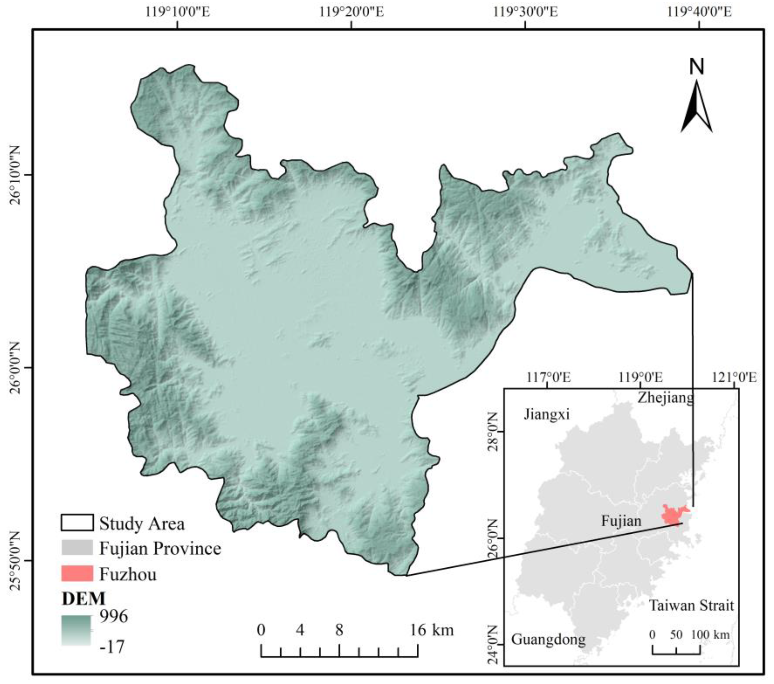
Landsat5 TM and Landsat8 OLI/TIRS images were used to generate the remote sensing ecological index (RSEI) for a total of five periods of 30 m resolution in 2000, 2005, 2010, 2015, and 2020 using the GEE platform. Then, using transfer matrix and spatial autocorrelation techniques, the spatial and temporal change process of ecological environmental quality in Fuzhou’s major metropolitan area was evaluated based on RSEI calculation findings from 2000 to 2020. Finally, the driving power of each element with respect to RSEI changes was investigated using Geodetector, and the varying roles of each factor in space and time were further investigated with respect to the RSEI in combination with geographically weighted regression models.

2.1. Study Area

Fuzhou, the capital of Fujian Province, is located in the eastern portion of China between 25°15′–26°39′ north latitude and 118°08′–120°31′ east longitude in the downstream and coastal area of the Min River (Figure 1). The central city area covers approximately 1447 km², and its landform belongs to a typical estuarine basin, with a relatively flat topography in the main city surrounded by Lianhua Mountain, Gu Mountain, Qi Mountain, and Wuhu Mountain. The study area has a typical subtropical monsoon climate with an average annual precipitation of 900–2100 mm and an average annual temperature of 20–25 °C. The central city of Fuzhou is the most densely populated area in Fujian Province and one of the most economically developed areas. Therefore, it is important to explore the changes in the spatial and temporal patterns of ecological environment quality in the area and to investigate the driving factors affecting the changes to enhance the sustainable development of the city.

2.2. Data Sources and Pre-Processing

In this study, the Google Earth Engine (GEE) platform was used to acquire and process Landsat/TM/OLI/TIRS imagery provided by the United States Geological Survey (USGS) (https://www.usgs.gov, accessed on 17 August 2022). The spatial resolution of the data was 30 m. This data product was processed and acquired on the GEE platform without downloading [24]. In order to accurately assess the ecological environment quality of the study area, 15, 10, 11, 17, and 17 images were used in this study as the base data to construct the RSEI in the above dataset covering the period from April to October, when vegetation growth is at its maximum, and from 2000 to 2020 for five periods (see Appendix A

Table A1. Landsat image series data of Fuzhou from 2000 to 2020.

Year	Sensors	Path/Row	Acquisition Date
2000	Landsat TM	118,042 119,042	19 April 2000; 5 May 2000; 6 June 2000; 8 July 2000; 24 July 2000; 9 August 2000; 10 September 2000; 26 September 2000; 12 May 2000; 13 June 2000; 29 June 2000; 15 July 2000; 31 July 2000; 1 September 2000; 17 September 2000
2005	Landsat TM		4 June 2005; 6 July 2005; 23 August 2005; 8 September 2005; 8 April 2005; 11 June 2005; 27 June 2005; 13 July 2005; 29 July 2005; 30 August 2005
2010	Landsat TM		1 May 2010; 17 May 2010; 4 July 2010; 20 July 2010; 5 August 2010; 21 August 2010; 22 September 2010; 24 May 2010; 11 July 2010; 13 September 2010; 12 August 2010
2015	Landsat OLI		13 April 2015; 29 April 2015; 15 May 2015; 16 June 2015; 2 July 2015; 18 July 2015; 3 August 2015; 19 August 2015; 4 September 2015; 4 April 2015; 7 June 2015; 23 June 2015; 25 July 2015; 26 August 2015; 11 September 2015; 27 September; 9 July 2015
2020	Landsat OLI		10 April 2020; 26 April 2020; 13 June 2020; 29 June 2020; 15 July 2020; 16 August 2020; 1 September 2020; 17 September 2020; 1 April 2020; 17 April 2020; 3 May 2020; 19 May 2020; 20 June 2020; 6 July 2020; 22 July 2020; 7 August 2020; 23 August 2020

for details). We used the median method to synthesize and remove clouds from the images for the five studied periods (see Appendix A for the acquisition dates of the images for each period). Radiometric correction, atmospheric correction, and geometric accuracy correction were performed on the Landsat series surface reflectance data on the GEE platform through a Python script API [25,40]. To avoid the influence of large water areas on the RSEI calculation, the normalized difference water index (MNDWI) [41] was used to mask the water bodies in the study area. Other data are shown in

Table 1. Data sources.

Data Type	Data Format	Resolution	Source
2000–2020 remote sensing images	.tif	30 m	(https://www.usgs.gov) (accessed on 17 August 2022)
Center boundary, government points, park surface, water surface vector data	.shp		(http://zygh.fuzhou.gov.cn) (accessed on 17 August 2022)
DEM	.tif	12.5 m	(https://asf.alaska.edu/) (accessed on 17 August 2022)
Population density (2000~2020)	.tif	100 m	(https://www.worldpop.org/) (accessed on 17 August 2022)
GDP (2000~2020)	.tif	1000 m	(https://www.resdc.cn/) (accessed on 17 August 2022)
Average annual precipitation (2000~2020)	.tif	1000 m	(http://www.geodata.cn/) (accessed on 17 August 2022)

.

2.3. Methods

2.3.1. RSEI Index Calculation

The remote sensing ecological index (RSEI) [18] was employed in this study to monitor changes in ecological conditions in Fuzhou’s center city from 2000 to 2020. Greenness, humidity, heat, and dryness are the four indicators included in the RSEI. The index is calculated according to the following formula:

$$RSEI=f\left(Greenness,Wetness,Heat,Dryness\right)$$

(1)

Greenness represents the normalized difference vegetation index (NDVI); Wetness represents the land surface moisture (WET); Heat represents the land surface temperature (LST); and Dryness represents the normalized differential build-up and bare soil index (NDBSI), which is a combination of the building index (IBI) and soil index (SI). The formulae for the above indices are shown in

Table 2. NDVI, WET, LST, and NDBSI calculation formulae and explanations.

Indicator	Calculation Method	Explanation
NDVI	$\mathrm{NDVI}=\left({\rho }_{\mathit{NIR}}-{\rho }_{\mathit{R}}\right)/\left({\rho }_{\mathit{NIR}}{+\rho }_{\mathit{R}}\right)$	${\rho }_{\mathit{NIR}}$ and ${\rho }_{\mathit{R}}$ for the near-infrared band and the red band, respectively [7,8,42].
WET	${\mathrm{WET}}_{\mathrm{TM}}=0{.0315\rho }_{\mathit{B}}+0{.2021\rho }_{\mathit{G}}+0{.3102\rho }_{\mathit{R}}+0{.1594\rho }_{\mathit{NIR}}-0{.6806\rho }_{\mathit{SWIR}1}-0{.6109\rho }_{\mathit{SWIR}2}$ ${\mathrm{WET}}_{\mathit{OLI}}=0{.1511\rho }_{\mathit{B}}+0{.1972\rho }_{\mathit{G}}+0{.3283\rho }_{\mathit{R}}+0{.3407\rho }_{\mathit{NIR}}-0{.7117\rho }_{\mathit{SWIR}1}-0{.4559\rho }_{\mathit{SWIR}2}$	${\rho }_{\mathit{B}}$, ${\rho }_{\mathit{G}}$, ${\rho }_{\mathit{R}}$, ${\rho }_{\mathit{NIR}}$, ${\rho }_{\mathit{SWIR}1}$, and ${\rho }_{\mathit{SWIR}2}$ correspond to the reflectance of TM and OLI remote sensing images in the blue, green, red, near-infrared, short-wave infrared 1, and short-wave infrared 2 bands, respectively [43,44].
LST	$L_6=\mathit{gain}\times \mathit{DN}+\mathit{bias}$ $T_b{=K}_2/{\mathit{ln}(K}_1/{\mathit{L}}_6+1)$ $LS{T}_{TM}=T_b/\left[1+\left(\lambda T_b/\alpha \right){\ln \epsilon }_6\right]$ $L_{10}={\tau }_{10}\left[{\epsilon }_{10}{B}_{10}\left(T_s\right)+\left(1-{\epsilon }_{10}\right)I_{10}^{\downarrow }\right]+I_{10}^{\uparrow }$ $B_{10}\left(T_s\right)=\left[L_{10}-I_{10}^{\uparrow }-{\tau }_{10}\left(1-{\epsilon }_{10}\right)I_{10}^{\downarrow }\right]/{\tau }_{10}{\epsilon }_{10}$ $LS{T}_{OLI}=K_2/\ln \left(\frac{K_1}{B_{10}\left(T_s\right)}+1\right)$	$\mathrm{Gain}$ and $\mathrm{bias}$ are the transmittance of the atmosphere in the thermal infrared band, the central wavelength ($\mathsf{\lambda }$) is $11.48 \mathsf{\mu }\mathrm{m}$, $\alpha$ is 1.438 × 10−2 mK, ${\epsilon }_6$ is the surface emissivity of band 6, and $K_1$ and $K_2$ are the scaling coefficients obtained in the metadata of the image. ${\tau }_{10}$ is the transmittance of the atmosphere in the thermal infrared band; ${\epsilon }_{10}$ is the surface emissivity of band 10; $B_{10}\left(T_s\right)$ is the thermal radiation brightness of a blackbody at the same temperature as $T_s$; $I_{10}^{\uparrow }$ and $I_{10}^{\downarrow }$ are the upward and downward radiance of the atmosphere, respectively; and $K_1$ and $K_2$ are the scaling coefficients obtained in the metadata of the image [45,46].
NDBSI	$\begin{array}{c}{\mathit{IBI}=\{2\rho }_{\mathit{SWIR}1}{/(\rho }_{\mathit{SWIR}1}{+\rho }_{\mathit{NIR}}{)-[\rho }_{\mathit{NIR}}{/(\rho }_{\mathit{NIR}}{+\rho }_R)+ {\rho }_G{/(\rho }_G+\hfill \\ {\rho }_{\mathit{SWIR}1}{\left)\right]\}/\{2\rho }_{\mathit{SWIR}1}{/(\rho }_{\mathit{SWIR}1}{+\rho }_{\mathit{NIR}}{)+[\rho }_{\mathit{NIR}}{/(\rho }_{\mathit{NIR}}{+\rho }_R{)+\rho }_G{/(\rho }_G{+\rho }_{\mathit{SWIR}1}\left)\right]\}\hfill \end{array}$ $\mathit{SI}=\frac{\left[\left({\rho }_{\mathit{SWIR}1}{+\rho }_R\right)-\left({\rho }_B{+\rho }_{\mathit{NIR}}\right)\right]}{\left[\left({\rho }_{\mathit{SWIR}1}{+\rho }_R\right)+\left({\rho }_B{+\rho }_{\mathit{NIR}}\right)\right]}$ $\mathrm{NDBSI}=(\mathit{IBI}+\mathit{SI})/2$	IBI is the index-based build-up index, SI is the soil index, and the other bands are interpreted as above [19].

.

Because the scale of the above formula is not uniform, a direct PCA calculation would lead to an imbalance in the weights of each indicator. Therefore, the scale must be normalized first according to the following formula:

$$N{I}_i=\frac{I_i-I_{min}}{I_{max}-I_e}$$

(2)

where $N{I}_i$ is the value of a metric after regularization, $I_i$ is the value of the indicator in pixel i, $I_{max}$ is the maximum value of this indicator, and $I_{min}$ is the minimum value of the indicator.

The above four indicators were linked using principal component analysis (PCA), and the first principal component (PCA1) was used to calculate the RSEI because it typically explains more than 80% of the total variation in the dataset and avoids bias in the results due to subjective weighting during calculation (see

Table 3. Results of RSEI principal component analysis.

Year	Index	PC1	PC2	PC3	PC4
2000	NDVI	0.5298	0.5334	−0.4415	0.4897
	WET	0.4230	−0.8151	−0.0404	0.3937
	LST	−0.4464	−0.2178	−0.8658	−0.0604
	NDBSI	−0.5840	0.0601	0.2320	0.7756
	Eigenvalue	0.2150	0.0514	0.0448	0.0034
	Percent eigenvalue	68.34%	16.33%	14.25%	1.08%
2005	NDVI	0.5476	0.4815	0.3973	0.5571
	WET	0.3742	−0.8343	−0.0651	0.3997
	LST	−0.5030	−0.2365	0.8238	0.1114
	NDBSI	−0.5541	0.1272	−0.3991	0.7194
	Eigenvalue	0.2717	0.0413	0.0114	0.0028
	Percent eigenvalue	83.05%	12.63%	3.47%	0.84%
2010	NDVI	0.5582	0.4782	0.3642	0.5719
	WET	0.3857	−0.8545	−0.0153	0.3477
	LST	−0.4965	−0.1934	0.8387	0.1123
	NDBSI	−0.5414	0.0617	−0.4046	0.7344
	Eigenvalue	0.3022	0.0350	0.0116	0.0023
	Percent eigenvalue	86.06%	9.98%	3.32%	0.65%
2015	NDVI	0.5822	0.4325	0.4478	0.5230
	WET	0.3525	−0.8013	−0.1988	0.4405
	LST	−0.4830	−0.3368	0.7971	0.1338
	NDBSI	−0.5509	0.2396	−0.3530	0.7173
	Eigenvalue	0.2455	0.0178	0.0067	0.0011
	Percent eigenvalue	90.58%	6.56%	2.46%	0.40%
2020	NDVI	0.5778	0.4157	0.4792	0.5136
	WET	0.3811	−0.7904	−0.2267	0.4226
	LST	−0.4609	−0.3941	0.7886	0.1016
	NDBSI	−0.5555	0.2170	−0.3115	0.7398
	Eigenvalue	0.2506	0.0178	0.0079	0.0009
	Percent eigenvalue	90.40%	6.41%	2.85%	0.34%

for details).

Similarly, to facilitate metrics and comparisons among indicators, the RSEI₀ can be normalized:

$$RSE{I}_0=1-PC1\left[f\left(NDVI,Wet,LST,NDBSI\right)\right]$$

(3)

$$RSEI=\frac{\left(RSE{I}_0-RSE{I}_{0min}\right)}{\left(RSE{I}_{0max}-RSE{I}_{0min}\right)}$$

(4)

where PC1 is the first principal component of the four indicators. The value of RSEI ranges between [0, 1], and the closer its value is to 1, the better the ecological environment quality. With reference to the grading approach employed by Xu and other scholars [18,19], the RSEI results were classified into five levels: poor (0–0.2), fair (0.2–0.4), moderate (0.4–0.6), good (0.6–0.8), and excellent (0.8–1.0).

2.3.2. Spatial Autocorrelation Analysis

Spatial autocorrelation is an essential indication used to determine whether an element is connected with its neighbors [47,48]. The geographical homogeneous distribution of ecological environmental quality in the research region can be described using spatial autocorrelation analysis of ecological environmental quality [49]. Global spatial autocorrelation (global Moran’s I) and local spatial autocorrelation (local Moran’s I) were utilized in this work to investigate the geographic correlation of RSEI scores.

Global Moran’s I is used to measure the interrelationship of spatial elements, with values in the range of [–1, 1], with larger absolute values indicating greater spatial autocorrelation [50].

$$I=\frac{n}{S_0}\frac{{\sum }_{i=1}^n{\sum }_{j=1}^{n}W\left(i,j\right)\left(X_i-\overline{X}\right)\left(X_j-\overline{X}\right)}{{\sum }_{i=1}^n{\left(X_i-\overline{X}\right)}_i^2}$$

(5)

$$S_0={{\displaystyle \sum }}_{i=1}^n{{\displaystyle \sum }}_{j=1}^{n}W\left(i,j\right)$$

(6)

where n denotes the number of study objects, $X_i$ is the observed value, and $\overline{X}$ is the mean value of $X_i$. $S_0$ is the sum of all weights, and $W\left(i,j\right)$ is the spatial connection matrix between study objects $i,j$.

The results of Moran’s I were tested for significance with the following equation.

$$Z\left(I\right)=\frac{1-E\left(I\right)}{\sqrt{var\left(I\right)}}$$

(7)

where E(I) = (−1)/((n − 1)); var(I) is the variance of I, and |Z(I)| > 1.96 indicates significant spatial autocorrelation. When −1.96 < Z(I) < 1.96, the spatial autocorrelation is not significant.

Local Moran’s I is a decomposition of Moran’s I into individual regional units, i.e., local indicators of spatial association (LISA) [51]. The LISA clustering map has five types of local spatial aggregation: high–high (HH), low–low (LL), low–high (LH), high–low (HL), and insignificant. For a given spatial unit (i):

$$I_i=\frac{X_i-\overline{X}}{S_3}{{\displaystyle \sum }}_{j=1}^{n}W\left(i,j\right)\left(X_j-\overline{X}\right)$$

(8)

$$S_3=\frac{\left({\sum }_{j=1,j\ne i}^n{X}_j^2\right)}{\left(n-1\right)-\overline{X^2}}$$

(9)

where n, $X_i$, and $\overline{X}$ $W\left(i,j\right)$ have the same meaning as in Equation (5).

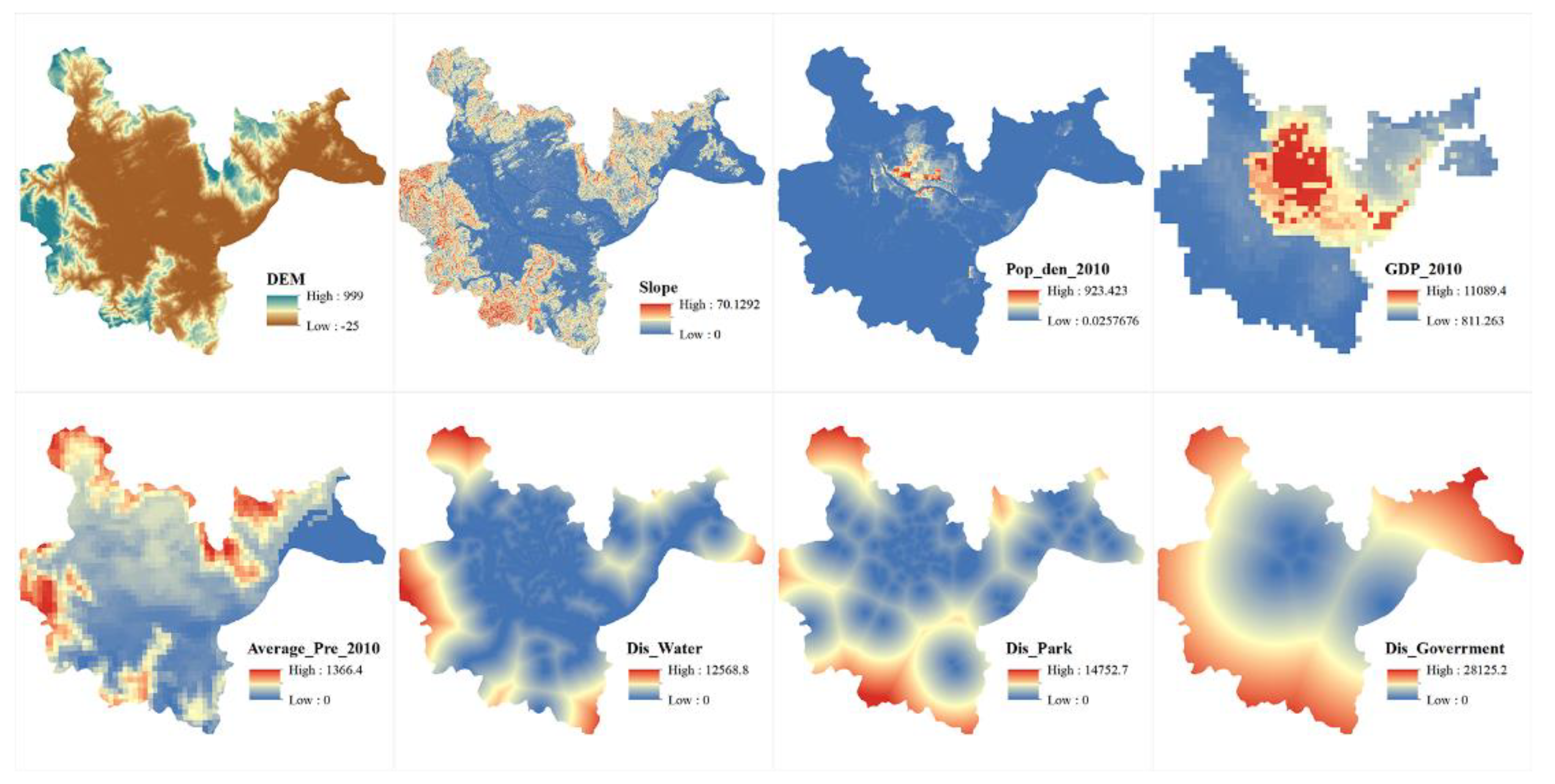
2.3.3. Driver Selection

RSEI alterations are influenced by complex and diverse environmental elements, as well as human activities [52]. The RSEI index from 2000 to 2020 was chosen as the dependent variable in this study, and the representative and easily accessible elevation (X1), slope (X2), population density (X3), GDP (X4), average annual precipitation (X5), distance to water bodies (X6), distance to parks (X7), and distance to government (X8) were chosen as the independent variables. A total of eight variables were employed as drivers (Figure A1). Elevation, slope, and precipitation are important environmental conditions with respect to vegetation growth [7], whereas GDP, population density, and distance from government can reflect the scope and size of human activities [53]. Furthermore, Fuzhou’s central city is a coastal garden city along the river, and water bodies and parks, as urban blue–green spaces, play a positive role in improving the urban ecological environment [54,55].

Geodetector

Geodetector is a spatial statistical method that is used to analyze geographic heterogeneity and to quantify the impact of drivers [29,30,31]. There are a total of four detecting aspects: the factor detector, ecological detector, risk detector, and interaction detector. In this investigation, two detection methods were chosen: the factor detector and interaction detector.

The factor detector is used to detect the spatial heterogeneity of the RSEI and to detect how much of the spatial heterogeneity of the RSEI is explained by a given factor (X). The q-value metric is used with the following equation.

$$q=1-\frac{{\sum }_{h=1}^L{N}_h{\sigma }_h^2}{N{\sigma }^2}=1-\frac{SSW}{SST}$$

(10)

$$SSW={{\displaystyle \sum }}_{h=1}^L{N}_h{\sigma }_h^2 ,SST=N{\sigma }^2$$

(11)

where h = 1, …, L is the stratification or partitioning of variable Y or factor X; $N_h$ and N are the number of cells in a stratum (h) and the whole region, respectively; and ${\sigma }_h^2$ and ${\sigma }^2$ are the variance of Y values in the stratum (h) and the whole region, respectively. SSW and SST are the sum of variance within the stratum and the total variance in the whole region, respectively. q takes values in the range of 0–1, and the larger the value of q, the stronger the explanatory power of factor X with respect to Y [29].

The interaction detector is used to assess whether two factors acting together increase or decrease the explanatory power of the dependent variable (Y) or whether the effects of these factors on Y are independent of each other. First, the q-values of the two factors $X_1$ and $X_2$ are calculated ($q{X}_1$ and $q{X}_2$); then, the q-value of the interaction is calculated, which is a new layer formed by the tangents of the superimposed variables,$X_1$, $X_2$ (q(X₁∩X₂)), and compared with $q{X}_1$,$q{X}_2$. The relationship between two factors can be classified as nonlinearly diminished, one-factor nonlinearly diminished, two-factor enhanced, independent, or nonlinearly enhanced.

Geographically Weighted Regression

Ordinary least squares (OLS) models are commonly used to analyze various regions with similar impacts. However, such interactions are expected to be constant across spatial regions. On the other hand, geographically weighted regression, a local regression model, captures the geographic correlations between the dependent and independent variables that change between locations [56,57,58] and is calculated according to the following equation:

$$Y_i={\beta }_0\left(u_i,v_i\right)+{{\displaystyle \sum }}_k{\beta }_k\left(u_i,v_i\right)X_{ik}+{\epsilon }_i$$

(12)

where $Y_i$ is the dependent variable, $X_{ik}$ is the $k$ independent variables, $\left(u_i,v_i\right)$ is the geographic coordinates of the ith point, ${\beta }_0\left(u_i,v_i\right)$ is the intercept of the ith point, ${\beta }_k\left(u_i,v_i\right)$ is the coefficient of $X_{ik}$, and ${\epsilon }_i$ is the residual of the $i$th point.

A regression equation was generated for each point using weighted least squares, taking only close observations into account. A distance function from the regression point was used to weight each neighboring observation. Fixed Gaussian and adaptive bisquared kernel functions are two common spatial weighting and distance decay methods, respectively. The fixed Gaussian function is denoted as:

$$W_{ij}=\exp \left(-{\left(\frac{d_{ij}}{b}\right)}^2\right)$$

(13)

where $W_{ij}$ is the weight value of observation $j$ for estimation of observation coefficient I, $d_{ij}$ is the distance between $i$ and $j$, and $b$ is the kernel bandwidth.

The adaptive double square function allows the spatial extent to vary at different regression points and includes the same number of adjacent cells for local model estimation. The formula is as follows:

$$W_{ij}=\{\begin{array}{c}{\left(1-d_{ij}^2/b_{i\left(k\right)}^2\right)}^{2}if d_{ij}<b_{i\left(k\right)}\\ 0 if d_{ij}>b_{i\left(k\right)}\end{array}$$

(14)

where $b_{i\left(k\right)}$ is the adaptive bandwidth, and the remaining variables have the same definitions as in Equation (13).

3. Results

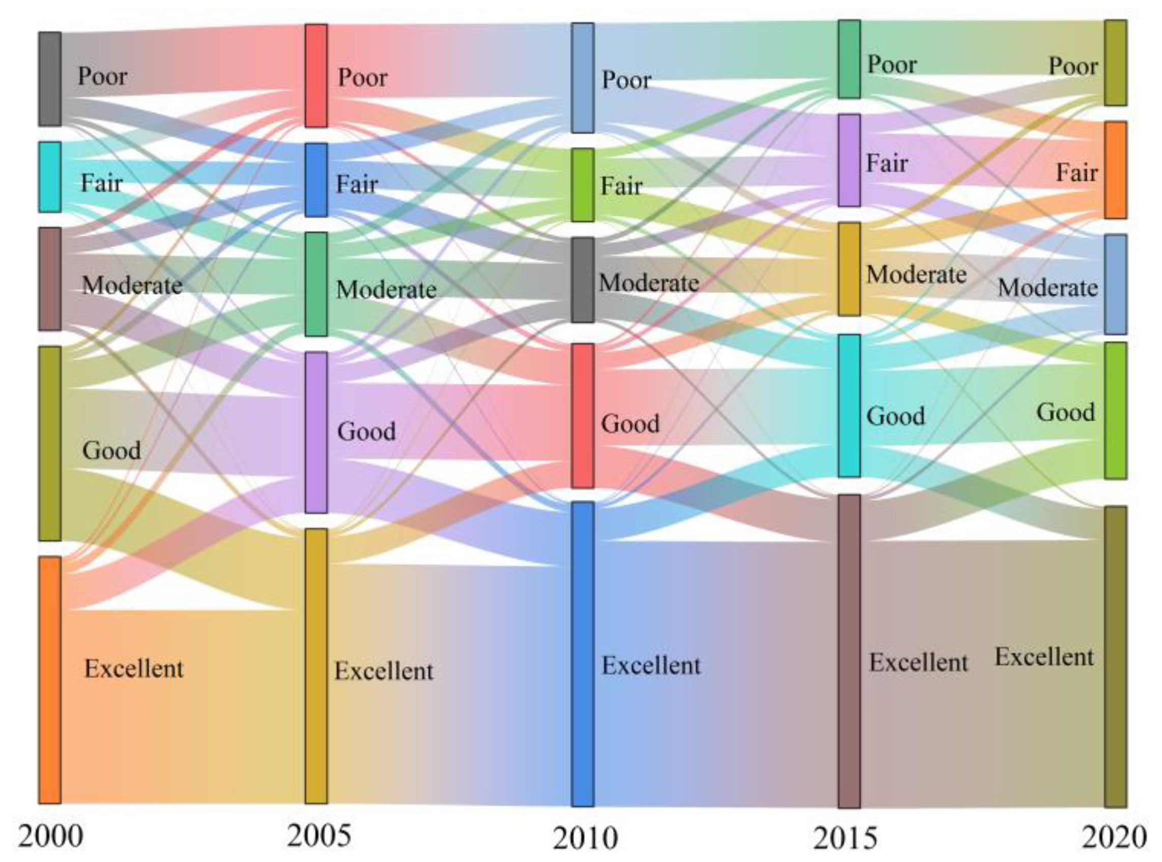
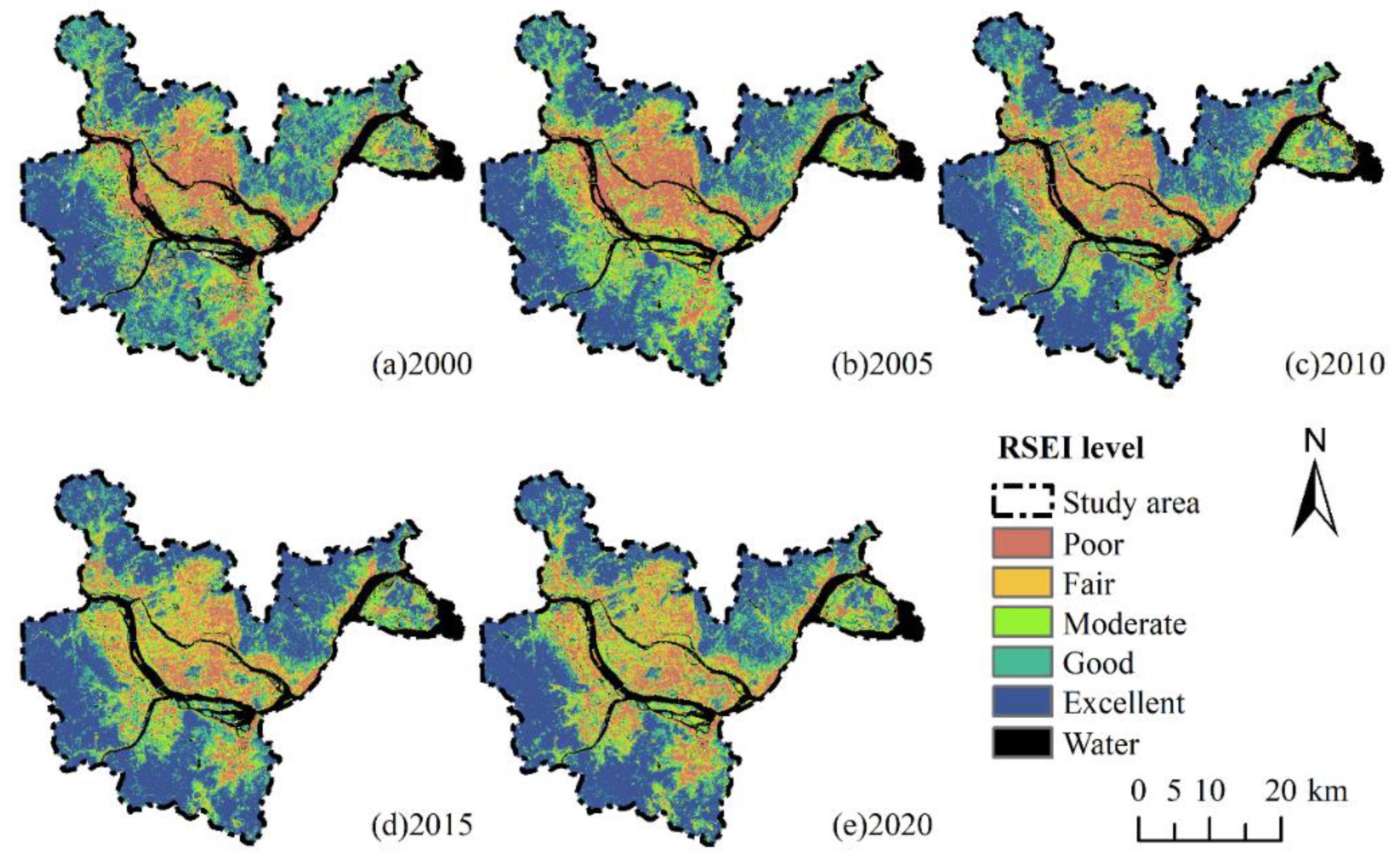
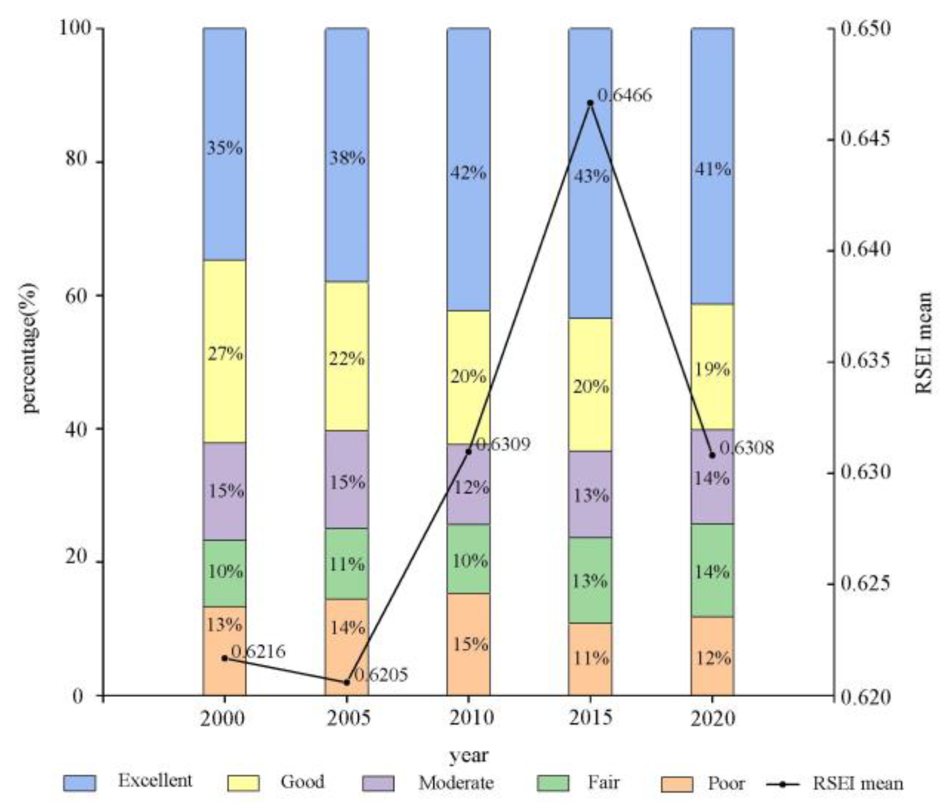
3.1. Results of Ecological Environment Evaluation Based on RSEI

As shown in Table 3, the first principal component (PC1) contributed 68.34%, 83.05%, 86.06%, 90.58%, and 90.40% for the five images from 2000 to 2020, respectively. The results show that PC1 concentrates the majority of the four indicator features, with LST and NDBSI acting as negative indicators and NDVI and WET acting as positive indicators.

Figure 2 depicts the spatial and temporal distribution of RSEI in Fuzhou’s central urban region, with the color ranging from red to blue, representing the change in RSEI from poor to excellent. Overall, the ecological environmental quality of Fuzhou City’s central urban region from 2000 to 2020 is low in the main urban area and excellent in the suburban area, primarily owing to the main urban area’s low height, high level of development, and frequent human activity. The suburban regions of Wuhu Mountain, Gu Mountain, Qi Mountain, and Lianhua Mountain are higher in elevation, with more vegetation and fewer human activities.

Figure 3 depicts the area share of ecological environmental quality in Fuzhou’s city center from 2000 to 2020. Over the last 20 years, the overall proportion of excellent and poor RSEI in Fuzhou has increased, the overall proportion of good and fair has declined, and the proportion of moderate has changed slightly. The mean RSEI value demonstrated a sequence of first increasing and then decreasing. The mean value of RSEI fell somewhat from 2000 to 2005 then rose dramatically in the following decade before falling again between 2015 and 2020. The total ecological quality of Fuzhou City increased gradually over the 20 years but marginally dropped in 2020, demonstrating a bifurcation phenomenon.

Figure 4 shows the statistics of transfers under each level of RSEI in Fuzhou from 2000 to 2020. In addition to the transfer to themselves, poor areas transfer to each other with average areas, medium areas transfer to each other with average and good areas, and good areas transfer to each other with excellent areas. A total of 169.75 km² was transferred out from poor areas during the period of 2000–2020, of which 56.83 km² was transferred to fair areas, accounting for about 33.47% of the total transferred out. A total of 128.07 km² was transferred out of fair areas, of which 34.34 km² was transferred to medium areas, accounting for 26.81% of the total transferred out. The medium area was transferred to all grades, with the most area transferred to excellent areas, accounting for 28.21%.

3.2. Spatial Autocorrelation Analysis of RSEI at Multiple Scales

3.2.1. Global Spatial Autocorrelation

The fishing net tool in ArcGIS was used to generate grids under a total of five scales—300 × 300, 450 × 450, 600 × 600, 750 × 750, and 900 × 900—to ensure the completeness and accuracy of information within the scales, and the 2000–2020 RSEI values were sampled into each grid scale to calculate the Moran index.

Moran’s I is calculated at each scale from 2000 to 2020 in

Table 4. RSEI Moran index at different scales.

	2000			2005			2010			2015			2020
Scale	Moran’s I	z	p	Moran’s I	z	p	Moran’s I	z	p	Moran’s I	z	p	Moran’s I	z	p
300	0.836	154.56	0.000	0.867	215.78	0.000	0.862	158.87	0.000	0.853	207.45	0.001	0.852	157.01	0.000
450	0.816	101.12	0.000	0.848	142.91	0.001	0.845	104.36	0.000	0.833	146.78	0.001	0.830	102.69	0.000
600	0.819	76.32	0.000	0.848	110.71	0.001	0.845	78.40	0.000	0.837	108.73	0.001	0.832	76.98	0.000
750	0.801	60.19	0.000	0.827	87.47	0.001	0.829	62.017	0.000	0.818	86.92	0.001	0.815	60.80	0.000
900	0.803	50.42	0.000	0.827	72.07	0.001	0.822	51.494	0.000	0.811	71.44	0.001	0.803	49.99	0.000

, with all z values exceeding 1.96, suggesting strong spatial autocorrelation of the RSEI in the research area. On the same scale, Moran’s I showed an increasing tendency from 2000 to 2010 and a gradually decreasing trend from 2010 to 2020. Generally, Moran’s I in 2020 is higher than in 2000, indicating that the spatial aggregation effect of the RSEI in Fuzhou City has been intensified, showing a bifurcation phenomenon. As the scale increases, the Moran index appears to decrease, and the z value begins to fall, indicating that as the sampling grid increases, the homogenization between grids increases, and when the grid becomes too large, information within the grid is lost, and the RSEI is no longer spatially self-relevant.

3.2.2. Local Spatial Autocorrelation

LISA clustering maps were created utilizing local spatial autocorrelation to better understand the spatial and temporal distribution of RSEI in Fuzhou’s city center at various scales (Figure 5). At the same scale, the area of insignificant areas reduces with the passage of time, whereas the size of low–low and high–high clustering areas grows. The insignificant areas are primarily located in the suburbs, such as Luangqi Island, whereas the low–low clustering regions are primarily located in the main urban area and along the river, where human activities are more frequent, eventually encroaching on the insignificant areas in the suburbs. The high–high clustering areas are mainly located in the central urban area at the boundary of Qi Mountain, Gu Mountain, Lianhua Mountain, and Wuhu Mountain, with a few in the inner urban area of Gaogai Mountain and Qingliang Mountain. With an increase in the grid scale, the loss of information within the grid causes an increase in insignificant areas and a decrease in high–high and low–low clustering areas. This conclusion is consistent with the results presented in Section 3.2.1.

3.3. RSEI Driver Analysis

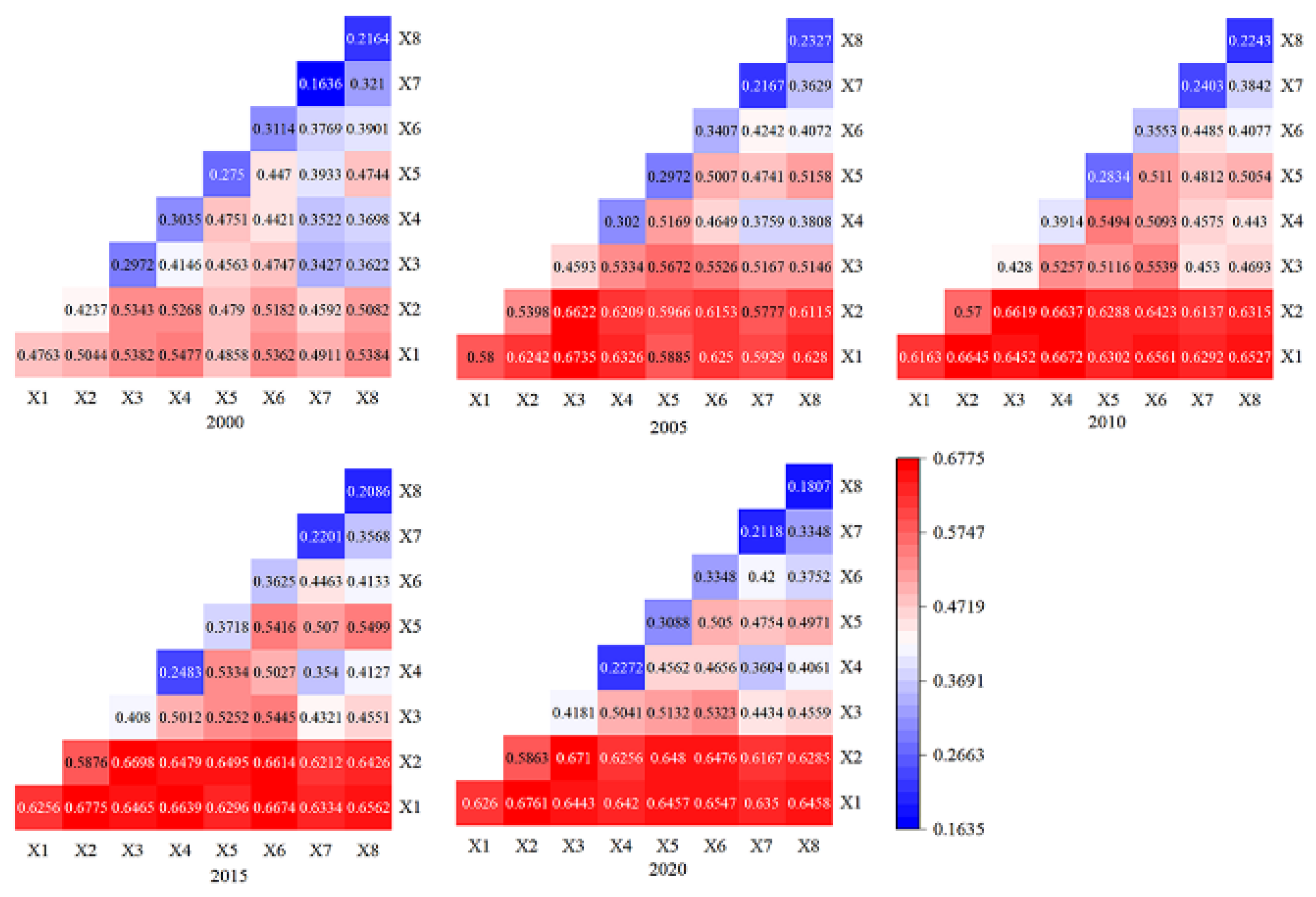
3.3.1. Geodetector-Based Driving Factor Detection

Table 5. Explanatory power of the factors with respect to the RSEI detection for 2000–2020.

	2000		2005		2010		2015		2020
	q	p	q	p	q	p	q	p	q	p
X1	0.48	0.000	0.58	0.000	0.62	0.000	0.63	0.000	0.63	0.000
X2	0.42	0.000	0.54	0.000	0.57	0.000	0.59	0.000	0.59	0.000
X3	0.30	0.000	0.46	0.000	0.43	0.000	0.41	0.000	0.42	0.000
X4	0.30	0.000	0.30	0.000	0.39	0.000	0.25	0.000	0.23	0.000
X5	0.28	0.000	0.30	0.000	0.28	0.000	0.37	0.000	0.31	0.000
X6	0.31	0.000	0.34	0.000	0.36	0.000	0.36	0.000	0.33	0.000
X7	0.16	0.000	0.22	0.000	0.24	0.000	0.22	0.000	0.21	0.000
X8	0.22	0.000	0.23	0.000	0.22	0.000	0.21	0.000	0.18	0.000

demonstrates that all eight factors have a statistically significant effect on RSEI change (p < 0.001). X1 indicates elevation, X2 indicates slope, X3 indicates population density, X4 indicates GDP, X5 indicates average annual precipitation, X6 indicates distance to water bodies, X7 indicates distance to parks, and X8 indicates distance to government. Elevation and slope are the most important elements influencing RSEI variation from 2000 to 2020, and the explanatory power gradually increases with time. With respect to elevation in 2000–2020, the factor’s explanatory power is 0.48, 0.58, 0.62, 0.63, and 0.63 for each of the five surveyed years, respectively, whereas the explanatory power of the slope factor is 0.42, 0.54, 0.57, 0.59, and 0.59, respectively. The main reason is that the degree of development lower in low-elevation and gently sloping areas due to the influence of human activities. The explanatory power of population density increases over time, increasing from 0.3 in 2000 to 0.42 in 2020, demonstrating the environmental impact of human activities, whereas the explanatory power of GDP increased from 0.3 to 0.39 between 2000 and 2010 and decreased from 0.39 to 0.23 between 2010 and 2020, depicting an increasing and then decreasing process. This trend indicates that development and construction are related to environmental protection. Over a 20-year period, the explanatory power of precipitation, which has a facilitating effect on vegetation growth, fluctuates and increases. The explanatory power of the two factors of distance to water bodies and parks appears to fluctuate and increase, indicating that reasonable and effective urban blue–green space planning plays an important role in promoting the urban ecological environment.

Figure 6 depicts the interactions of the factors calculated by the geographic probe; the interactions among the factors are nonlinearly weakly enhanced. The most significant interactions during 2000–2020 are X1∩X4, X1∩X3, X1∩X4, X1∩X2, and X1∩X2, with q values of 0.5477, 0.6735, 0.6672, 0.6775, and 0.6761, respectively. The results indicate that the interaction of elevation with population density and GDP plays a significant role in RSEI in the first decade, whereas the interaction generated by elevation and slope plays the most critical role in the change in RSEI in the second decade. This demonstrates that in the first decade, human activities in low-elevation areas are the main driver of RSEI changes, whereas in the second decade, the low-elevation areas are developed out and the high-elevation areas are mainly protected mountains with positive ecology policies, so the interaction between elevation and slope is obvious.

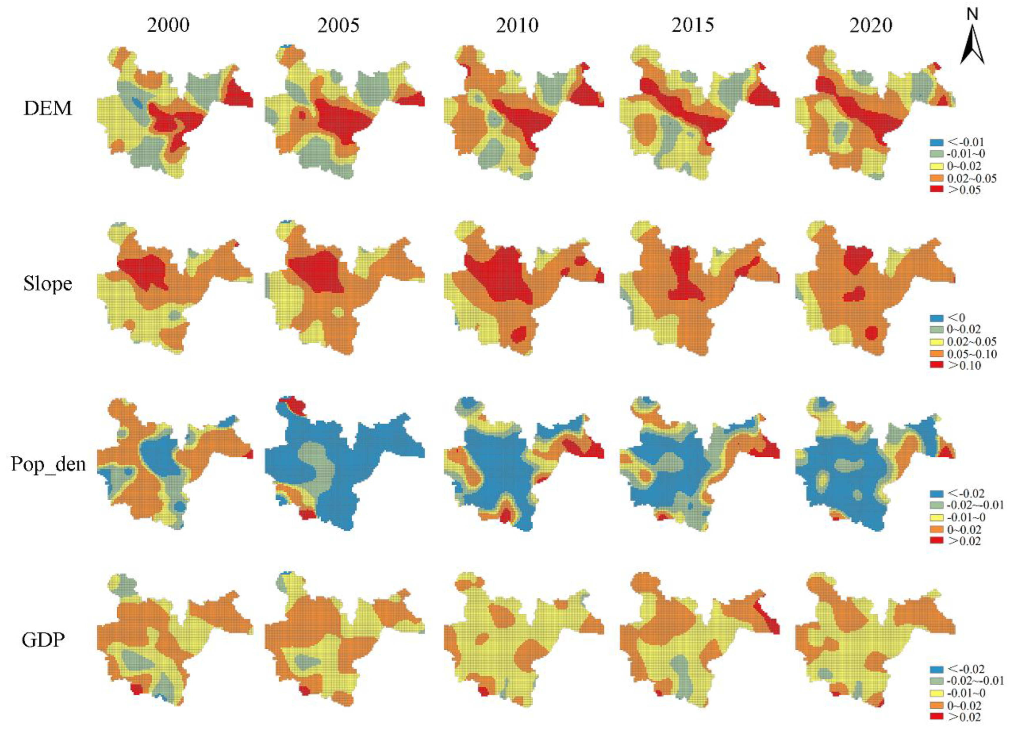
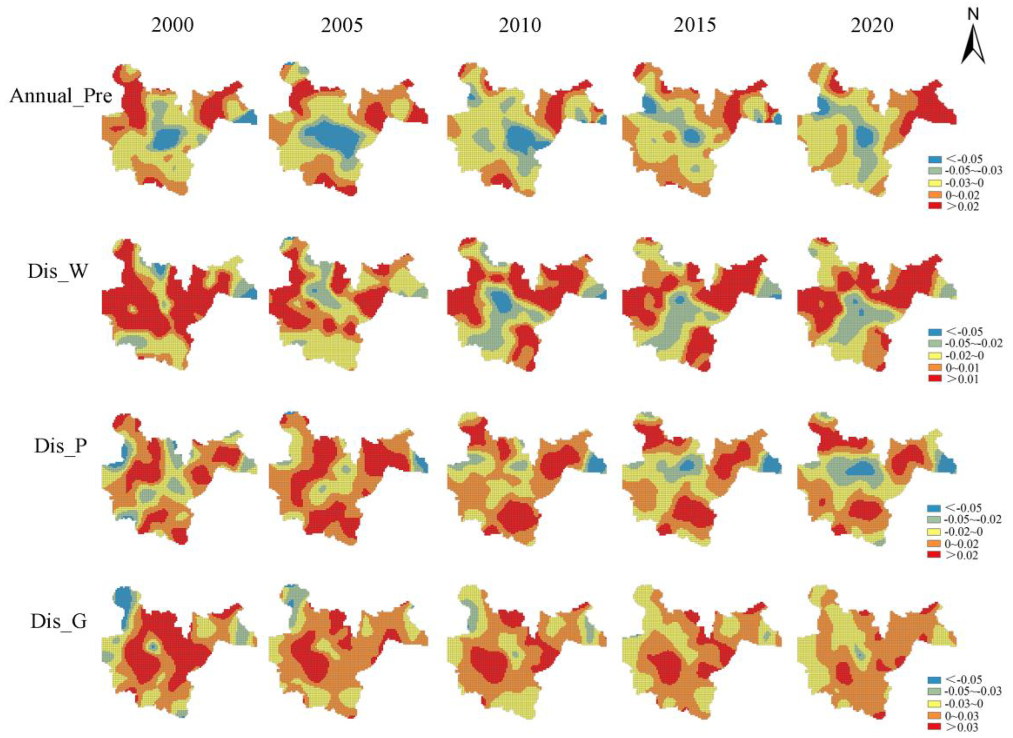
3.3.2. Results of GWR-Based Regression Coefficients of Driving Factors

According to the results presented in Section 3.2, the distribution of RSEI in Fuzhou City is uneven. The geographic detectors could not explain their spatial relationships. To further investigate the spatial influence of each factor on the RSEI in Fuzhou, the local regression coefficients in the GWR model were used to analyze the spatial and temporal differences in the direction and intensity of the effect of the influencing factors.

In the GWR model, each factor needs to meet the requirement of low covariance; the Spearman’s correlation coefficient and variance inflation coefficient between RSEI and each influencing factor were calculated, as shown in

Table 6. Spearman correlation coefficients between RSEI and influencing factors.

	2000			2005			2010			2015			2020
	Coefficient	Sig	VIF	Coefficient	Sig	VIF	Coefficient	Sig	VIF	Coefficient	Sig	VIF	Coefficient	Sig	VIF
X1	0.669 ***	0.000	5.760	0.751 ***	0.000	4.630	0.787 ***	0.000	5.013	0.801 ***	0.000	6.210	0.795 ***	0.000	4.135
X2	0.629 ***	0.000	1.766	0.727 ***	0.000	1.839	0.740 ***	0.000	1.787	0.750 ***	0.000	1.780	0.746 ***	0.000	1.779
X3	−0.469 ***	0.000	2.464	−0.627 ***	0.000	1.469	−0.642 ***	0.000	3.382	−0.645 ***	0.000	3.197	−0.639 ***	0.000	3.267
X4	−0.330 ***	0.000	2.119	−0.334 ***	0.000	2.484	−0.393 ***	0.000	2.806	−0.291 ***	0.000	2.022	−0.256 ***	0.000	1.890
X5	0.508 ***	0.000	4.707	0.533 ***	0.000	3.674	0.512 ***	0.000	3.411	0.621 ***	0.000	4.681	0.529 ***	0.000	2.419
X6	0.529 ***	0.000	2.746	0.562 ***	0.000	2.718	0.582 ***	0.000	2.717	0.607 ***	0.000	2.722	0.594 ***	0.000	2.683
X7	0.395 ***	0.000	2.171	0.466 ***	0.000	1.849	0.496 ***	0.000	2.145	0.484 ***	0.000	2.123	0.466 ***	0.000	2.147
X8	0.374 ***	0.000	2.965	0.411 ***	0.000	3.380	0.426 ***	0.000	3.158	0.433 ***	0.000	3.181	0.413 ***	0.000	2.750

Note: ***, **, and * represent significance at the 0.001, 0.01, and 0.05 level, respectively.

. There were significant correlations between RSEI and each factor (p < 0.001), and the VIF values of each factor were below 7.5, indicating that the degree of covariance among the factors was low. Elevation, slope, average annual rainfall, distance from water bodies, distance from parks, and distance from government are significantly and positively correlated with RSEI; GDP and population density are significantly and negatively correlated with RSEI. The highest correlation coefficients were found between elevation and slope in 2020, followed by GDP and average annual rainfall. The results are consistent with the factor detection (Table 5 and Table 6).

Table 7. Estimated parameters of the GWR model.

Year	Residual Squares	Effective Number	AICc	R2	R2 Adjusted
2000	74.36	99.52	−5084.93	0.76	0.75
2005	56.78	76.41	−6274.63	0.84	0.83
2010	58.80	86.81	−6111.41	0.84	0.84
2015	52.85	85.32	−6571.09	0.83	0.83
2020	48.87	86.01	−6906.42	0.84	0.84

shows the parameters of the GWR model-fitting results, showing that the goodness of fit for each year is greater than 0.75, indicating that the selected factors fit the RSEI well and can explain the local variations affecting the RSEI.

With 600 × 600 m as the sampling grid, the RSEI of each period was used as the dependent variable, and a total of eight factors, namely elevation, slope, population density, GDP, average annual precipitation, distance to water bodies, distance to parks, and distance to government, were used as independent variables, with a fixed Gaussian kernel function; the best bandwidth was selected with the cross-validation (CV) method. The regression coefficients of the elevation, slope, population density, and GDP factors from 2000 to 2020 are plotted in Figure 7. Figure 8 shows the regression coefficients of the factors of annual average rainfall, distance from water bodies, distance from parks, and distance from government from 2000 to 2020.

The DEM, slope, and RSEI are significantly positively correlated with each other, and the regression coefficients in Figure 7 show that DEM and slope positively contribute to the RSEI in most parts of the study area. The main reason for this is that the two areas of the Minjiang River in Fuzhou City have a positive effect on the RSEI, mainly because both sides of the Min River in Fuzhou City are lower in elevation and more developed, and the ecological environment is more sensitive to DEM in this part of the city. The areas that play a negative inhibitory role are mainly concentrated in the south and northeast of the study area, and the area is gradually decreasing, mainly because Fuzhou City has introduced relevant policies and environmental protection measures to suppress indiscriminate logging and protect the surrounding mountains.

The slope factor has a facilitating effect on RSEI in general, which is most obvious in the center of the study area and decreasing sharply after 2010. Urbanization in Fuzhou City accelerated after 2010, with high development intensity and gently sloping areas being constructed as artificial surfaces.

Population density, GDP, and RSEI show an overall negative correlation. Figure 7 shows that the negative suppressive effect of the population density factor is mainly concentrated in the middle of the study area, again showing a trend of increasing first and then decreasing. The negative suppressive effect of the population density factor in Minhou County in the west and south direction of the study area gradually strengthens after 2010, mainly because Fuzhou City started to build a university city after 2010, with a dense population, and as the capital city of Fujian Province, the development within the third ring of the main city is exhausted, with development spreading to the suburban area.

The GDP factor also shows a negative inhibitory effect on RSEI in general, and its inhibitory effect also shows an increasing and then decreasing trend. Before 2010, the inhibitory effect of the GDP factor on RSEI gradually increased and covered almost the whole study area in 2010. After 2010, the inhibitory effect area gradually decreased, which may have been caused by the economic development pattern before 2010 at the expense of the environment. In addition, the change in national and local policies, which resulted in the development a green and low-carbon economic model, led to a decrease in the inhibitory effect of GDP on RSEI areas.

Figure 8 shows the local regression coefficients of the four drivers of average annual precipitation, distance to water bodies, distance to parks, and distance to government for the RSEI.

Generally speaking, precipitation promotes plant growth and improves temperature, with a positive relationship with RSEI. However, the effect of the annual average precipitation factor on RSEI (Figure 8) shows a suppressive effect in the middle spatial area and a promoting effect around the mountain at the boundary of the study area. The area of the promoting effect gradually decreases with time, and the area of the inhibiting effect gradually increases. The reason for the increase in the inhibitory phenomenon may be the large increase in impervious surface during the urbanization process. For example, the Fuzhou South Railway Station, located in the southern part of CangShan District, was put into operation in 2010. Because Fuzhou City belongs to a typical estuarine basin topography, the mountains at the boundary of the study area are at a high elevation, and air rises due to the lifting effect of the topography, continuously cooling and condensing to form precipitation. The result is a strong boost in the border area.

The distance from water bodies, parks, and government is demonstrated by the Spearman results. These three factors are positively correlated with RSEI, implying that the farther from water bodies, parks, and government, the higher the quality of the ecological environment. However, water bodies and parks play a role in improving the environment as blue–green spaces in the city. Urban parks, water bodies, and government sites in Fuzhou are almost all located within the third ring, with high construction density, and are subject to high levels of human interference. Therefore, spatially, the positive contribution of distance from water bodies is mainly distributed in the northeast, west, and south of the study area. This is consistent with the distribution pattern of the RSEI (0.8–1). The areas with negative inhibitory effects are mainly distributed in the third ring of the urban center, indicating that in this area, the factor of distance from water bodies has a negative effect on the RSEI, i.e., the closer to a water body, the better the ecological environment.

The factors of distance from parks and distance factor from water bodies generally appear to coincide. The positive promoting effect gradually migrates to the surroundings in the study area, and the areas with a negative inhibiting effect gradually move closer to the center. This phenomenon shows that parks and water bodies, as urban blue–green spaces, contribute to the ecological quality of the city. However, this effect is not unlimited.

The factor of distance from government positive contributes to the RSEI as a whole. That is, in areas in which government services are located tend to be more intensively built-up; the further away from government, the better the ecological environment.

4. Discussion

4.1. Calculation of RSEI

The greenness (NDVI) and humidity (WET) indicators were found to have a positive effect on the RSEI, whereas the dryness (NDBSI) and heat (LST) indicators had a negative effect on the RSEI. These results are similar to those reported in previous studies [59,60,61]. The effect of the greenness and dryness indicators was more significant than that of other indicators. The ecological environmental quality of waters is also a problem faced by Fuzhou City, although the ecological environmental quality of water and air quality were not adequately studied in this work. The ecological effects of water and air quality should be further incorporated into the ecological environment assessment of Fuzhou City in the future.

In this paper, the weights used to calculate the RSEI for 2000 (PC1) are low, although the results were unaffected. The principal component analysis applied here focuses on the ability to correctly represent the ecological indicators. For example, in Table 3, the loadings of the principal components PC1, NDVI, representing greenness, and WET, representing humidity, have positive values, indicating that they contribute positively to the ecology, whereas the loadings of LST, representing heat, and NDBSI, representing dryness, have negative values, indicating that they contribute negatively to the ecology, as expected. In contrast, in PC2, the WET load values are negative, and NDBSI load values are positive, in contrast to the actual ecological situation. Similarly, in PC3, the NDVI load value, which represents greenness, is negative, whereas in PC4, the NDBSI load value, which has a negative effect on the environment, is the highest, which obviously contradicts the reality of the situation. Therefore, only PC1 can be used for reasonable interpretation of the RSEI and does not affect the results.

4.2. Spatial Distribution Pattern of RSEI

The mean values of the RSEI in Fuzhou from 2000 to 2020 were 0.6216, 0.6205, 0.6309, 0.6466, and 0.6308 for each of the five investigated years, respectively, and the proportion of areas with an excellent rating (0.8–1) increased from 38% to 41%. This is consistent with the results reported by scholars in a previous study [20]. However, the improvement with respect to the mean value is not significant, mainly because the topography of Fuzhou City led to the deterioration of the RSEI in the central area, whereas the mountains in the suburbs are protected by environmental policy, resulting in a gradual increase in the number of areas with good RSEI (Figure 2). This is the main reason why the mean value of the RSEI does not change much. Therefore, it is necessary to study the urban–rural RSEI drivers in a comparative manner in future research.

In addition, the RSEI of Fuzhou is strongly spatially autocorrelated, as manifested by the erosion of low–low clusters and high–high clusters to insignificant areas. Generally speaking, the low–low clustering areas are mainly located in central areas, where human activities are more intensive, and gradually expand to the outskirts of the city with urban development, encroaching on the insignificant areas. The high–high clustering areas, on the other hand, are mainly located among the hills along the city boundaries, which have been protected by ecological red lines in recent years. The focus of future protection should be to strictly limit the scale of construction land in the insignificant areas, in addition to the mountains at the urban boundaries.

4.3. Driving Forces of RSEI

In this study, the positive effects of elevation and slope on the distribution of RSEI gradually increased, indicating that high-altitude areas and steep slopes are more difficult to develop and unsuitable for human life and habitation, resulting in a better ecological environment. This is consistent with the findings reported in related studies [62]. Economic and population development is bound to put pressure on the environment, especially in urban centers. However, with the proposed eco-environmental policy in China, the explanatory power of GDP with respect to the spatial differentiation of RSEI decreased from 2010 onwards, demonstrating that economic growth is no longer achieved at the expense of the environment. In addition, the positive driving effect of two factors, distance to water bodies and distance to parks, increased, suggesting that the active construction of urban blue–green spaces has played a role in improving the urban environment.

In addition to exploring the explanatory power of each driver with respect to the spatial variation of the RSEI, it will be beneficial to explore the scope and effect of each driver in space and time for different regions to develop corresponding policies. In this study, we successfully quantified the range of positive and negative effects of each driver using a geographically weighted regression model. The results show that the range of drivers varies across time. For example, the positive driving effect of the elevation and slope factor gradually shifted to both sides of the Min River and the urban center, indicating that small mountains in the urban center play a key role in improving the ecological environment and should be protected, with restrictions on development. The negative driving effect of the GDP and population density factors gradually expanded to the outskirts of the city, mainly due to the large amount of land resources required for the development and construction of new urban areas in Fuzhou. Therefore, during the construction of new urban areas, attention should be paid to the reasonable protection of local natural environmental resources. With respect to the average annual precipitation factor, we found that it plays a negative role in the central urban areas, mainly due to the large amount of impervious surfaces in these areas, leading to problems such as rainwater runoff. Therefore, an appropriate increase in rain gardens in these areas and strengthening of the construction of sponge cities will help alleviate ecological and environmental problems in central urban areas. In addition, parks and water bodies in cities play a role in improving the ecological environment, so in the process of urbanization, not only should urban construction be planned scientifically and reasonably, but attention should also be paid to adding green areas and water bodies in cities.

5. Conclusions

This study not only provides a rapid and effective method for evaluation of regional ecological environmental quality, but we also explored the driving factors affecting the spatial differentiation of ecological environmental quality through multiple methods. The reported results provide a scientific basis for maintenance of the sustainable development of cities to promote urbanization.

The mean RSEI value in the study showed an increasing trend followed by a decreasing trend. The poor area of RSEI decreased by 17.27 km², the fair area increased by 55.49 km², the moderate area decreased by 1.84 km², the good area decreased by 106.02 km², and the excellent area increased by 97.78 km² during the 20-year study period. The RSEI in all periods was obviously spatially autocorrelated; the low–low clustering area is mainly distributed in the central urban area, and the high–high clustering area is mainly distributed in the mountain and high-altitude areas at the boundary of the study area. Elevation, slope, average annual precipitation, distance from water bodies, distance from parks, and distance from government have a positive effect on the spatial differentiation of the RSEI, whereas population density and GDP have a negative effect. The areas with positive driving effects have decreased over time and are mainly concentrated at the boundary of the study area. Areas with a negative driving effect are increasing, gradually spreading to the border areas. The elevation and slope factors are increasingly able to explain the spatial divergence of the RSEI, indicating that the urbanization process of Fuzhou City is continuing, and the low-elevation areas are being exploited artificially. Although the mountains in the high-elevation suburbs can be protected, the ecological and environmental problems in the urban center areas are still serious. Therefore, we suggest building more urban parks in the central areas of the city to improve the quality of the ecological environment and to develop land resources rationally during future development to protect the local natural environmental resources.

References

1. Zhao, S.; Da, L.; Tang, Z.; Fang, H.; Song, K.; Fang, J. Ecological consequences of rapid urban expansion: Shanghai, China. Front. Ecol. Environ. 2006, 4, 341–346. [Google Scholar] [CrossRef]
2. Shen, W.; Wu, J.; Grimm, N.B.; Hope, D. Effects of urbanization-induced environmental changes on ecosystem functioning in the Phoenix metropolitan region, USA. Ecosystems 2008, 11, 138–155. [Google Scholar] [CrossRef]
3. Luo, W.; Bai, H.; Jing, Q.; Liu, T.; Xu, H. Urbanization-induced ecological degradation in Midwestern China: An analysis based on an improved ecological footprint model. Resour. Conserv. Recycl. 2018, 137, 113–125. [Google Scholar] [CrossRef]
4. Rizwan, A.M.; Dennis, L.Y.C.; Chunho, L.I.U. A review on the generation, determination and mitigation of Urban Heat Island. J. Environ. Sci. 2008, 20, 120–128. [Google Scholar] [CrossRef]
5. Liu, W.; Chen, W.; Peng, C. Assessing the effectiveness of green infrastructures on urban flooding reduction: A community scale study. Ecol. Model. 2014, 291, 6–14. [Google Scholar] [CrossRef]
6. Aronson, M.F.J.; Lepczyk, C.A.; Evans, K.L.; Goddard, M.A.; Lerman, S.B.; Maclvor, J.S.; Nilon, C.H.; Vargo, T. Biodiversity in the city: Key challenges for urban green space management. Front. Ecol. Environ. 2017, 15, 189–196. [Google Scholar] [CrossRef]
7. Peng, W.; Kuang, T.; Tao, S. Quantifying influences of natural factors on vegetation NDVI changes based on geographical detector in Sichuan, western China. J. Clean. Prod. 2019, 233, 353–367. [Google Scholar] [CrossRef]
8. Huang, S.; Tang, L.; Hupy, J.P.; Wang, Y.; Shao, G. A commentary review on the use of normalized difference vegetation index (NDVI) in the era of popular remote sensing. J. For. Res. 2021, 32, 1–6. [Google Scholar] [CrossRef]
9. Asner, G.P.; Scurlock, J.M.O.A.; Hicke, J. Global synthesis of leaf area index observations: Implications for ecological and remote sensing studies. Glob. Ecol. Biogeogr. 2003, 12, 191–205. [Google Scholar] [CrossRef]
10. Jiang, Z.; Huete, A.R.; Didan, K.; Miura, T. Development of a two-band enhanced vegetation index without a blue band. Remote Sens. Environ. 2008, 112, 3833–3845. [Google Scholar] [CrossRef]
11. Li, Z.L.; Tang, B.H.; Wu, H.; Ren, H.; Yan, G.; Wan, Z.; Trigo, I.F.; Sobrion, J.A. Satellite-derived land surface temperature: Current status and perspectives. Remote Sens. Environ. 2013, 131, 14–37. [Google Scholar] [CrossRef]
12. Jiang, J.; Tian, G. Analysis of the impact of land use/land cover change on land surface temperature with remote sensing. Procedia Environ. Sci. 2010, 2, 571–575. [Google Scholar] [CrossRef]
13. Du, L.; Song, N.; Liu, K.; Hou, J.; Hu, Y.; Zhu, Y.; Wan, X.; Wang, L.; Guo, Y. Comparison of two simulation methods of the temperature vegetation dryness index (TVDI) for drought monitoring in semi-arid regions of China. Remote Sens. 2017, 9, 177. [Google Scholar] [CrossRef]
14. Rahman, S.; Mesev, V. Change vector analysis, tasseled cap, and NDVI-NDMI for measuring land use/cover changes caused by a sudden short-term severe drought: 2011 Texas event. Remote Sens. 2019, 11, 2217. [Google Scholar] [CrossRef]
15. Yue, A.; Zhang, Z. Analysis and research on ecological situation change based on EI value. Green Sci. Technol. 2018, 14, 182–184. [Google Scholar]
16. Wang, C.; Jiang, Q.; Shao, Y.; Sun, S.; Xiao, L.; Guo, J. Ecological environment assessment based on land use simulation: A case study in the Heihe River Basin. Sci. Total Environ. 2019, 697, 133928. [Google Scholar] [CrossRef]
17. Wu, X.; Zhang, H. Evaluation of ecological environmental quality and factor explanatory power analysis in western Chongqing, China. Ecol. Indic. 2021, 132, 108311. [Google Scholar] [CrossRef]
18. Xu, H.Q. A remote sensing urban ecological index and its application. Acta Ecol. Sin. 2013, 33, 7853–7862. [Google Scholar]
19. Hu, X.; Xu, H. A new remote sensing index for assessing the spatial heterogeneity in urban ecological quality: A case from Fuzhou City, China. Ecol. Indic. 2018, 89, 11–21. [Google Scholar] [CrossRef]
20. Yue, H.; Liu, Y.; Li, Y.; Lu, Y. Eco-Environmental Quality Assessment in China’s 35 Major Cities Based on Remote Sensing Ecological Index. IEEE Access 2019, 7, 51295–51311. [Google Scholar] [CrossRef]
21. Yuan, B.; Fu, L.; Zou, Y.; Zhang, S.; Chen, X.; Li, F.; Deng, Z.; Xie, Y. Spatiotemporal change detection of ecological quality and the associated affecting factors in Dongting Lake Basin, based on RSEI. J. Clean. Prod. 2021, 302, 126995. [Google Scholar] [CrossRef]
22. Xiong, Y.; Xu, W.; Lu, N.; Huang, S.; Wu, C.; Wang, L.; Dai, F.; Kou, W. Assessment of spatial–temporal changes of ecological environment quality based on RSEI and GEE: A case study in Erhai Lake Basin, Yunnan province, China. Ecol. Indic. 2021, 125, 107518. [Google Scholar] [CrossRef]
23. Liu, C.; Yang, M.; Hou, Y.; Zhao, Y.; Xue, X. Spatiotemporal evolution of island ecological quality under different urban densities: A comparative analysis of Xiamen and Kinmen Islands, southeast China. Ecol. Indic. 2021, 124, 107438. [Google Scholar] [CrossRef]
24. Gorelick, N.; Hancher, M.; Dixon, M.; Ilyushchenko, S.; Thau, D.; Moore, R. Google Earth Engine: Planetary-scale geospatial analysis for everyone. Remote Sens. Environ. 2017, 202, 18–27. [Google Scholar] [CrossRef]
25. Kumar, L.; Mutanga, O. Google Earth Engine applications since inception: Usage, trends, and potential. Remote Sens. 2018, 10, 1509. [Google Scholar] [CrossRef]
26. Guo, G.; Wu, Z.; Chen, Y. Evaluation of spatially heterogeneous driving forces of the urban heat environment based on a regression tree model. Sustain. Cities Soc. 2020, 54, 101960. [Google Scholar] [CrossRef]
27. Chen, M.; Luo, Y.; Shen, Y.; Han, Z.; Cui, Y. Driving force analysis of irrigation water consumption using principal component regression analysis. Agric. Water Manag. 2020, 234, 106089. [Google Scholar] [CrossRef]
28. He, Y.X.; Yi, G.H.; Zhang, T.B. The EVI trends and driving factors in Red River Basin affected by the “corridor-corridorbarrier” function during 2000–2014. ACTA Ecol. Sin. 2018, 38, 2056–2064. [Google Scholar]
29. Wu, J.; Li, J.; Peng, J.; Li, W.; Xu, G.; Dong, C. Applying land use regression model to estimate spatial variation of PM2. 5 in Beijing, China. Environ. Sci. Pollut. Res. 2015, 22, 7045–7061. [Google Scholar] [CrossRef]
30. Wang, J.F.; Li, X.H.; Christakos, G.; Lian, Y.L.; Zhang, T.; Gu, X.; Zheng, X.Y. Geographical detectors-based health risk assessment and its application in the neural tube defects study of the Heshun Region, China. Int. J. Geogr. Inf. Sci. 2010, 24, 107–127. [Google Scholar] [CrossRef]
31. Wang, J.F.; Hu, Y. Environmental health risk detection with GeogDetector. Environ. Model. Softw. 2012, 33, 114–115. [Google Scholar] [CrossRef]
32. Wang, J.F.; Zhang, T.L.; Fu, B.J. A measure of spatial stratified heterogeneity. Ecol. Indic. 2016, 67, 250–256. [Google Scholar] [CrossRef]
33. Ju, H.; Zhang, Z.; Zuo, L.; Wang, J.; Zhang, S.; Wang, X.; Zhao, X. Driving forces and their interactions of built-up land expansion based on the geographical detector–a case study of Beijing, China. Int. J. Geogr. Inf. Sci. 2016, 30, 2188–2207. [Google Scholar] [CrossRef]
34. Song, T.; Cheng, Y.; Liu, W.; Liu, H. Spatial difference and mechanisms of influence of geo-economy in the border areas of China. J. Geogr. Sci. 2017, 27, 1463–1480. [Google Scholar] [CrossRef]
35. Zuo, S.; Dai, S.; Song, X.; Xu, C.; Liao, Y.; Chang, W.; Chen, Q.; Li, Y.; Tang, J.; Man, W.; et al. Determining the mechanisms that influence the surface temperature of urban forest canopies by combining remote sensing methods, ground observations, and spatial statistical models. Remote Sens. 2018, 10, 1814. [Google Scholar] [CrossRef]
36. Liang, P.; Yang, X. Landscape spatial patterns in the Maowusu (Mu Us) Sandy Land, northern China and their impact factors. Catena 2016, 145, 321–333. [Google Scholar] [CrossRef]
37. Huang, J.; Wang, J.; Bo, Y.; Xu, C.; Hu, M.; Huang, D. Identification of health risks of hand, foot and mouth disease in China using the geographical detector technique. Int. J. Environ. Res. Public Health 2014, 11, 3407–3423. [Google Scholar] [CrossRef]
38. Sun, K.; Xu, Z.M. The impacts of human driving factors on grey water footprint in China using a GWR model. Chin. J. Geogr. Res. 2016, 35, 37–48. [Google Scholar]
39. Li, S.; Zhao, Z.; Miaomiao, X.; Wang, Y. Investigating spatial non-stationary and scale-dependent relationships between urban surface temperature and environmental factors using geographically weighted regression. Environ. Model. Softw. 2010, 25, 1789–1800. [Google Scholar] [CrossRef]
40. Wang, X.; Xiao, X.; Zou, Z.; Chen, B.; Ma, J.; Dong, J.; Doughty, R.B.; Zhong, Q.; Qin, Y.; Dai, S.; et al. Tracking annual changes of coastal tidal flats in China during 1986–2016 through analyses of Landsat images with Google Earth Engine. Remote Sens. Environ. 2020, 238, 110987. [Google Scholar] [CrossRef]
41. Xu, H. Modification of normalised difference water index (NDWI) to enhance open water features in remotely sensed imagery. Int. J. Remote Sens. 2006, 27, 3025–3033. [Google Scholar] [CrossRef]
42. Kogan, F.; Gitelson, A.; Zakarin, E.; Spivak, L.; Lebed, L. AVHRR-based spectral vegetation index for quantitative assessment of vegetation state and productivity. Photogramm. Eng. Remote Sens. 2003, 69, 899–906. [Google Scholar] [CrossRef]
43. Crist, E.P. A TM tasseled cap equivalent transformation for reflectance factor data. Remote Sens. Environ. 1985, 17, 301–306. [Google Scholar] [CrossRef]
44. Baig, M.H.A.; Zhang, L.; Shuai, T.; Tong, Q. Derivation of a tasselled cap transformation based on Landsat 8 at-satellite reflectance. Remote Sens. Lett. 2014, 5, 423–431. [Google Scholar] [CrossRef]
45. Estoque, R.C.; Murayama, Y.; Myint, S.W. Effects of landscape composition and pattern on land surface temperature: An urban heat island study in the megacities of Southeast Asia. Sci. Total Environ. 2017, 577, 349–359. [Google Scholar] [CrossRef]
46. Jiménez-Muñoz, J.C.; Sobrino, J.A.; Skoković, D.; Mattar, C.; Cristóbal, J. Land surface temperature retrieval methods from Landsat-8 thermal infrared sensor data. IEEE Geosci. Remote Sens. Lett. 2014, 11, 1840–1843. [Google Scholar] [CrossRef]
47. Legendre, P. Spatial autocorrelation: Trouble or new paradigm? Ecology 1993, 74, 1659–1673. [Google Scholar] [CrossRef]
48. Diniz-Filho, J.A.F.; Bini, L.M.; Hawkins, B.A. Spatial autocorrelation and red herrings in geographical ecology. Glob. Ecol. Biogeogr. 2003, 12, 53–64. [Google Scholar] [CrossRef]
49. Boori, M.S.; Choudhary, K.; Paringer, R.; Kupriyanov, A. Spatiotemporal ecological vulnerability analysis with statistical correlation based on satellite remote sensing in Samara, Russia. J. Environ. Manag. 2021, 285, 112138. [Google Scholar] [CrossRef]
50. Cliff, A.D.; Ord, J.K. Spatial Processes: Models & Applications; Taylor & Francis: Abingdon, UK, 1981. [Google Scholar]
51. Anselin, L. Local indicators of spatial association—LISA. Geogr. Anal. 1995, 27, 93–115. [Google Scholar] [CrossRef]
52. Yang, X.; Meng, F.; Fu, P.; Zhang, Y.; Liu, Y. Spatiotemporal change and driving factors of the Eco-Environment quality in the Yangtze River Basin from 2001 to 2019. Ecol. Indic. 2021, 131, 108214. [Google Scholar] [CrossRef]
53. Liu, Y.S.; Li, J.T. Geographic detection and optimizing decision of the differentiation mechanism of rural poverty in China. Acta Geogr. Sin. 2017, 72, 161–173. [Google Scholar]
54. Liu, L.; Jensen, M.B. Green infrastructure for sustainable urban water management: Practices of five forerunner cities. Cities 2018, 74, 126–133. [Google Scholar] [CrossRef]
55. Kazmierczak, A.; Carter, J. Adaptation to Climate Change Using Green and Blue Infrastructure. A Database of Case Studies; University of Manchester: Manchester, UK, 2010. [Google Scholar]
56. Zhao, R.; Zhan, L.; Yao, M.; Yang, L. A geographically weighted regression model augmented by Geodetector analysis and principal component analysis for the spatial distribution of PM2.5. Sustain. Cities Soc. 2020, 56, 102106. [Google Scholar] [CrossRef]
57. Wu, X.; Yin, J.; Li, C.; Xiang, H.; Lv, M.; Guo, Z. Natural and human environment interactively drive spread pattern of COVID-19: A city-level modeling study in China. Sci. Total Environ. 2021, 756, 143343. [Google Scholar] [CrossRef]
58. Fotheringham, A.S.; Brunsdon, C.; Charlton, M. Geographically Weighted Regression: The Analysis of Spatially Varying Relationships; John Wiley & Sons: Hoboken, NJ, USA, 2003. [Google Scholar]
59. Shan, W.; Jin, X.; Ren, J.; Wang, Y.; Xu, Z.; Fan, Y.; Gu, Z.; Hong, C.; Lin, J.; Zhou, Y. Ecological environment quality assessment based on remote sensing data for land consolidation. J. Clean. Prod. 2019, 239, 118126. [Google Scholar] [CrossRef]
60. Gao, P.; Kasimu, A.; Zhao, Y.; Lin, B.; Chai, J.; Ruzi, T.; Zhao, H. Evaluation of the temporal and spatial changes of ecological quality in the Hami oasis based on RSEI. Sustainability 2020, 12, 7716. [Google Scholar] [CrossRef]
61. Nie, X.; Hu, Z.; Zhu, Q.; Ruan, M. Research on temporal and spatial resolution and the driving forces of ecological environment quality in coal mining areas considering topographic correction. Remote Sens. 2021, 13, 2815. [Google Scholar] [CrossRef]
62. Zhou, J.; Liu, W. Monitoring and Evaluation of Eco-Environment Quality Based on Remote Sensing-Based Ecological Index (RSEI) in Taihu Lake Basin, China. Sustainability 2022, 14, 5642. [Google Scholar] [CrossRef]
Figure 1. Location map of the study area.
Remotesensing 14 04900 g001
Figure 2. Spatial distribution of RSEI in Fuzhou from 2000 to 2020: (a)RSEI in 2000; (b) RSEI in 2005; (c) RSEI in 2010; (d) RSEI in 2015; (e) RSEI in 2020.
Remotesensing 14 04900 g002
Figure 3. Statistics of RSEI area from 2000 to 2020.
Remotesensing 14 04900 g003
Figure 4. RSEI transfer matrix for Fuzhou City, 2000–2020.
Remotesensing 14 04900 g004
Figure 5. Fuzhou RSEI clustering map.
Remotesensing 14 04900 g005
Figure 6. Interaction detection map for each factor.
Remotesensing 14 04900 g006
Figure 7. Distribution of the regression coefficients of elevation, slope, population density, and GDP.
Remotesensing 14 04900 g007
Figure 8. Distribution of regression coefficients of average annual precipitation, and distance to water bodies, parks, and government.
Remotesensing 14 04900 g008