
Stability of Boundary Value Discrete Fractional Hybrid Equation of Second Type with Application to Heat Transfer with Fins

 , , and
Abstract
:1. Introduction
- Investigation of Hyers–Ulam–Mittag–Leffler stability for hybrid fractional order difference equation of second type;
- Application to heat transfer with fins.
2. Mathematical Background
- (i)
- The operator is a contraction;
- (ii)
- The operator is completely continuous;
- (iii)
- for all
3. Existence and Uniqueness Results
- (J1)
- There exist non-zero real constants , such that
- (J2)
- There exist non zero real constants , such thatfor all
- Step 1:
- The operator is a contraction. From the assumptions and we haveIt is evident from the condition (13) that the operator is a contraction.
- Step 2:
- We aim at proving is completely continuous on .Since the continuity of is straightforward implication of continuity of , we proceed to prove the uniform boundedness ofThus, the uniform boundedness on of is confirmed.We now prove the equicontinuity ofLet for any there exist with , such thatIn this case,Therefore, the operator is equi-continuous and Arzela–Ascoli’s theorem guarantees the completely continuity of
- Step 3:
- We aim to prove thatLet , such thatIt is evident that and ensures the existence of at least one solution for the problem (1).
4. Hyers–Ulam Stability
- (i)
- (ii)
- .
- (i)
- (ii)
- .
- (i)
- (ii)
- .
5. Applications
6. Conclusions
Author Contributions
Funding
Institutional Review Board Statement
Informed Consent Statement
Data Availability Statement
Acknowledgments
Conflicts of Interest
References
- Ulam, S.M. A Collection of Mathematical Problems; Number 8; Interscience Publishers: Geneva, Switzerland, 1960. [Google Scholar]
- Hyers, D.H. On the stability of the linear functional equation. Proc. Natl. Acad. Sci. USA 1941, 27, 222–224. [Google Scholar] [CrossRef] [PubMed]
- Obłoza, M. Hyers stability of the linear differential equation. Rocz. Nauk.-Dydakt. Pr. Math. 1993, 13, 259–270. [Google Scholar]
- Obłoza, M. Connections between Hyers and Lyapunov stability of the ordinary differential equations. Rocz. Nauk.-Dydakt. Pr. Math. 1997, 14, 141–146. [Google Scholar]
- Alsina, C.; Ger, R. On some inequalities and stability results related to the exponential function. J. Inequalities Appl. 1998, 2, 373–380. [Google Scholar] [CrossRef]
- Qarawani, M.N. Hyers-Ulam Stability of a Generalized Second-Order Nonlinear Differential Equation. Appl. Math. 2012, 3, 1857–1861. [Google Scholar] [CrossRef]
- Alqifiary, Q.H.; Jung, S.M. On the Hyers-Ulam stability of differential equations of second order. Abstr. Appl. Anal. 2014, 2014, 483707. [Google Scholar] [CrossRef]
- Alqifiary, Q.H.; Jung, S.M. Laplace transform and generalized Hyers-Ulam stability of linear differential equations. Electron. J. Differ. Equ. 2014, 2014, 483707. [Google Scholar]
- Podlubny, I. Fractional differential equations. Math. Sci. Eng. 1999, 198, 41–119. [Google Scholar]
- Selvam, G.M.; Alzabut, J.; Dhakshinamoorthy, V.; Jonnalagadda, J.M.; Abodayeh, K. Existence and stability of nonlinear discrete fractional initial value problems with application to vibrating eardrum. Math. Biosci. Eng. 2021, 18, 3907–3921. [Google Scholar] [CrossRef]
- Baleanu, D.; Mohammadi, H.; Rezapour, S. A fractional differential equation model for the COVID-19 transmission by using the Caputo–Fabrizio derivative. Adv. Differ. Equ. 2020, 2020, 299. [Google Scholar] [CrossRef]
- Farman, M.; Akgül, A.; Baleanu, D.; Imtiaz, S.; Ahmad, A. Analysis of fractional order chaotic financial model with minimum interest rate impact. Fractal Fract. 2020, 4, 43. [Google Scholar] [CrossRef]
- Khan, A.; Abdeljawad, T.; Gomez-Aguilar, J.; Khan, H. Dynamical study of fractional order mutualism parasitism food web module. Chaos Solitons Fractals 2020, 134, 109685. [Google Scholar] [CrossRef]
- Selvam, A.G.M.; Baleanu, D.; Alzabut, J.; Vignesh, D.; Abbas, S. On Hyers–Ulam Mittag-Leffler stability of discrete fractional Duffing equation with application on inverted pendulum. Adv. Differ. Equ. 2020, 2020, 456. [Google Scholar] [CrossRef]
- Tabouche, N.; Berhail, A.; Matar, M.; Alzabut, J.; Selvam, A.; Vignesh, D. Existence and stability analysis of solution for Mathieu fractional differential equations with applications on some physical phenomena. Iran. J. Sci. Technol. Trans. A Sci. 2021, 45, 973–982. [Google Scholar] [CrossRef]
- Shakeel, M.; Shah, N.A.; Chung, J.D. Novel Analytical Technique to Find Closed Form Solutions of Time Fractional Partial Differential Equations. Fractal Fract. 2022, 6, 24. [Google Scholar] [CrossRef]
- Shakeel, M.; Ul-Hassan, Q.M.; Ahmad, J.; Naqvi, T. Exact solutions of the time fractional BBM-Burger equation by (G′/G) novel-expansion method. Adv. Math. Phys. 2014, 2014, 181594. [Google Scholar] [CrossRef]
- Wang, J.; Lv, L.; Zhou, Y. Ulam stability and data dependence for fractional differential equations with Caputo derivative. Electron. J. Qual. Theory Differ. Equ. 2011, 63, 1–10. [Google Scholar] [CrossRef]
- Wang, J.; Zhou, Y.; Fec, M. Nonlinear impulsive problems for fractional differential equations and Ulam stability. Comput. Math. Appl. 2012, 64, 3389–3405. [Google Scholar] [CrossRef]
- Wang, J.; Zhang, Y. Ulam–Hyers–Mittag-Leffler stability of fractional-order delay differential equations. Optimization 2014, 63, 1181–1190. [Google Scholar] [CrossRef]
- Eghbali, N.; Kalvandi, V.; Rassias, J.M. A fixed point approach to the Mittag-Leffler-Hyers-Ulam stability of a fractional integral equation. Open Math. 2016, 14, 237–246. [Google Scholar] [CrossRef]
- Niazi, A.U.K.; Wei, J.; Rehman, M.U.; Denghao, P. Ulam-Hyers-Mittag-Leffler stability for nonlinear fractional neutral differential equations. Sb. Math. 2018, 209, 1337. [Google Scholar] [CrossRef]
- Agarwal, R.P. Certain fractional q-integrals and q-derivatives. In Mathematical Proceedings of the Cambridge Philosophical Society; Cambridge University Press: Cambridge, UK, 1969; Volume 66, pp. 365–370. [Google Scholar]
- Diaz, J.; Osler, T. Differences of fractional order. Math. Comput. 1974, 28, 185–202. [Google Scholar] [CrossRef]
- Atici, F.M.; Eloe, P.W. A transform method in discrete fractional calculus. Int. J. Differ. Equ. 2007, 2, 165–176. [Google Scholar]
- Atici, F.; Eloe, P. Initial value problems in discrete fractional calculus. Proc. Am. Math. Soc. 2009, 137, 981–989. [Google Scholar] [CrossRef]
- Holm, M. Sum and difference compositions in discrete fractional calculus. Cubo 2011, 13, 153–184. [Google Scholar] [CrossRef] [Green Version]
- Anastassiou, G.A. Nabla discrete fractional calculus and nabla inequalities. Math. Comput. Model. 2010, 51, 562–571. [Google Scholar] [CrossRef]
- Anastassiou, G.A. Foundations of nabla fractional calculus on time scales and inequalities. Comput. Math. Appl. 2010, 59, 3750–3762. [Google Scholar] [CrossRef]
- Alzabut, J.; Selvam, A.; Dhakshinamoorthy, V.; Mohammadi, H.; Rezapour, S. On Chaos of Discrete Time Fractional Order Host-Immune-Tumor Cells Interaction Model. J. Appl. Math. Comput. 2022, 1–26. [Google Scholar] [CrossRef]
- Selvam, A.G.M.; Vignesh, D. Stability of discrete fractional Josephson junction. Adv. Math. Sci. J. 2021, 10, 137–144. [Google Scholar] [CrossRef]
- Alzabut, J.; Selvam, A.G.M.; El-Nabulsi, R.A.; Dhakshinamoorthy, V.; Samei, M.E. Asymptotic stability of nonlinear discrete fractional pantograph equations with non-local initial conditions. Symmetry 2021, 13, 473. [Google Scholar] [CrossRef]
- Atıcı, F.M.; Eloe, P.W. Two-point boundary value problems for finite fractional difference equations. J. Differ. Equ. Appl. 2011, 17, 445–456. [Google Scholar] [CrossRef]
- Sitthiwirattham, T. Existence and uniqueness of solutions of sequential nonlinear fractional difference equations with three-point fractional sum boundary conditions. Math. Methods Appl. Sci. 2015, 38, 2809–2815. [Google Scholar] [CrossRef]
- Chasreechai, S.; Kiataramkul, C.; Sitthiwirattham, T. On nonlinear fractional sum-difference equations via fractional sum boundary conditions involving different orders. Math. Probl. Eng. 2015, 2015, 519072. [Google Scholar] [CrossRef]
- Zhou, H.; Alzabut, J.; Yang, L. On fractional Langevin differential equations with anti-periodic boundary conditions. Eur. Phys. J. Spec. Top. 2017, 226, 3577–3590. [Google Scholar] [CrossRef]
- Seemab, A.; Ur Rehman, M.; Alzabut, J.; Hamdi, A. On the existence of positive solutions for generalized fractional boundary value problems. Bound. Value Probl. 2019, 2019, 186. [Google Scholar] [CrossRef] [Green Version]
- Herzallah, M.A.; Baleanu, D. On fractional order hybrid differential equations. Abstr. Appl. Anal. 2014, 2014, 389386. [Google Scholar] [CrossRef]
- Alzabut, J.; Selvam, A.G.M.; Vignesh, D.; Gholami, Y. Solvability and stability of nonlinear hybrid Δ-difference equations of fractional-order. Int. J. Nonlinear Sci. Numer. Simul. 2021. [Google Scholar] [CrossRef]
- Sun, S.; Zhao, Y.; Han, Z.; Li, Y. The existence of solutions for boundary value problem of fractional hybrid differential equations. Commun. Nonlinear Sci. Numer. Simul. 2012, 17, 4961–4967. [Google Scholar] [CrossRef]
- Ahmad, B.; Ntouyas, S.K.; Alsaedi, A. Existence results for a system of coupled hybrid fractional differential equations. Sci. World J. 2014, 2014, 426438. [Google Scholar] [CrossRef]
- Ahmad, B.; Ntouyas, S.K. An existence theorem for fractional hybrid differential inclusions of Hadamard type with Dirichlet boundary conditions. Abstr. Appl. Anal. 2014, 2014, 705809. [Google Scholar] [CrossRef]
- Dhage, B.C.; Ntouyas, S.K. Existence results for boundary value problems for fractional hybrid differential inclusions. Topol. Methods Nonlinear Anal. 2014, 44, 229–238. [Google Scholar] [CrossRef]
- Sitho, S.; Ntouyas, S.K.; Tariboon, J. Existence results for hybrid fractional integro-differential equations. Bound. Value Probl. 2015, 2015, 1–13. [Google Scholar] [CrossRef]
- Bashiri, T.; Vaezpour, S.M.; Park, C. Existence results for fractional hybrid differential systems in Banach algebras. Adv. Differ. Equ. 2016, 2016, 57. [Google Scholar] [CrossRef]
- Abdelouaheb, A.; Ahcene, D. Approximating solutions of nonlinear hybrid Caputo fractional integro-differential equations via Dhage iteration principle. Ural Math. J. 2019, 5, 3–12. [Google Scholar]
- Lachouri, A.; Ardjouni, A.; Djoudi, A. Existence and Ulam stability results for nonlinear hybrid implicit Caputo fractional differential equations. Math. Moravica 2020, 24, 109–122. [Google Scholar] [CrossRef]
- Chasreechai, S.; Sitthiwirattham, T. Existence results of initial value problems for hybrid fractional sum-difference equations. Discret. Dyn. Nat. Soc. 2018, 2018, 5268528. [Google Scholar] [CrossRef] [Green Version]
- Shammakh, W.; Selvam, A.G.M.; Dhakshinamoorthy, V.; Alzabut, J. A study of generalized hybrid discrete pantograph equation via Hilfer fractional operator. Fractal Fract. 2022, 6, 152. [Google Scholar] [CrossRef]
- Chen, F.; Zhou, Y. Existence and Ulam stability of solutions for discrete fractional boundary value problem. Discret. Dyn. Nat. Soc. 2013, 2013, 459161. [Google Scholar] [CrossRef]
- Goodrich, C.; Peterson, A.C. Discrete Fractional Calculus; Springer: Berlin/Heidelberg, Germany, 2015; Volume 10. [Google Scholar]
- Wu, G.C.; Baleanu, D.; Zeng, S.D.; Luo, W.H. Mittag-Leffler function for discrete fractional modelling. J. King Saud Univ.-Sci. 2016, 28, 99–102. [Google Scholar] [CrossRef]
- Abdeljawad, T. On Riemann and Caputo fractional differences. Comput. Math. Appl. 2011, 62, 1602–1611. [Google Scholar] [CrossRef]
- Lv, W. Existence of solutions for discrete fractional boundary value problems with a p-Laplacian operator. Adv. Differ. Equ. 2012, 2012, 163. [Google Scholar] [CrossRef]
- Banach, S. Sur les opérations dans les ensembles abstraits et leur application aux équations intégrales. Fundam. Math. 1922, 3, 133–181. [Google Scholar] [CrossRef]
- Dhage, B. A nonlinear alternative with applications to nonlinear perturbed differential equations. Nonlinear Stud. 2006, 13, 343–354. [Google Scholar]
- Kraus, A.; Aziz, A.; Welty, J. Extended Surface Heat Transfer; John Wiley & Sons, Inc.: New York, NY, USA, 2001. [Google Scholar]


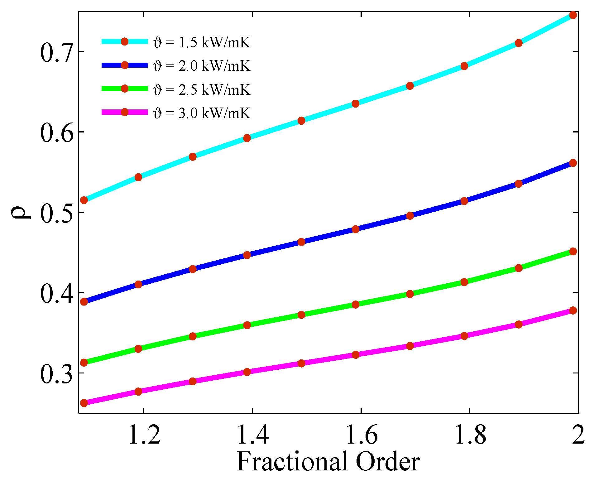
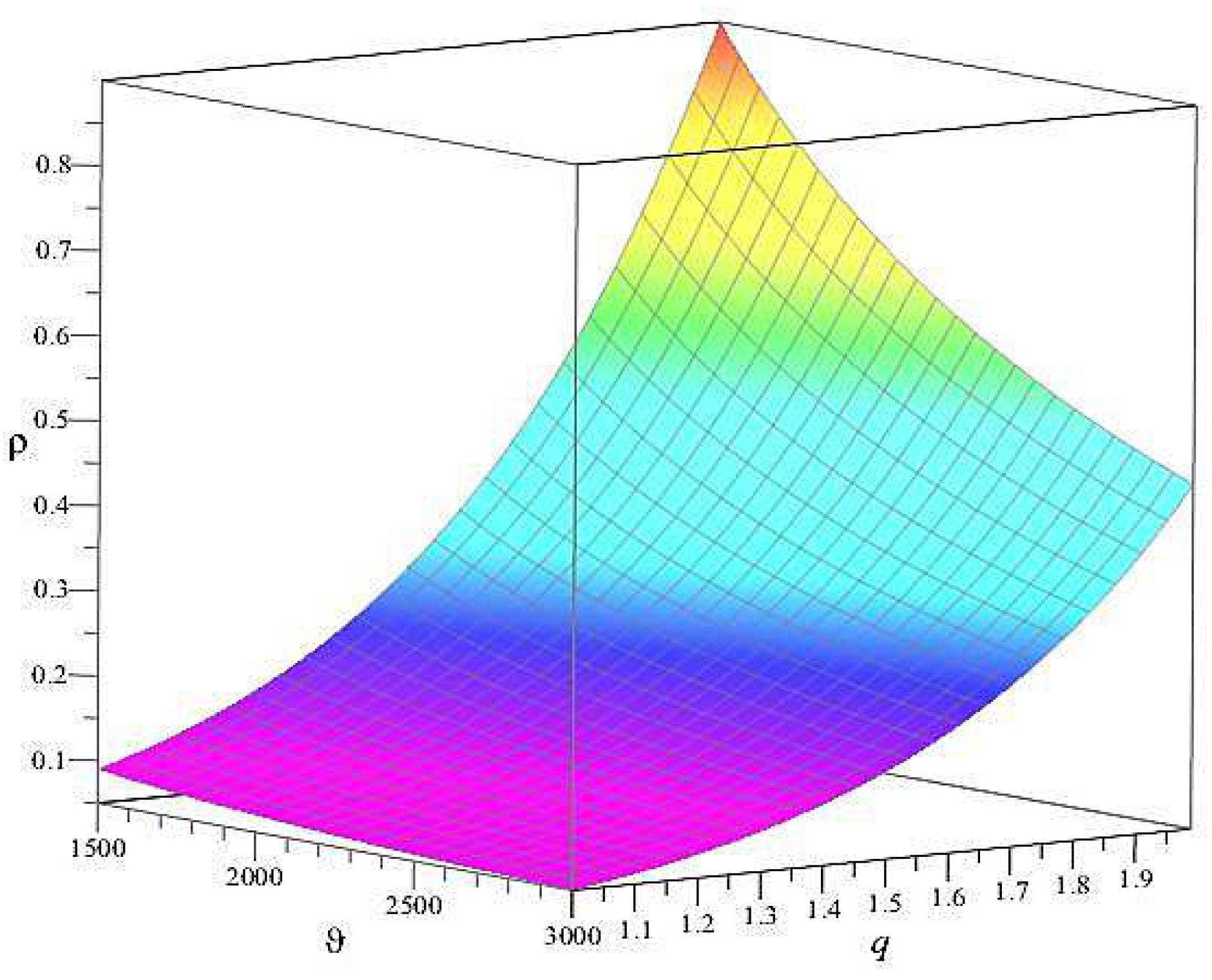
| 1.09 | 0.5148 | 0.3886 | 0.3129 | 0.2624 |
| 1.19 | 0.5435 | 0.4107 | 0.3301 | 0.2768 |
| 1.29 | 0.5690 | 0.4293 | 0.3454 | 0.2895 |
| 1.39 | 0.5922 | 0.4466 | 0.3593 | 0.3011 |
| 1.49 | 0.6138 | 0.4629 | 0.3723 | 0.3119 |
| 1.59 | 0.6351 | 0.4788 | 0.3851 | 0.3225 |
| 1.69 | 0.6573 | 0.4955 | 0.3984 | 0.3336 |
| 1.79 | 0.6819 | 0.5139 | 0.4131 | 0.3460 |
| 1.89 | 0.7106 | 0.5355 | 0.4304 | 0.3603 |
| 1.99 | 0.7453 | 0.5615 | 0.4512 | 0.3777 |
| 1.09000 | 1.1900 | 1.29000 | 1.3900 | 1.4900 | 1.5900 | 1.6900 | 1.7900 | 1.8900 | 1.9900 | |
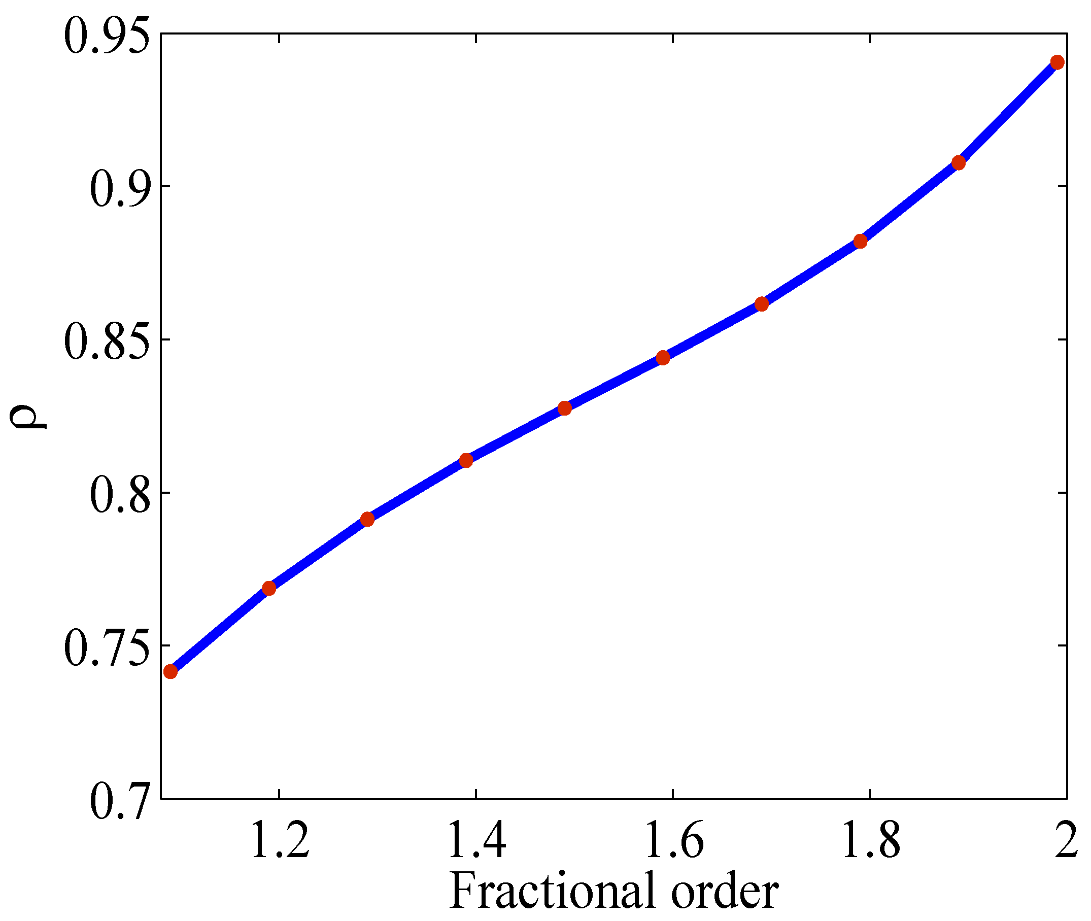
| 0.7416 | 0.7688 | 0.7913 | 0.8105 | 0.8275 | 0.8440 | 0.8616 | 0.8821 | 0.9077 | 0.9405 |
Publisher’s Note: MDPI stays neutral with regard to jurisdictional claims in published maps and institutional affiliations. |
© 2022 by the authors. Licensee MDPI, Basel, Switzerland. This article is an open access article distributed under the terms and conditions of the Creative Commons Attribution (CC BY) license (https://creativecommons.org/licenses/by/4.0/).
Share and Cite
Shammakh, W.; Selvam, A.G.M.; Dhakshinamoorthy, V.; Alzabut, J. Stability of Boundary Value Discrete Fractional Hybrid Equation of Second Type with Application to Heat Transfer with Fins. Symmetry 2022, 14, 1877. https://doi.org/10.3390/sym14091877
Shammakh W, Selvam AGM, Dhakshinamoorthy V, Alzabut J. Stability of Boundary Value Discrete Fractional Hybrid Equation of Second Type with Application to Heat Transfer with Fins. Symmetry. 2022; 14(9):1877. https://doi.org/10.3390/sym14091877
Chicago/Turabian StyleShammakh, Wafa, A. George Maria Selvam, Vignesh Dhakshinamoorthy, and Jehad Alzabut. 2022. "Stability of Boundary Value Discrete Fractional Hybrid Equation of Second Type with Application to Heat Transfer with Fins" Symmetry 14, no. 9: 1877. https://doi.org/10.3390/sym14091877
APA StyleShammakh, W., Selvam, A. G. M., Dhakshinamoorthy, V., & Alzabut, J. (2022). Stability of Boundary Value Discrete Fractional Hybrid Equation of Second Type with Application to Heat Transfer with Fins. Symmetry, 14(9), 1877. https://doi.org/10.3390/sym14091877