Symmetrization in the Calculation Pipeline of Gauss Function-Based Modeling of Hydrophobicity in Protein Structures

Abstract

In this paper, we show, discuss, and compare the effects of symmetrization in two calculation subroutines of the Fuzzy Oil Drop model, a coarse-grained model of density of hydrophobicity in proteins. In the FOD model, an input structure is enclosed in an axis-aligned ellipsoid called a drop. Two profiles of hydrophobicity are then calculated for its residues: theoretical (based on the 3D Gauss function) and observed (based on pairwise hydrophobic interactions). Condition of the hydrophobic core is revealed by comparing those profiles through relative entropy, while analysis of their local differences allows, in particular, determination of the starting location for the search for protein–protein and protein–ligand interaction areas. Here, we improve the baseline workflow of the FOD model by introducing symmetry to the hydrophobicity profile comparison and ellipsoid bounding procedures. In the first modification (FOD–JS), Kullback–Leibler divergence is enhanced with its Jensen–Shannon variant. In the second modification (FOD-PCA), the molecule is optimally aligned with the axes of the coordinate system via principal component analysis, and the size of its drop is determined by the standard deviation of all its effective atoms, making it less susceptible to structural outliers. Tests on several molecules with various shapes and functions confirm that the proposed modifications improve the accuracy, robustness, speed, and usability of Gauss function-based modeling of the density of hydrophobicity in protein structures.

1. Introduction

In the 1950s, Walter Kauzmann pioneered a perspective of a globular protein as a conglomerate of two zones [1,2], a hydrophobic interior (core) and a hydrophilic exterior (surface). In an analogy to a drop of oil poured into water—if no other factors intervene—the folding polypeptide should respond to the external stimulus of the aqueous environment in its own, sequence-encoded way by collapsing into a tightly packed conformation where hydrophobic residues bury under an insulating layer of their exposed polar counterparts [3,4]. This is the so-called hydrophobic effect [5]. Its involvement in the formation of complexes can be explained in a similar manner. Exposed hydrophobic residues stimulate the substrates to shield them from solvent, expelling H₂O molecules from the interface (although the final contact area can be mostly hydrophilic [6]). The hydrophobicity of amino acids is presented via scales like the well-known Kyte-Doolittle mapping [7].

Molecular simulations are indispensable computer techniques for the investigation of the structure, function, and other properties of biomolecular systems. They are commonly utilized in protein modeling and refinement, with molecular dynamics (MD) being their prime example [8]. There are two schemes of installation of aqueous environments in the simulation: explicit and implicit [9]. Explicit solvation places the protein in a box filled with many H₂O molecules_. They are precise but computationally expensive. Conversely, implicit models configure water as a continuous high-dielectric medium, enveloping the protein suspended in a void (low-dielectric) cavity carved to its size [10,11]. They greatly reduce the number of degrees of freedom in the system and nullify the need to track solvent–solvent interactions, resulting in a much faster calculation that permits longer MD time scales or larger structural inputs.

The performance of implicit solvation has motivated the development of many models [12]. In popular approaches, hydration-free energy is split between electrostatic and non-polar components, often expressing the second term via a function of solvent-accessible surface area (SASA) [12]. However, the status of the hydrophobic core is a function of the whole protein structure [13]. We need to consider the impact of the hydrophobic effect on all residues (i.e., everywhere from the molecule’s core to its surface), including their internal hydrophobic interactions. Due to the diversity of protein shapes and biological activities, a binary core vs. surface and polar vs. non-polar categorization cannot model this process with sufficient precision. Moreover, a molecule perfectly adhering to the ideal “oil drop” scheme would be completely soluble, with activity reduced to an inert presence. To carry out its function, it must exhibit some form of imperfection. If we could measure this irregularity, we could follow it to interesting parts of the structure, like active sites or protein–protein interface areas. This is where Fuzzy Oil Drop enters the scene.

Published in 2006 [14,15], Fuzzy Oil Drop (FOD) is an in silico model of distribution of hydrophobicity in protein structures. It can be seen as an “extension” of Kauzmann’s seminal idea. While it could also be classified as a coarse-grained, implicit solvation model, it is essentially a statistical method. In contrast to approaches measuring protein–water interactions at the SASA level, the FOD model relies on the general size of the void cavity containing that protein which it approximates with an ellipsoid—the titular drop. This drop is a vehicle for the expression of relation between the molecule and the aqueous environment (e.g., for hydrophobic core research) and for controlling the impact of the aqueous environment on that molecule (e.g., for folding simulations).

A polar residue can may find itself in the core, somewhere between core and surface, or its spatial neighborhood may belong on the opposite side of hydrophobicity scale, imposing its status. The remedy for this disparity is symbolized by “fuzzy” in FOD’s name. It refers to the turning of a discrete model into a continuous one. The 3D Gauss function (3DG) is utilized to express a measure of density of hydrophobicity that diminishes from the maximum in the center of the drop to nearly zero on its surface and beyond it, like water extends to infinity outside the void cavity. This measure can be likewise treated as the probability of finding of a hydrophobic residue at a given location in space. It is called the theoretical (idealized) distribution. This distribution is confronted via relative entropy with the so-called observed (empirical) distribution based on hydrophobicity scale and hydrophobic interactions between pairs of effective atoms representing the residues. It corresponds to the “real” state of the protein—what it folded to. In this way, the FOD model reaches beyond static hydrophobicity scales, enriching them with information encoded in the structure. The use of effective atoms (one per residue) explains its coarse graininess. It also means that it is not directly comparable with other solvation models as its measurements do not translate to energy terms. However, like force fields, it can act as an optimization objective or scoring function. For instance, hydrophobic effect can be simulated via the FOD model by gradually reducing the size of the drop, guiding an unfolded chain toward conformations where hydrophobic residues are buried in the core, and hydrophilic residues are exposed to the solvent.

Over the last 15 years, the FOD model has been used in various proteomic research topics [16], e.g., determination of the folding nucleus (in partnership with the Most Interacting Residues algorithm [17,18]) [19], analysis of the relation between structure and function [20], investigation of proteins involved in amyloid diseases (Aβ, Alpha Synuclein, Tau) [21], ab initio protein folding [22], building of a framework for non-bonded contact prediction via hydrophobicity density maps [23], and modeling of interaction with membranes [24]. This naturally incomplete list demonstrates the versatility of the modeling of the protein–water relationship by means of simple ellipsoid-based representation.

While a couple of interpretation schemes for FOD’s output were recently introduced [23,24], we have found that some computational aspects of this model can be likewise modernized (they were left unchanged for a long time, even since its inception in 2006), resulting in faster, more robust, and precise calculations that require less overseeing by their user. These findings are the motivation behind writing this paper. It is a major meta-analysis of the FOD model. Instead of using it in the usual research of hydrophobic core, we have focused here on its calculation pipeline, introducing optimizations to two subroutines: the comparison of hydrophobicity profiles (Section 3.1) and bounding of the input structure in the drop ellipsoid (Section 3.2). The changes we propose involve symmetrization that advances this model toward stronger conformance with its theoretical assumptions and opens it for further expansions. The first modification (FOD–JS) removes the ambiguity caused by the asymmetry of the current equation of relative entropy and reduces issues with values of hydrophobicity profiles close to or equal to zero. The second modification (FOD–PCA) ensures that the input set of effective atoms is optimally aligned with the axes of the coordinate system (diagonal covariance matrix) and adds a feature that counteracts artificial drop expansion due to structural outliers.

The results produced by the proposed modifications were compared with the output of an unmodified reference workflow here called the “baseline FOD algorithm”. It should be understood in all its steps from the preparation of the input structure to the calculation of entropy (described in Section 2.1). Derivative properties, such as additional profiles or hydrophobicity density maps [23,24], were not subject to this investigation. Tests were performed on a database of 12 proteins that appeared in our previous papers (three of them illustrate the related Ellipsoid Profile algorithm [25]). Structures in this set include simple helices, globular and non-globular monomers, multi-domain chains, and compact and massive complexes. They also exhibit various biological activities and distributions of hydrophobicity. To increase the number of inputs, we investigated a total of 32 of their fragments (chain from a complex, domain from a chain, complex of domains, etc.); details are in Section 2.2. This is not an exhaustive list of all molecules we have worked on so far, but a representative group exemplifying common types of inputs and outputs of the FOD model consisting of enough to present the outcome of its alternative algorithm.

2. Materials and Methods

2.1. The Fuzzy Oil Drop Model

This is a description of the baseline FOD algorithm. “Baseline” refers to all its steps from the preparation of the input protein to entropy-based profile comparison.

At first, the input structure must undergo the usual cleaning. This pertains to the removal of H₂O molecules and alternative atom locations other than those most often occupied. At this stage, our programs parse MODRES records present in the PDB header.

The next step involves selecting a part of the molecule for calculation. It is typically a domain, chain, or complex, but the FOD model can accept any collection of residues as long as their effective atoms are, at most, 9 Å away from at least one other effective atom. We explain this requirement in Section 3.1. An effective atom is understood here as a pseudo-atom placed at the mean position of all non-hydrogen atoms from the given residue. It represents that residue in space throughout the algorithm. It also means that the FOD model can work even with incomplete or Cα-only structures.

Selected residues were subsequently matched by their sequence with hydrophobicity parameters obtained from the hydrophobicity scale. The FOD model employs, by default, its own scale (0.0 < KEDQRNPSTGAHYLVMWIFC ≤ 1.0). Any non-negative mapping can be used here, although it naturally leads to different output of the algorithm. Non-standard amino acids must be excluded from the input unless they have entries on the scale or MODRES records resolve them to their standard parents. A common case is an approximation of selenomethionine (MSE) by methionine. This approach is favorable to the alternative which is a gap (i.e., missing data point) in the results.

The FOD model is tightly coupled with the concept of hydrophobicity density function that binds residues presented in sequence order with calculated values of hydrophobicity, forming a hydrophobicity profile. There are four such profiles in the baseline part of the algorithm, each carrying a different type of information. They are normalized to the 0–1 range and their length is equal to the number of selected residues, making them specific to the input structure. Their comparison allows for the quantitative measurement of how well this structure meets the model’s expectations. Accordance with the theory of FOD model corresponds to the detection of a stable, well-ordered hydrophobic core. Conversely, profile discrepancies can be examined in light of biological activity or non-bonded interactions at the quaternary structure level.

The first profile to calculate is H, the intrinsic hydrophobicity. It is simply a series of hydrophobicity parameters selected from the hydrophobicity scale, normalized by dividing them by their sum (H_sum). Hence, H ≡ {H₁…H_n}, where H_i is the value of the intrinsic hydrophobicity of the i-th residue, and n is the number of input residues. H denotes the status of the protein based solely on its sequence (e.g., in an unfolded polypeptide).

The next profile to calculate is O, the observed hydrophobicity. It expresses how intrinsic hydrophobicity of the residues is influenced by their neighboring residues in space. The intensity of this interaction is modeled after Michael Levitt’s sigmoid function [26]:

$$\mathrm{levitt}\left(i,j,c\right)=\left(H_i+H_j\right)\left[1-\frac{1}{2}\left(7{\left(\frac{r_{ij}}{c}\right)}^2-9{\left(\frac{r_{ij}}{c}\right)}^4+5{\left(\frac{r_{ij}}{c}\right)}^6-{\left(\frac{r_{ij}}{c}\right)}^8\right)\right]$$

(1)

i and j in {1…n} are indexes of residues, r_ij is the Euclidean distance between their effective atoms, and c = 9 Å is the assumed maximum range of hydrophobic interactions. The value of this polynomial starts at H_i + H_j when r_ij = 0 and reaches 0 when r_ij = c. Hence, O ≡ {O₁…O_n} where O_i is the value of observed hydrophobicity of i-th residue. It is equal to the sum of Equation (1) for i and all j ≠ i for which r_ij ≤ c. Like with H, each O_i is normalized by dividing it by the sum of all the values of the profile (O_sum). O denotes the status of the protein as seen only by itself (i.e., based on its sequence and structure).

The third profile to calculate is T, the theoretical hydrophobicity. It uses the 3D Gauss function to measure the aversion of residues to water depending on their spatial location:

$$\mathrm{gauss}\left(i,\mu ,\sigma \right)=\exp \left(\frac{-{\left(x_i-{\mu }_x\right)}^2}{2{\sigma }_x^2}\right)\exp \left(\frac{-{\left(y_i-{\mu }_y\right)}^2}{2{\sigma }_y^2}\right)\exp \left(\frac{-{\left(z_i-{\mu }_z\right)}^2}{2{\sigma }_z^2}\right)$$

(2)

i in {1…n} is an index of the residue, [x_i, y_i, z_i] is the XYZ position of its effective atom, [μ_x, μ_y, μ_z] is the mean position of all effective atoms, and [σ_x, σ_y, σ_z] is equal to ⅓ of lengths of radii of the drop (three sigma rule). The 3D Gauss function peaks at μ (which should be [0, 0, 0]) and reaches values close to 0 at 3σ and beyond. Hence, T ≡ {T₁…T_n}, where T_i is the value of theoretical hydrophobicity of i-th residue, equal to Equation (2). Identically to H and O, T is subject to normalization via its sum coefficient (T_sum). This profile denotes the sequence-independent relation of the protein with its environment.

The drop mentioned above is an ellipsoid surrounding the (assumed) globular shape of the molecule, which, in FOD’s theory, was reached in response to the presence of a solvent, guiding hydrophobic residues toward the interior and hydrophilic residues toward the outside. It is reflected by the T distribution. It has its maximum in the center of the drop and gradually decreases with its distance from it. The drop is fitted to the input structure in such a way that when centered at the origin and rotated so that its radii become parallel to the axes of the coordinate system, the variance of the effective atoms in all dimensions should be maximized. Lengths of those radii are determined by the longest absolute distances of aligned effective atoms from the origin in each dimension, all increased by 9 Å. See Section 3.2 for more detailed description of this procedure.

Because T, O, and H profiles are normalized and have the same length n, the input protein is now analyzable from FOD’s perspective by measuring their differences, both globally (for many residues) and at the local scale (for individual residues). Global analysis is based on Kullback –Leibler divergence (D_KL) [27]. Let P ≡ {P₁…P_n} and Q ≡ {Q₁…Q_n} be two discrete distributions of probability. Known as relative entropy, D_KL is a statistical distance expressing how P is different from Q (it is defined for continuous distributions too, but they are irrelevant here). For a pair of i-th elements of those distributions (P_i and Q_i), their D_KL-based distance is given by the following formula:

$${\mathrm{D}}_{\mathrm{KL}}\left(P_i|Q_i\right)=P_i{\log }_2\left(\frac{P_i}{Q_i}\right)$$

(3)

Applying the above equation to all i in {1…n} yields a series of D_KL values, which, when added together, denote the overall divergence between P and Q, D_KL(P|Q), understood as the amount of information (measured in bits) needed to encode P with Q:

$${\mathrm{D}}_{\mathrm{KL}}\left(P|Q\right)={\displaystyle \sum }_{i=1}^n{\mathrm{D}}_{\mathrm{KL}}\left(P_i|Q_i\right)$$

(4)

All FOD’s distributions of hydrophobicity are naturally predisposed to be P and Q. Hence, D_KL(O|T) is the divergence between O and T, which is conventionally shortened to O|T. D_KL(P_i|Q_i) = 0 if and only if P_i = Q_i. It is negative when P_i < Q_i, but D_KL(P|Q) is never below 0. It should be noted, however, that D_KL is a statistical distance, not a metric. This is because D_KL(P_i|Q_i) ≠ D_KL(Q_i|P_i) when P_i ≠ Q_i and D_KL(P|Q) = D_KL(Q|P) if and only if P ≡ Q (i.e., no symmetry). These properties are further discussed in Section 3.1.

The single, absolute value of entropy is meaningless as there is no universal threshold to decide when two hydrophobicity profiles are similar or different enough. Therefore, a reference measure of entropy is needed, obtained by replacing T in Equation (4) with R (a.k.a. random). R is the fourth and last hydrophobicity profile used by the baseline FOD. It describes a situation opposite to that modeled by the 3D Gauss function, when residues are indistinguishable from each other, expressing an identical (uniform) status. R is normalized by its definition, which means that R ≡ {R₁…R_n} and R_i = 1/n for all i in {1…n}.

The D_KL-based distance from O to R is likewise written as O|R. Its comparison with O|T confirms which of these two profiles the O profile is closer to at a global scale. It is simply that with lower divergence. However, to avoid the need to present and compare two numbers specific to the given input of the algorithm, the so-called Relative Distance coefficient (RD) was devised to bind them under a single value:

$$RD=\frac{O|T}{O\left|T+O\right|R}$$

(5)

RD assumes values between 0 (O ≡ T, full accordance with the theoretical model) and 1 (O ≡ R, full discordance), with 0.5 being the threshold between the observation of a stable hydrophobic core (RD < 0.5) and the absence of such stability (RD ≥ 0.5). The magnitude of this condition is expressed by the closeness of the protein to either end of the RD scale. This scale facilitates the comparison between structures when they are placed on it.

The T vs. R RD coefficient is the default, the most important RD status in the baseline FOD model. “Default” means that “RD” should be understood as Equation (5) (i.e., O|T vs. O|R) unless a specific context is given. This is because there is another RD variant. In this equation, R is sometimes replaced with H, resulting in O|H. D_KL then informs whether the O profile follows the sequence more closely than the 3D Gauss theory. To tell these two RDs apart, they are labeled as T-O-R and T-O-H, respectively.

The main concepts of the FOD model are visually presented in Figure 1 using catalytic domain of human Matrix Metalloproteinase-8 (PDB code: 1MMB [28]) as an example. This protein is a monomer with 158 residues and a mixed secondary structure. Its cartoon-style render is available in Figure S1. While it was not included in the main database of this work, and thus did not participate in the experiment, it nonetheless exhibits slight accordance with the model (T-O-R = 0.489). T-O-H = 0.508 suggests, on the other hand, that its O leans slightly more toward H than T, possibly due to the discrepancy between T and O in the central helix at L181-S202. This helix is involved in protein–ligand interaction and exhibits a status expected by FOD model for this type of interface (T ≫ O).

2.2. The Protein Database

The database of this work is composed of 12 proteins with various structures, functions, and distributions of hydrophobicity. All files were downloaded as usual from the Protein Data Bank (PDB) [29,30]. Their basic information is given in Table 1.

The PDB structures were broken into 32 fragments (domains, chains, complexes, etc.) which became the final input for the FOD algorithm in the experiment.

Table 2. Calculation input: fragments of proteins from Table 1 and their status. Underline denotes accordance (RD < 0.5).

PDB Code	Selected Fragment	RD T-O-R	PDB Code	Selected Fragment	RD T-O-R	PDB Code	Selected Fragment	RD T-O-R	PDB Code	Selected Fragment	RD T-O-R
1AON	A-U	0.799	1DIV	A(56-)	0.448	1J5B	A	0.767	2N0A	(A-J)(30-100)	0.531
1AON	A-N	0.793	1DIV	(A+B)(56-)	0.516	1LZ1	A	0.529	2N0A	A	0.733
1AON	O-U	0.746	1FXR	A+B	0.551	1TIT	A	0.425	2N0A	A(30-100)	0.568
1AON	A	0.771	1FXR	A	0.328	1XQ8	A	0.644	4B0H	A-C	0.585
1AON	U	0.625	1IIE	A-C	0.428	1XQ8	A(-100)	0.528	4B0H	(A-C)(-118)	0.500
1DIV	A+B	0.832	1IIE	(A-C)(-180)	0.494	1Y7Q	A+B	0.459	4B0H	A	0.472
1DIV	A	0.785	1IIE	A	0.553	1Y7Q	A	0.583	4B0H	A(-118)	0.382
1DIV	A(-55)	0.392	1IIE	A(-180)	0.623	2N0A	A-J	0.472	9MSI	A	0.292

presents residue ranges of those fragments and the RD status of their hydrophobic core (T-O-R in the sense of the baseline FOD model). All domain ranges were obtained from SCOP 2.08 database [31,32]. Additional details of the selected molecules and their high-resolution 3D renders can be found in Supplement File S1 (it also includes 1MMB from Figure 1).

Table 1. Proteins from the database. Exclamation mark (!) in chain length column denotes structures with number of residues available in PDB file lower than expected from their sequence. Data in Quaternary structure column refer to complex formation in author-assigned biological assembly. Asterisk (*) in this column marks structure recreated using symmetry operators from the PDB header, while values after hash (#) correspond to number of deposited solution NMR conformers (only model 1 was used in this experiment).

PDB Code	Molecule	Source Organism	Chain Length	Quaternary Structure	Ref.
1AON	GroEL/GroES chaperonin complex	Escherichia coli	547 aa! 97 aa	Homo-14-mer Homo-7-mer	[33]
1DIV	Ribosomal Protein L9	Bacillus stearothermophilus	149 aa	Homo-2-mer *	[34]
1FXR	Ferredoxin I (4F4S ligand)	Desulfovibrio africanus	64 aa	Homo-2-mer	[35]
1IIE	HLA-DR Invariant Chain	Homo sapiens	75 aa	Homo-3-mer (#20)	[36]
1J5B	Type I Antifreeze protein	Pseudopleuronectes americanus	38 aa!	Monomer (#20)	[37]
1LZ1	Lysozyme	Homo sapiens	130 aa	Monomer	[38]
1TIT	Titin I-band module	Homo sapiens	98 aa!	Monomer	[39]
1XQ8	Alpha Synuclein (micelle-bound)	Homo sapiens	140 aa	Monomer	[40]
1Y7Q	HIV Capsid C-Terminal Domain homologue	Homo sapiens	98 aa	Homo-2-mer (#20)	[41]
2N0A	Alpha Synuclein (pathogenic fibril)	Homo sapiens	140 aa	Homo-10-mer	[42]
4B0H	dUTPase YncF	Bacillus subtilis	144 aa!	Homo-3-mer	[43]
9MSI	Type III Antifreeze protein	Macrozoarces americanus	66 aa	Monomer	[44]

Table 1. Proteins from the database. Exclamation mark (!) in chain length column denotes structures with number of residues available in PDB file lower than expected from their sequence. Data in Quaternary structure column refer to complex formation in author-assigned biological assembly. Asterisk (*) in this column marks structure recreated using symmetry operators from the PDB header, while values after hash (#) correspond to number of deposited solution NMR conformers (only model 1 was used in this experiment).

PDB Code	Molecule	Source Organism	Chain Length	Quaternary Structure	Ref.
1AON	GroEL/GroES chaperonin complex	Escherichia coli	547 aa! 97 aa	Homo-14-mer Homo-7-mer	[33]
1DIV	Ribosomal Protein L9	Bacillus stearothermophilus	149 aa	Homo-2-mer *	[34]
1FXR	Ferredoxin I (4F4S ligand)	Desulfovibrio africanus	64 aa	Homo-2-mer	[35]
1IIE	HLA-DR Invariant Chain	Homo sapiens	75 aa	Homo-3-mer (#20)	[36]
1J5B	Type I Antifreeze protein	Pseudopleuronectes americanus	38 aa!	Monomer (#20)	[37]
1LZ1	Lysozyme	Homo sapiens	130 aa	Monomer	[38]
1TIT	Titin I-band module	Homo sapiens	98 aa!	Monomer	[39]
1XQ8	Alpha Synuclein (micelle-bound)	Homo sapiens	140 aa	Monomer	[40]
1Y7Q	HIV Capsid C-Terminal Domain homologue	Homo sapiens	98 aa	Homo-2-mer (#20)	[41]
2N0A	Alpha Synuclein (pathogenic fibril)	Homo sapiens	140 aa	Homo-10-mer	[42]
4B0H	dUTPase YncF	Bacillus subtilis	144 aa!	Homo-3-mer	[43]
9MSI	Type III Antifreeze protein	Macrozoarces americanus	66 aa	Monomer	[44]

Because we needed a simple convention for denoting the input, database proteins are referred to here mostly by their PDB codes using the following encoding scheme for their fragments: PDB_code:(chain_range)(residue_range), for example, 2N0A:(A-J)(30-100). It translates to “select residues with numbers 30 to 100 (inclusive) from chains A to J (inclusive) from structure 2N0A”. The beginning or end of the residue range can be omitted, e.g., 1XQ8:A(-100), which means that it starts or ends at the corresponding chain terminus. Whole chains are selected when that range is completely absent, e.g., 2N0A:(A-J). Without chains, the same residue range is selected from all chains, e.g., 2N0A:(30-100). If both parts are gone, we refer to the entire structure.

2.3. Principal Component Analysis

PCA is a statistical technique attributed independently in the early-twentieth century to Karl Pearson [45] and Harold Hotelling [46]. Given a set of n data samples, each described by d possibly related features (a d-dimensional vector), it finds a linear transformation to a new coordinate system where the mean of this data set is centered at the origin and the variance of the samples along all axes is maximized while the covariance matrix is diagonal [47]. This procedure permits information-preserving dimensionality reduction by keeping only a chosen number of the most varied projected features, known as principal components. PCA has a geometric analogue in fitting of an ellipsoid to d-dimensional point cloud by minimizing the orthogonal distance of those n points to its axes (i.e., the principal components) [47]. It can be efficiently calculated via singular value decomposition (SVD) which should be available in the popular numerical/statistical packages.

2.4. Tools and Websites

The 3D images of the proteins were rendered with PyMOL [48,49]. The charts were plotted using the Matplotlib library [50]. Our software modules employed state-of-the-art open-source Python libraries for scientific computation [51,52]. Online access to the Fuzzy Oil Drop model is available at http://fod.cm-uj.krakow.pl web server.

3. Results and Discussion

Two subsections comprise the Results section. They present and discuss the effects of modifications of the calculation pipeline of the baseline Fuzzy Oil Drop model proposed in this paper. The first modification (FOD–JS) introduces symmetrization to the hydrophobicity profile comparison subroutine, while the second (FOD–PCA) optimizes the procedure of the bounding of the input structure in the drop ellipsoid and adds a way to reduce the influence of structural outliers. The results are supported by explanatory and summary figures. Additional tables with numeric data are available in Supplement File S2.

3.1. Symmetrization in Hydrophobicity Profile Comparison (FOD-JS)

T, O, H, and R profiles express different categories of the density of hydrophobicity in the input structure. Each is normalized and has a length of n. Baseline FOD algorithm employs Kullback–Leibler divergence (D_KL) to quantitatively gauge differences between those profiles. To quickly reiterate Section 2.1, O|T symbolizes the D_KL-based distance from O to T. O|R is the coefficient for O and R (“random”). Relative Distance (RD) ties them together by placing the structure on a normalized 0–1 scale. When 0 ≤ RD < 0.5, O of this structure is closer to T (accordance with the model, well-ordered hydrophobic core), while 0.5 ≤ RD ≤ 1.0 is the evidence of O’s closeness to R (discordance, core’s instability). It is the default, most important, and the most used variant of RD in the baseline FOD algorithm, branded as T-O-R. Replacing R with H in Equation (5) yields T-O-H RD which reveals the position of O with respect to theoretical and intrinsic profiles. It is likewise possible to construct a third (but unused) variant of baseline RD, H-O-R.

D_KL is not a symmetric measure. This has a few consequences for its application in the comparison of profiles of hydrophobicity. First, it mandates a specific profile order for Equation (4). In the baseline FOD model, it is O|T, O|R, and O|H, which we shall call here the “O first” mode. The three reversed D_KL coefficients—namely T|O, R|O, and H|O (“O last”)— present the same profile relation but from the opposite perspective. They are unused in the baseline FOD model because equivalence cannot be expected between them (e.g., O|T ≠ T|O) in real proteins. The purpose of entropy in this context is to measure the difference between two profiles of hydrophobicity. The FOD model gives no special priority to residues with either T ≪ O or T ≫ O during this assessment. Put differently, an excess of hydrophobicity (T ≪ O) is not favored over its deficiency (T ≫ O) as the source of stronger discrepancy and vice versa. However, Equation (3) always favors one of them by assigning higher local divergence to residues exhibiting Q ≪ O in the “O first” mode and Q ≫ O in “O last” mode (Q = T/H/R). The mathematical basis behind this is presented in the next paragraph. However, this begs the question: which approach is more appropriate? First, second, or both? Hydrophobicity profiles often have shallower valleys below the R line compared to taller peaks above it, due to cysteine located at the top of the FOD model’s hydrophobicity scale, for instance. Their uneven treatment by relative entropy is beneficial as it prevents domination of the upper region. The drawback is that it applies to one profile at a time. The need for adherence to one mode (“O first”) also makes the RD calculation that does not involve the O profile cumbersome. For instance, if we wanted to measure the statistical distance between T and R, should we rely on T|R or R|T? This may likewise impede the introduction of new profiles.

The other problem with D_KL is numerical and relates to the handling of two side cases: the value of 0 and values close to 0. When P_i = Q_i = 0, Equation (3) becomes undefined, but because D_KL(P_i|Q_i) = D_KL(Q_i|P_i) = 0 if and only if P_i = Q_i, we can make an exception to return 0 directly, which is a correct and desirable approach. However, when P_i = 0 and Q_i > 0, Equation (3) also becomes undefined due to a lack of value of log₂0. We could try to avoid it by noticing that ${\lim }_{\mathrm{x}\to 0}$ x·log₂x = 0, thus assuming, by convention [53], that 0·log₂0 = 0. It circumvents the problem with the logarithm but introduces another in the form of 0 being reported when P_i ≠ Q_i. Likewise, P_i > 0 and Q_i = 0 results in division by zero or an assumption of infinity [53]. The fact that if P_i → 0 and Q_i > 0 then D_KL(P_i|Q_i) →0 and if P_i > 0 and Q_i → 0 then D_KL(P_i|Q_i) →∞ explains why the “O first” mode of comparison deems residues with O higher than the other profile as a source of higher local divergence and vice versa. We verify further down how different it actually is from “O last”.

Avoidance of 0 in the observed profile is the reason why every effective atom must be located within a 9 Å of at least one other effective atom in the input. While this requirement should be satisfied by all valid and (mostly) complete protein structures, it is nonetheless an unnecessary obstacle, making it harder to experiment with residue selections or values of c. To prevent 0 from appearing in H (and possibly in O), we had to increase at one point the hydrophobicity parameter of lysine to 0.001 and use enough significant digits in the textual output of the algorithm to avoid issues with rounding.

D_KL’s lack of an upper bound means that a small profile change close to 0, undetectable by humans and irrelevant from the perspective of the overall stability of the hydrophobic core, can boost local divergence, assigning undue importance to affected residues. It may be detrimental to the optimization of protein structures (i.e., folding simulation or prediction of complex formation), which is carried out with FOD by finding the state of the system that corresponds to the lowest statistical distance between T and O.

From the perspective of a programmer, an inadvertent profile switch during a call to a function that calculates D_KL (e.g., T swapped with O) produces perfectly valid code and results that are disastrous for conclusions regarding the status of the hydrophobic core. Because such mistake may go unnoticed until much later, extra care is needed during access to this part of the FOD library. Finally, plots of the D_KL series are inherently unintuitive with their mix of positive and negative values.

All above problems can be solved or strongly diminished by “promoting” D_KL to D_JS, the so-called Jensen–Shannon divergence [54]. D_JS is a symmetric variant of Kullback–Leibler entropy, averaging the statistical distance from P_i and Q_i to their average (a):

$${\mathrm{D}}_{\mathrm{JS}}\left(P_i|Q_i\right)=\frac{1}{2}\left[{\mathrm{D}}_{\mathrm{KL}}\left(P_i|a\right)+{\mathrm{D}}_{\mathrm{KL}}\left(Q_i|a\right)\right], a=\frac{1}{2}\left(P_i+Q_i\right)$$

(6)

$${\mathrm{D}}_{\mathrm{JS}}\left(P|Q\right)={\displaystyle \sum }_{i=1}^n{\mathrm{D}}_{\mathrm{JS}}\left(P_i|Q_i\right)$$

(7)

Like D_KL, D_JS(P_i|Q_i) = 0 if and only if P_i = Q_i and D_JS(P|Q) = 0 if and only if P ≡ Q. It also has a few other useful properties [55,56,57,58]. The first is its aforementioned symmetry: D_JS(P_i|Q_i) = D_JS(Q_i|P_i) and D_JS(P|Q) = D_JS(Q|P). The second is its non-negativity and its upper bound: 0 ≤ D_JS(P_i|Q_i) ≤ 1 and 0 ≤ D_JS(P|Q) ≤ 1. The third is that its square root is a proper metric—it satisfies triangle inequality. Finally, owing to being a sum of two factors, it can gracefully handle appearance of 0 anywhere in the compared distributions. To verify that, once again we need to assume that 0·log₂0 = 0 [53]. We can then rewrite Equation (6) by incorporating Equation (3) directly in it:

$${\mathrm{D}}_{\mathrm{JS}}\left(P_i|Q_i\right)=\frac{1}{2}\left[P_i{\log }_2\left(\frac{2P_i}{P_i+Q_i}\right)+Q_i{\log }_2\left(\frac{2Q_i}{P_i+Q_i}\right)\right]$$

(8)

Now, without loss of generality, if we assume that P_i = 0 and Q_i > 0, we obtain:

$${\mathrm{D}}_{\mathrm{JS}}\left(0|Q_i\right)=\frac{1}{2}\left[0+Q_i{\log }_2\left(\frac{2Q_i}{0+Q_i}\right)\right]=\frac{1}{2}{Q}_i{\log }_{2}2=\frac{Q_i}{2}$$

(9)

Setting P_i = 0 thus yields a divergence equal to half of Q_i—the mean of Q_i and 0. If we replace the second half of that sum with 0 when Q_i = 0, 0 will be returned automatically for D_JS(0|0), thus requiring only two special cases to properly manage all three variants with 0. It also means that, unlike the unbound D_KL, Equation (6) cannot reach values higher than half the maximum of P and Q, making it predictable and placing its human-readable plot in the same (or scaled down) value range as its input distributions.

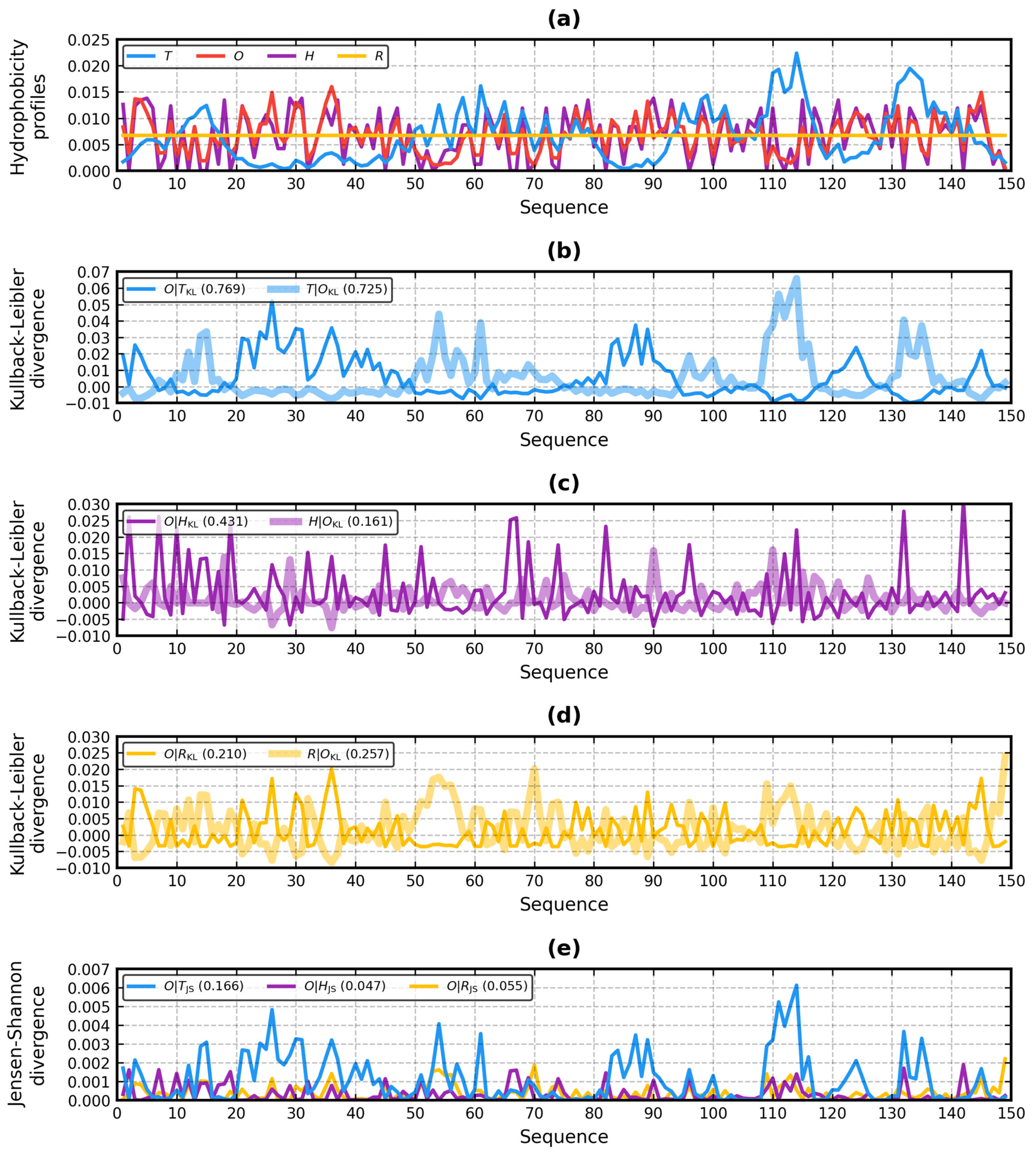
Figure 2 presents the results of the application of the above theory in practice. It displays a comparison between T, O, H, and R profiles in 1DIV:A via D_KL and D_JS.

Because hydrophobicity profiles of the FOD model are now comparable using two measures of entropy, we had to introduce new symbols in this paper to tell them apart: O|T_KL, O|T_JS, T-O-R_KL, T-O-R_JS, and others. Their meaning should be obvious.

Due to two domains and non-globular conformation, 1DIV:A is highly discordant with the model, as confirmed by T-O-R_KL = 0.785 and T-O-H_KL = 0.641. Furthermore, when one looks closely at Figure 2b–d, it becomes clear that the “O first” D_KL series—D_KL(O|T), D_KL(O|R), and D_KL(O|H)—indeed reports higher local divergence for residues where O is above the other profile. It is very noticeable in the G107-L117 region where a prominent T peak contributes a tiny, negative bend to O|T, while in the N20-T40 region, T is below O yet it achieves top values of D_KL(O|T) (Figure 2b). Both views are reversed in the “O last” D_KL series—D_KL(T|O), D_KL(R|O), and D_KL(H|O). It resulted in these values: O|T_KL = 0.769, T|O_KL = 0.725, O|R_KL = 0.21, R|O_KL = 0.257, O|H_KL = 0.431, and H|O_KL = 0.161.

T and O, which disagree the most in 1DIV:A (Figure 2a), exhibit smallest arithmetic difference between their alternative D_KL perspectives with O|R and R|O closely behind them in this sense. However, O|H is nearly three times higher than H|O. An explanation can be found again in Equation (3). When O_i is higher than H_i and T_i which are also closer to 0, the values of D_KL(O_i|T_i) and D_KL(O_i|H_i) must increase. K132 and K142 make good examples of this phenomenon, showing relatively tall peaks in Figure 2c. Reversing profile order in Equation (4) has a small to medium effect on O vs. T and O vs. R and a strong effect on O vs. H due to the fact that O and T are less often closer to 0 than H. Moreover, the O profile of 1DIV:A looks reasonably similar to the H profile. It is not far from reality, since by definition, O highly depends on its source. The contribution of the nearest (H_i±1) neighbors in the sequence to O_i can reach up to 50% in a typical protein. However, is O really closer to R than to H in this structure as O|H and Figure 2d are implying? D_JS can help alleviate this ambiguity by joining pairs of opposing D_KL views in a similar manner to how RD binds the compared coefficients together. Coincidentally, they even have the same value range. In this sense, Jensen–Shannon “equalizes” Kullback–Leibler by raising peaks everywhere the compared profiles differ (e.g., for both N20-T40 and G107-L117 regions in Figure 2e), thus marking the residues exhibiting discrepancy while maintaining a balance of importance between the excess and deficiency of hydrophobicity. It resulted in the following pairs of values of Equation (7): O|T_JS = 0.166 = T|O_JS, O|R_JS = 0.055 = R|O_JS, and O|H_JS = 0.047 = H|O_JS. Calling upon Equation (5) reveals the final hydrophobic core status in 1DIV:A in the sense of both measures of entropy: T-O-R_KL = 0.785, T-O-R_JS = 0.749, T-O-H_KL = 0.641, T-O-H_JS = 0.778, H-O-R_KL = 0.672, and H-O-R_JS = 0.460.

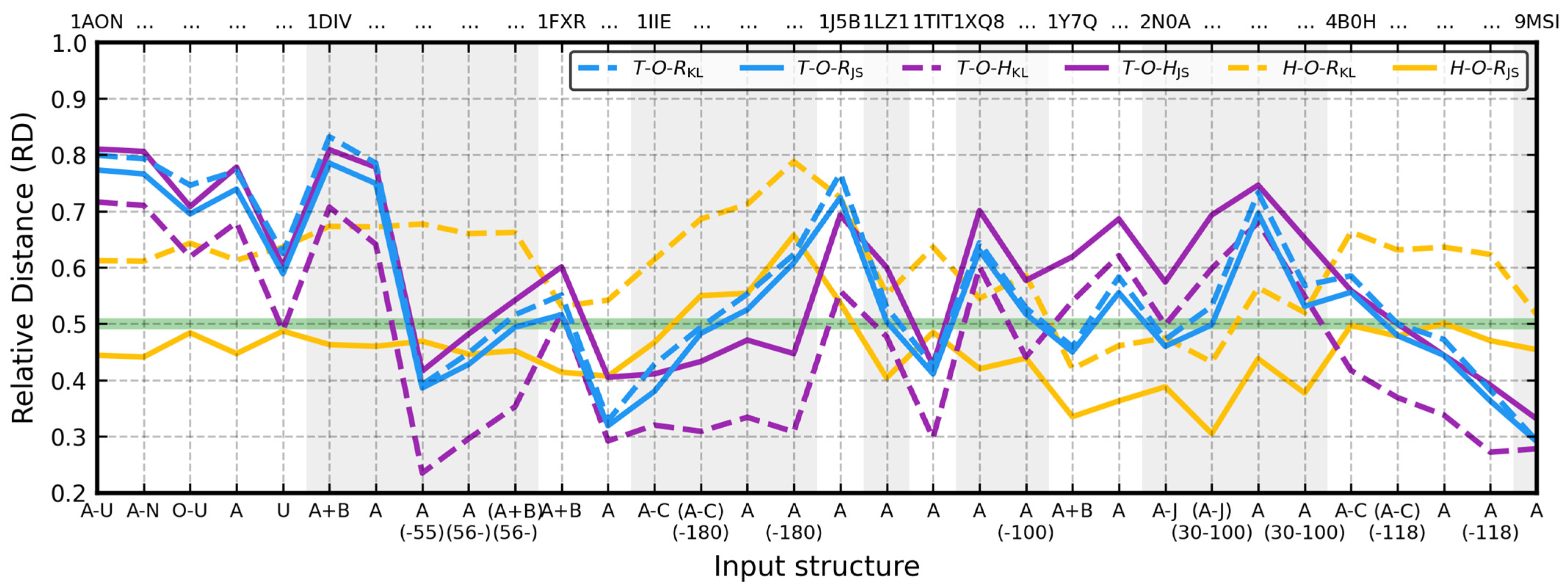
Experimental data for all proteins from the database can be found in Table S1 and are plotted in Figure 3. Each of the 32 inputs from Table 2 was individually subject to the FOD model’s calculation and the status of its hydrophobic core was measured with D_KL and D_JS. Results in the form of Figure 2 are available in Supplement File S3.

Among the 32 test inputs, 11 had T-O-R_KL < 0.5, 18 had T-O-H_KL < 0.5, and only 4 had H-O-R_KL < 0.5. Switching to D_JS caused a mean change of T-O-R in the database by 0.025 (T-O-R_KL−T-O-R_JS, σ = 0.013). Accordance with the model remained the same in 29 cases. The three that became accordant (T-O-R_JS < 0.5) were 1DIV:(A+B)(56-), 2N0A:(A-J)(30-100), and 4B0H:(A-C)(-118). In this group, 1DIV:(A+B)(56-) and 4B0H:(A-C)(-118) were initially closest to 0.5 (4B0H:(A-C)(-118) even had T-O-R_KL = T-O-H_KL = 0.500), so it is not surprising. However, the accordance of the central part of 2N0A (T-O-R_JS = 0.498) is not a favorable outcome. We correct it in Section 3.2. O|T_KL and T|O_KL were similar in each input, with an average ratio of 1.011 (σ = 0.105). Lower T-O-R_JS was caused by O|R_KL being, on average, 0.83 of R|O_KL (σ = 0.05). The same conclusion can be arrived at by noticing that the mean O|T_KL / O|T_JS and T|O_KL / O|T_JS ratios are 4.28 (σ = 0.305) and 4.252 (σ = 0.249), but the mean O|R_KL / O|R_JS and R|O_KL / O|R_JS ratios are 3.799 (σ = 0.078) and 4.587 (σ = 0.197). When O|T decreases and O|R increases, Equation (5) mandates that T-O-R must decrease toward accordance with the T profile, here by a maximum of 0.051 in 1AON:(O-U) and a minimum of 0.001 in 9MSI. The correlation coefficient between T-O-R_JS and T-O-R delta was measured in the entire test suite at 0.58.

O|H_KL was nearly the double of H|O_KL in the database (μ = 1.935, σ = 0.394), owing to average values of O|H_KL / O|H_JS and H|O_KL / O|H_JS ratios equal to 7.135 (σ = 1.078) and 3.726 (σ = 0.210), respectively. Joining them in O|H_JS and putting them against O|T_JS resulted in an increase in T-O-H_JS in every case (μ = 0.113, σ = 0.033). It may seem to be a lot, but O switched to H’s side of the RD scale (T-O-H_JS ≥ 0.5) only seven times, in 1AON:U, 1DIV:(A+B)(56-), 1LZ1, 1XQ8:A(-100), 2N0A:(A-J), 4B0H:(A-C), and 4B0H:(A-C)(-118). 1XQ8:A(-100) evened the classification of its hydrophobic core with 1XQ8 and unveiled K21 and K80 which face the center of the drop as highly discordant. Omitting them causes its core to gain stability (T-O-R_KL = 0.497, T-O-R_JS = 0.481). The highest RD change (0.189) was observed this time in 1DIV:(A+B)(56-) with the lowest shift once again reported by 9MSI (0.053). It can be attributed to the high values of the H profile in this structure (away from 0—it has only a single lysine, K61), resulting in comparable O|H_KL and H|O_KL (0.118 vs. 0.126). The other two pairs of its D_KL coefficients also exhibit similarities. It makes sense for a type III antifreeze molecule.

The four inputs that were closer to H than to R in terms of D_KL (H-O-R_KL < 0.5) were 1Y7Q:(A+B), 1Y7Q:A, 2N0A:(A-J), and 2N0A:(A-J)(30-100). D_JS caused this observation to nearly reverse. H-O-R_JS was reduced in all database structures by 0.149 (σ = 0.038) on average, resulting in all but five test cases—1IIE:(A-C)(-180), 1IIE:A, 1IIE:A(-180), 1J5B, and 4B0H:A—flipping their accordance from R to H (H-O-R_JS < 0.5). The highest and lowest RD deltas were again found in 1DIV:(A+B)(56-) and 9MSI, respectively (0.21 and 0.062). It is a natural consequence of the findings from previous paragraphs; when O|R increases while O|H decreases, H-O-R must go down. This coefficient complements the “RD triangle” in which T, H, and R are vertexes and T-O-R, T-O-H, and H-O-R are edges of length 1 on which O can slide. An interesting relation between this trio can be seen in Figure 3; H-O-R is below 0.5 when T-O-R is below T-O-H and vice versa with both D_KL and D_JS. In fact, H-O-R can be approximated as 0.5+(T-O-R)-(T-O-H). Correlation coefficients between these two values were measured in the database at 0.987 for D_KL and 0.996 for D_JS. In some cases, their absolute difference was less than 1 × 10⁻⁴ (1FXR, 1LZ1, 2N0A, 4B0H), while elsewhere it reached up to 0.017~0.048 with D_KL (1AON, 1DIV, 1IIE) and up to 0.014~0.019 with D_JS (1AON, 1DIV).

While unused by the baseline FOD model, H-O-R can nonetheless measure by how much T-O-R and T-O-H differ and how strongly the intrinsic hydrophobicity of residues (H) is affected by their local spatial neighborhood in the structure (expressed by O) without consideration for the surrounding water (i.e., it is unaffected by the drop size).

3.2. Symmetrization in Bounding in Drop Ellipsoid (FOD-PCA)

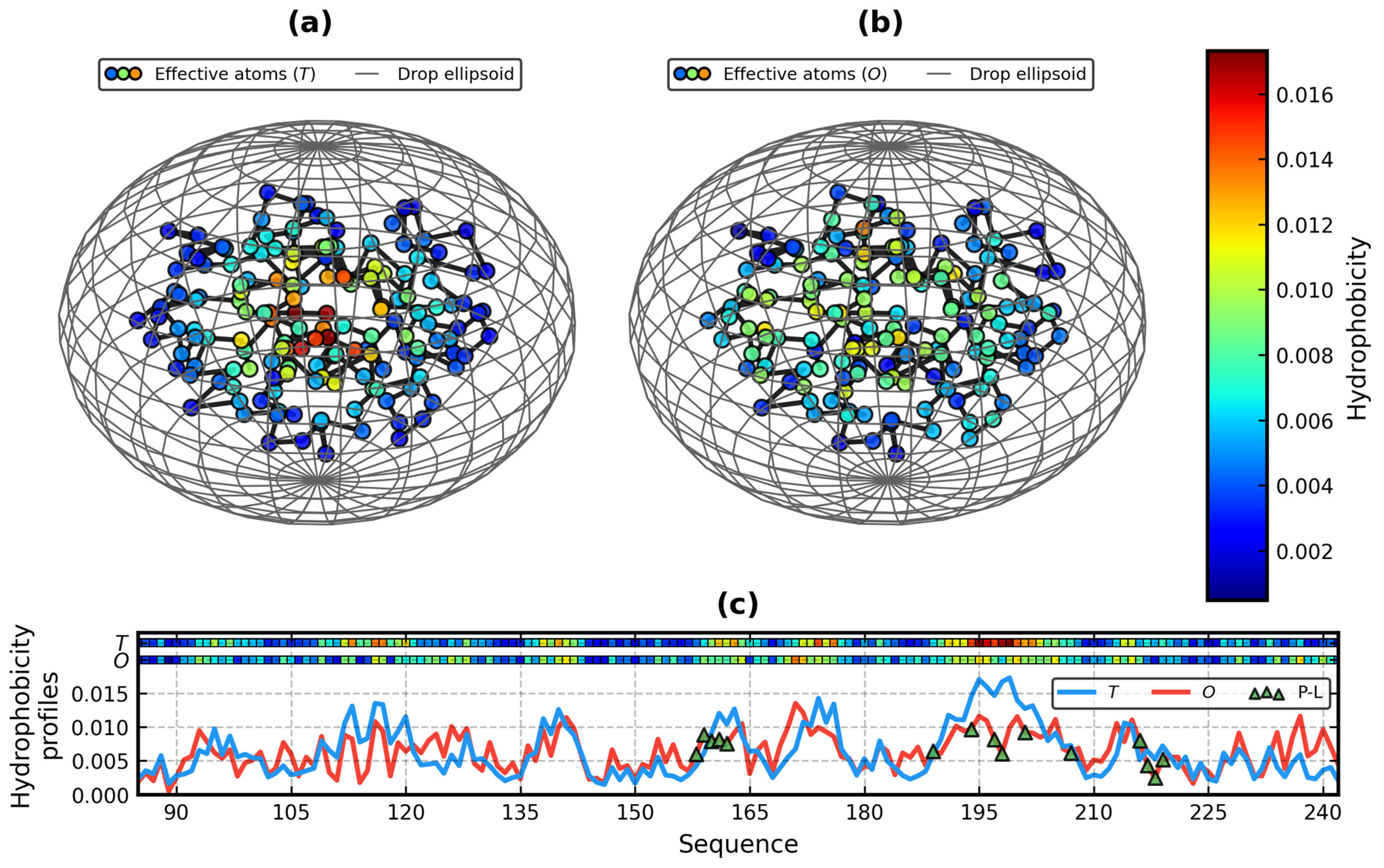
To calculate its T profile, the input protein must be bound inside an axis-aligned ellipsoid (drop) which represents this protein’s relationship with the surrounding aqueous environment. The first part of this procedure involves the translation of effective atoms to the origin and their rotation in alignment with the axes of the coordinate system in a way that maximizes their variance in all dimensions. The second step determines the size of the drop—the lengths of its radii constituting the basis for standard deviation parameters passed to Equation (2). O distribution, which is based solely on the hydrophobicity scale and pairwise hydrophobic interactions between residues, is naturally invariant to the spatial orientation of the input as a whole.

The baseline FOD algorithm for axis alignment and drop radii selection has the following description: after the translation of the mean position of all effective atoms to the origin, their most distant pair in 3D is found, and the whole set is rotated so that line connecting that pair becomes parallel to the X-axis. Next, effective atoms are orthogonally projected onto the YZ plane and rotated again, this time around the X-axis. The line connecting their most distant pair found in this plane must then become parallel to the Y-axis. The alignment step is complete. Both searches can be significantly accelerated by noticing that their solutions must belong to the convex hulls of the input data.

Absolute positions of effective atoms located furthest away from the origin in each dimension, all three extended by 9 Å, mark the final lengths of the radii of the drop. The three sigma rule allows the 3D Gauss function to reach nearly 0 at its surface and beyond, while the 9 Å radii extension counteracts domination over the whole profile by residues located near the origin, stretching it, and lowering its values. Drop size has a strong impact on theoretical hydrophobicity. The effects of its alterations (e.g., growing or shrinking) are more noticeable in small molecules than in large complexes.

The baseline approach works reasonably well in typical cases, particularly when the largest spread of effective atoms is sufficiently approximated by the line going through their most distant pair. However, sometimes it produces highly suboptimal alignments. It happens when structural outliers (e.g., disordered chain termini) disturb that balance. They are normally withdrawn a priori from the input structure by hand, for instance, by trimming 4B0H:A to 4B0H:A(-118). It is done because complete immersion in the solvent prevents those fragments from contributing much to the stability of the hydrophobic core in the main (globular) part of the molecule. Unfortunately, their manual removal is not feasible during bulk calculation when hundreds of structures pass through the algorithm. Any procedure of their detection must also consider the fact that in non-globular proteins, all or nearly all residues exhibit the same, low effective atom density (e.g., in 1XQ8).

The presence of outlier fragments has yet another, even more, severe consequence. They cause the drop to artificially inflate, misrepresenting the status of the hydrophobic core of the protein due to the overly stretched T profile. 1IIE, 1Y7Q, 2N0A, and 4B0H are examples of such structures in the database. On the other hand, a lack of outliers does not guarantee a lack of suboptimal alignment. It can still occur when most distant pairs of effective atoms coincide with the diameter of the structure more than with their largest spread. Again, it happens because the baseline alignment process relies only on that pair while everything else is ignored. The GroEL molecule from 1AON is a perfect example of this issue. Results of its baseline ellipsoid bounding are shown in Figure 4a–c. To correct the ≈45° rotation in the XY plane, a manual selection of the longest axis of the drop is required, for instance, by averaging two sets of effective atoms located at opposite sides of the molecule (e.g., residues with the same number from different chains, honoring axial symmetry). It works but requires the user’s active participation. Likewise, Figure 4d–f illustrates how disordered outliers in 2N0A (outside the central A30-L100 region) skew its alignment with both a wrong angle and an overly spacious drop. It is more appropriate to leave some residues out of the drop—like the aforementioned highly exposed outliers—than grow it too large to keep them all inside (unless, of course, one wishes to encompass the structure exactly like it is). All distributions of the FOD model allow that.

Sometimes it happens that two or more chains with an identical sequence and nearly identical tertiary structure report conflicting coefficients from opposite halves of the RD scale. Even if they stay on the same side, the different status of individual residues may perturb their classification via hydrophobicity density maps. 1Y7Q exemplifies such RD disparity in the database. Monomers in its NMR conformer 1 that was used in this experiment exhibit T-O-R_JS of 0.555 (chain A) and 0.534 (chain B) owing to the short bent N-terminal region in the second structure (G35-D41). Their RMSD is only 0.6 Å.

Ellipsoid bounding of 1AON:(A-N) and 2N0A:(A-J) presented in Figure 4g–l is not encumbered by the difficulties mentioned above. Their structures are aligned in accordance with the model’s and user’s expectations. Axial symmetry of GroEL is properly discovered, while outlying segments of amyloid fibril do not interfere with finding the largest spread of effective atoms in the A30-L100 region. They are partially pushed out of the drop, providing a tighter, more accurate fit to the central part of the molecule (as it turns out, also in terms of RD). These results were obtained via an alternative alignment method based on principal component analysis and a modified drop size selection scheme. They are the focus of this part of the paper (see Section 2.3 for a general description of PCA).

Unlike the baseline alignment algorithm which relies on the longest distance between effective atoms, the PCA-based approach considers them all, delivering optimal translation vector and rotation matrix which position the input data set at origin and rotate it in a way that truly (rather than approximately) maximizes variance in each dimension. Put differently, a diagonal 3 × 3 covariance matrix is produced. 1AON:(A-N) illustrates this very well. On Figure 4a–c, σ²(x) = 1548.7, σ²(y) = 1401.6, σ²(z) = 1234.3, cov(x,y) = 247.3, cov(x,z) = −75.7, and cov(y,z) = −52.4, while on Figure 4g–i, σ²(x) = 1749.5, σ²(y) = 1220.8, σ²(z) = 1214.2, and the rest of matrix is zero. As a beneficial side effect, taking all effective atoms into account allows PCA to automatically (i.e., without the user’s intervention) discover symmetry in the molecule, even in the highly disordered 2N0A:(A-J) (Figure 4j–l). This is exactly what the theoretical hydrophobicity of the FOD model expects to be done with its effective atoms. Aligning them with PCA is also faster than the baseline approach between 6 and 9 times (≈7 on average, σ ≈ 0.4). The speed-up magnitude naturally depends on the computer environment, but it omits an additional and more complicated algorithm (convex hull) and a subsequent search among pairs of elements of its output.

At this moment, effective atoms are aligned with axes of the coordinate system. Now it is time to choose the right size of the drop. The baseline algorithm relies for that on the longest distance to the origin in each dimension, which in turn relies on only up to three effective atoms, making it subject to potential drop radii length overestimation, especially along the Y- and Z-axes. Since it can be problematic for working with small structures, we would like to alleviate this problem or at least diminish its severity.

PCA only provides radii direction vectors (principal components) of the ellipsoid fit to the input data, but not their lengths. It is left to the user to decide at which size this ellipsoid separates the interior model from exterior outliers. In the FOD model, it must encompass the molecule in a manner that approximates its assumed globular shape, not too large and without carving too much into the structure. If the spread of effective atoms is utilizable to achieve their optimal axis alignment, it can be used to determine drop size as well. Drop radii are sought on behalf of theoretical distribution which models the distribution of residues via a multivariate normal distribution. Hence, their lengths can be determined from standard deviations of effective atoms in each dimension (σ_x, σ_y, σ_z) and the value from the χ² distribution with three degrees of freedom at confidence level P [59]. The point [x, y, z] belongs then to the surface of an axis-aligned ellipsoid when:

$${\left(\frac{x-{\mu }_x}{{\sigma }_x}\right)}^2+{\left(\frac{y-{\mu }_y}{{\sigma }_y}\right)}^2+{\left(\frac{z-{\mu }_z}{{\sigma }_z}\right)}^2=s={\chi }_{\left(P,3\right)}^2$$

(10)

Because [μ_x, μ_y μ_z] = [0, 0, 0], to obtain the radius of this ellipsoid in the X dimension, y and z need to be set to 0, resulting in x = σ_x√s and so on for y and z.

We realized, however, that the above approach may, in turn, overestimate x after the standard deviation along the X-axis is maximized, while too small value of P can produce too small drops. Hence, we decided to combine its anti-outlier properties with the baseline method. After the PCA-based alignment, the modified drop radii were set in this experiment to an average of baseline radii and the results of Equation (10) with P = 0.75 (s ≈ 4.108, √s ≈ 2.027, very close to 2σ) and then extended by 9 Å. Whether this protocol can be further optimized is something to discover in another paper. Drops shown as red ellipses in Figure 4g–l were obtained by adhering to it. They are nearly identical to baseline radii (the orange ellipses) for 1AON:(A-N), but visibly shorter for 2N0A:(A-J).

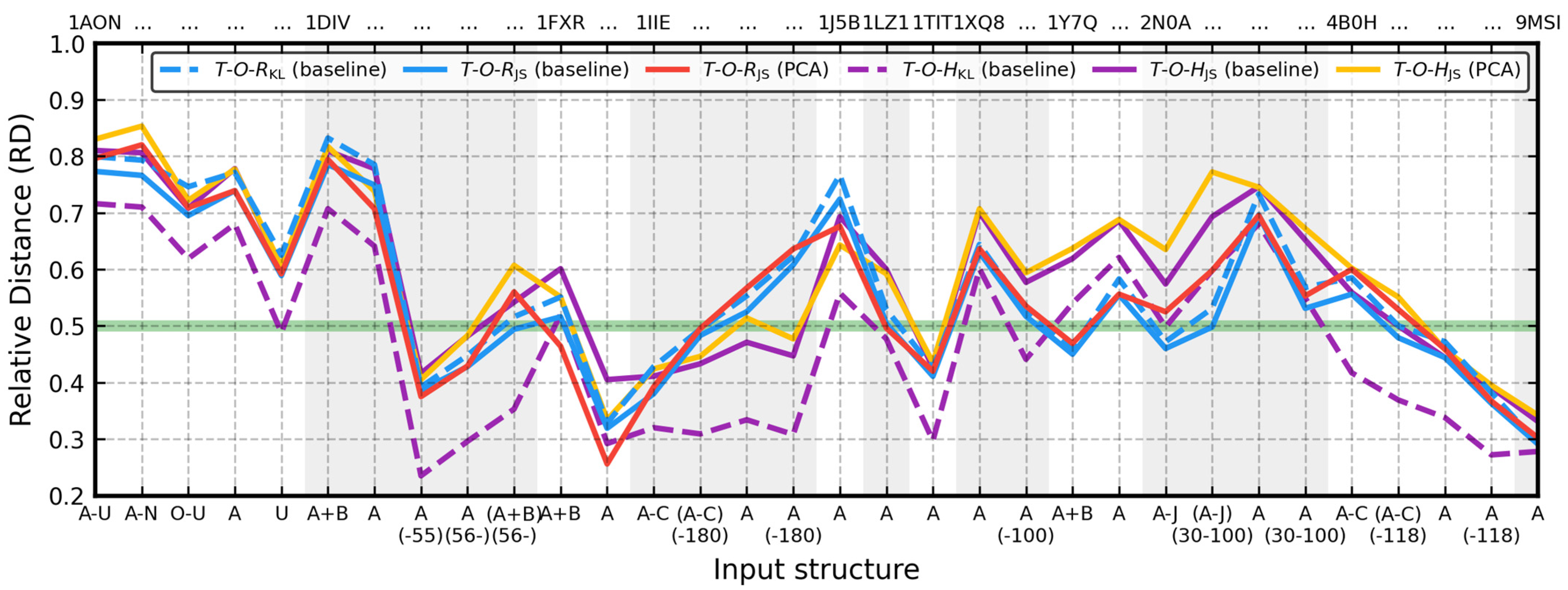
Experimental data for all proteins from the database can be found in Tables S2 and S3 and are plotted in Figure 5. Each of the 32 inputs from Table 2 was individually subject to the FOD model’s calculation following a separate baseline and modified bounding in the drop ellipsoid after which the status of its hydrophobic core was measured with D_KL and D_JS. Additionally, we checked the post-alignment standard deviations of the effective atoms and the sizes of the drops (radii length and volume coefficient V = r_x·r_y·r_z/1000). The comparison of those drops in a form similar to Figure 4 is available in Supplement File S4.

As expected, PCA-based alignment produced a diagonal effective atoms covariance matrix for all test cases. In comparison to the baseline approach, it maximized their standard deviation along the X-axis and decreased it along the Y- and Z-axes, reaching, on average, 102.7% (σ = 3.2%), 99% (σ = 5.1%), and 92.7% (σ = 7.1%) respectively. It resulted in slightly smaller drops, confirmed by these average modified/baseline ratios: r_x/r_x = 94.9% (σ = 5.7%), r_y/r_y = 91% (σ = 8.6%), r_z/r_z = 91.1% (σ = 6.9%), and V/V = 79.1% (σ = 12%). When 1IIE:(A-C), 1Y7Q:(A+B), 2N0A:(A-J), and 4B0H:A (i.e., inputs with significant outliers) are discounted, these ratios change to 95.7% (σ = 5.4%), 92.4% (σ = 8%), 92% (σ = 6.7%), and 81.4% (σ = 10.5%). The only protein in which the V coefficient was increased, although just by 3%, was 1J5B. The r_x/r_x ratio exceeded 1 five times and was exceeded the most in 1DIV:A (1.07) and 1J5B (1.08). Conversely, drops of even longer 1X8Q and 1XQ8:(-100) remained akin to their baseline counterparts. The same happened to globular inputs: 1AON:(O-U), 1AON:U, the domains of 1DIV:A, 1IIE:A(-180), 1TIT, 4B0H:A(-118), and 9MSI. Automated alignment correction to properly handle the structural symmetry and a drop shrink resulting from it was observed in 1AON:(A-U), 1AON:(A-N), 1AON:A, 1DIV(A+B), 1DIV:A, 1DIV:(A+B)(56-), 1FXR:(A+B), 1IIE:(A-C), 1IIE:(A-C)(-180), 1Y7Q:(A+B), 2N0A:(A-J), and 2N0A:(A-J)(30-100).

Unstructured outlier chain segments were managed by the modified FOD algorithm in all four test cases in which they were prominently exposed to the solvent: 1IIE:(A-C), 1Y7Q:(A+B), 2N0A:(A-J), and 4B0H:A. By managed, we mean counteracting their negative influence by reducing size of the drop toward a correct approximation of the dense part of the structure—the assumed location of the hydrophobic core. We do not consider the S181-K192 region of 1IIE:A as an outlier because of the short length of this chain (75 aa) and its loose tertiary structure. In this sense, it is closer to 1XQ8 and 2N0A:A which lack any tertiary structure. Thus, terminal regions in those inputs (and in 1XQ8:A(-100)) should not be classified as different from the rest in terms of effective atom density. Our modification recognizes that and does not needlessly shrink their drops. On the other hand, its use resulted in the following V/V ratios (modified / baseline): 058 for 1IIE:(A-C), 0.73 for 1Y7Q:(A+B), 0.53 for 2N0A:(A-J), and 0.66 for 4B0H:A. However, 1AON:(A-N) obtained 0.63, and 2N0A:(A-J)(30-100) obtained 0.47 because of the correction of their alignment. This gave us, however, an idea as to how we can detect and report the possible presence of outliers in the input. Effective atoms should be first aligned with the PCA-powered approach and then the V/V ratio calculated for drops with radii lengths chosen using modified and baseline methods (e.g., red vs. orange on Figure 4g–l). This changes the above numbers to 0.73 for 1IIE:(A-C), 0.75 for 1Y7Q:(A+B), 0.6 for 2N0A:(A-J), 0.79 for 4B0H:A, 1.01 for 1AON:(A-N), 0.82 for 2N0A:(A-J)(30-100), and 0.84 for 1IIE:A.

The average RD difference between baseline (D_KL) and modified (D_JS) bounding was measured at 0.013 (σ = 0.038) for T-O-R, −0.125 (σ = 0.048) for T-O-H, and −0.149 (σ = 0.038) for H-O-R. H-O-R is the same as in Section 3.1 as only the T profile was altered here. Omitting 1IIE:(A-C), 1Y7Q:(A+B), 2N0A:(A-J), and 4B0H:A causes these values to change to 0.015 (σ = 0.038) for T-O-R, −0.126 (σ = 0.05) for T-O-H, and −0.155 (σ = 0.036) for H-O-R. With D_KL replaced by D_JS, baseline and alternative approaches differ on average by −0.013 (σ = 0.035) in terms of T-O-R and −0.011 (σ = 0.033) in terms of T-O-H. Without structures with outliers, both RD variants report a mean change of ≈−0.01 (σ ≈ 0.035).

Jensen–Shannon entropy caused three inputs to accord with the model in Section 3.1 (T-O-R_JS < 0.5): 1DIV:(A+B)(56-), 2N0A:(A-J)(30-100), and 4B0H:(A-C)(-118). PCA-based alignment and alternative drop size selection took them back to the discordant side of the RD scale. This is particularly beneficial with the amyloid which received higher T-O-R_JS (0.598 vs. 0.531) than before. 2N0A:(A-J)—the complete fibril—also “fixed” the baseline status of its hydrophobic core: to T-O-R_JS = 0.525 from T-O-R_KL = 0.472. This time it was 1FXR:(A+B) and 1LZ1 which switched to accordance with the model, suggesting that the Ferredoxin I complex of two highly stable monomers is actually stable (T-O-R_JS = 0.464)—a change of core status classification caused by an alignment correction mostly in the XZ plane. 1DIV:(A+B)(56-) reports a similar rotation fix, only in the XY and XZ planes and with the opposite effect on perception of its stability. 1FXR:A also became the most stable structure in the database (T-O-R_JS = 0.256), overtaking 9MSI (T-O-R_JS = 0.302).

The situation with T-O-H did not change much. Only 1IIE:A joined the seven structures that moved closer to H in Section 3.1 (T-O-H_JS ≥ 0.5), confirming a stronger impact on this coefficient by the symmetric measure of entropy rather than by manipulation of the drop. More interesting is the fact that RD coefficients calculated for monomers of 1Y7Q were brought closer to each other. T-O-R_JS changed from 0.555 to 0.556 for chain A and from 0.534 to 0.554 for chain B, overcoming RD discrepancy caused by the 1Y7Q:B(35-41) region. T-O-H_JS for chain A changed from 0.686 to 0.688 and from 0.641 to 0.659 for chain B, reducing the RD difference by ≈35%. T-O-R_JS of 1Y7Q:(A+B) remained similar to value of this coefficient for its structure with outliers removed from it a priori (0.469 vs. 0.472). It is a very promising outcome. A similar phenomenon was observed for its T-O-H_JS, but to a lesser extent as expected (0.637 vs. 0.654). We also noticed that in the entire NMR ensemble of 1Y7Q (all 20 conformers), the standard deviation of T-O-R_JS was reduced by 9.5% for the dimer, by 4.8% for chain A, and by 16.7% for chain B. For T-O-H_JS, these ratios were measured at 16.7%, 12.5%, and 8.7%, respectively.

4. Conclusions

This paper reports our findings regarding the modification of two portions of the calculation pipeline of the Fuzzy Oil Drop model. We propose these changes to overcome some of the issues present in the baseline FOD algorithm, optimize, modernize, and prepare it for possible further enhancements. They were named FOD–JS and FOD–PCA to make it easier to reference them in the future and to hint at what they do. Through uncomplicated practical solutions, we were able to guide this model toward stronger conformance with its own theoretical premises. The main theme of this work and the key to achieving this goal is symmetrization.

Upgrading the Kullback–Leibler divergence to its symmetric Jensen–Shannon variant supplies the hydrophobicity profile comparison subroutine with several benefits (FOD–JS modification). By merging pairs of alternative and normally unequal D_KL views (e.g., O|T_KL and T|O_KL), D_JS points to all regions of the sequence where both types of profile discrepancy occur (e.g., T ≪ O and T ≫ O), providing a unified source of information in which to search for interesting residues, for example, the most important members of the hydrophobic core or those engaged in the protein–protein interaction. Moreover, D_JS removes ambiguity from this process (e.g., O|T_JS = T|O_JS) and avoids the need to conform to a particular profile order in Equation (4), greatly reducing the chance of a programmer’s mistake and permitting any profile pair to be compared by dropping the requirement for the participation of O in Equation (5).

O|T_KL was comparable with T|O_KL in many test proteins, suggesting that the switch from D_KL to D_JS is relatively innocuous for conclusions involving T-O-R. One can expect the baseline classification of the status of the hydrophobic core (side of RD scale) to be maintained by FOD–JS, but there are exceptions. The situation regarding T-O-H is different because of a stronger impact of H|O_KL on O|H_JS. It resulted in a universal increase of this variant of RD but not to the point of causing an accordance flip in more than a few inputs. Nevertheless, in our opinion, higher T-O-H is a more befitting representation of the high reliance of the O distribution on intrinsic hydrophobicity.

Unlike D_KL, D_JS gracefully handles the appearance of 0 anywhere in the hydrophobicity profiles, whether it appears there deliberately or due to unexpected factors. D_JS is also much less affected by values of hydrophobicity close to 0—its peaks raise at a controllable rate to a predictable upper limit within a value range of the input distributions. By knowing that theoretical maximum (i.e., half of the highest value in the compared profiles), we can use it to choose a threshold for finding local peaks of entropy. A visual inspection of plots in Supplement File S3 suggests that 10% of that maximum might be a feasible solution. For instance, 9MSI with its T and O reaching up to ≈0.03 has no D_JS peaks over 0.0015 (as it should, given its low T-O-R), while peaks corresponding to the largest profile discrepancies in 1AON:U (both T ≪ O and T ≫ O) surpass 0.00125 (10% of ≈0.025) over a span of several residues. This fairly simple detection scheme could be further expanded by introducing a sequence dimension to the equation (i.e., peak width).

PCA-based alignment absolves the user of the model from overseeing the bounding of the input molecule in the drop (FOD–PCA modification). Even in highly disordered structures like 2N0A, symmetry is discovered automatically, resulting in optimal orientation of effective atoms (diagonal covariance matrix) needed for their proper portrayal by the 3D Gauss function. 1AON no longer requires manual selection of the longest axis of its drop. This procedure is parameter-free, trivial to implement, and faster than the baseline approach by nearly an order of magnitude, allowing more CPU time to be dedicated to other tasks, for example, to the nearest neighbor search during O profile calculation.

By relying on the standard deviation of all effective atoms instead of their maximum distance to the origin, FOD–PCA reduces the sensitivity of the drop radii length selection subroutine to structural outliers, such as disordered chain termini freely moving in the solvent. 1Y7Q is a very good example. Its drop is no longer inflated too much to contain the protruding N-terminal region in chain B, resulting in nearly equalized RD for monomers and a status of the dimer close to when those outliers are a priori removed from it. This procedure has a single parameter—confidence level P controlling the size of the ellipsoid generated via Equation (10). We set P = 0.75 in this experiment (which corresponds to ≈2 multiplication factor for the standard deviation of effective atoms) and averaged the resulting radii with the baseline radii calculated after the PCA-based alignment. This approach seems to work well for all test cases. It yields neither too small nor too large drops, allowing it to be called a safe default. To verify its effects on particularly elongated structures, we generated a straight 50 aa alanine peptide and the longest drop radius difference between FOD–PCA and baseline methods was ≈9 Å. The other two radii were nearly identical and T-O-R_JS was in both cases above 0.9. On top of that, drop size comparison grants a way to estimate whether outliers exist in the input. The 0.75~0.8 volume coefficient ratio (V_modified/V_baseline) seems to be a feasible threshold for this purpose.

Like the other implicit solvation models [60], the FOD model has its limits too. In the Introduction, we mentioned that its measurements do not translate into terms of energy used by typical force fields. It highly depends on size of the drop and may eventually need to incorporate other biomolecular properties that can likewise contribute to the status of the hydrophobic core. With the advent of D_JS-based profile comparison, it should be easy to express those properties in the same form as the currently employed distributions.

Online access to the FOD algorithm with the choice between the baseline and the alternative calculation modes is available at http://fod.cm-uj.krakow.pl web server.