


Dark Energy from Virtual Gravitons (GCDM Model vs. ΛCDM Model)

Abstract
1. Introduction
2. Dark Energy from Virtual Gravitons
3. Distance Modules
4. GCDM vs. ΛCDM
5. What Are the Prospects for the GCDM Testing and Comparison with ΛCDM Model?
6. Transition Redshifts
7. Conclusions
Author Contributions
Funding
Institutional Review Board Statement
Informed Consent Statement
Data Availability Statement
Acknowledgments
Conflicts of Interest
Appendix A. Outline of Graviton Theory of Cosmological Acceleration
Appendix B. Bogoliubov–Born-Green–Kirkwood–Yvon Hierarchy (BBGKY Chain)
Appendix C. Integration of BBGKY Chain
Appendix D. Why Now? Why the Dark Energy of Graviton Origin Should Appear in the Matter-Dominated Era?
Appendix E. About Early Dark Energy
| 1 | Quoted from [67]. |
| 2 | In fact, the history of the cosmological constant from its inception in 1917 to the present day is an exciting “astronomical adventure novel,” detailed in a beautifully written historical and astronomical study [67]. |
| 3 | It worth to note that even big enough at the point leads to a picture similar to Figure 4. |
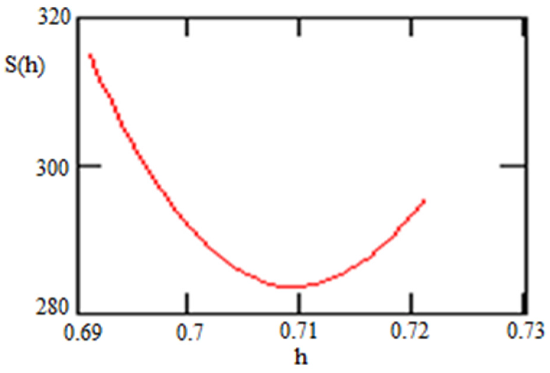
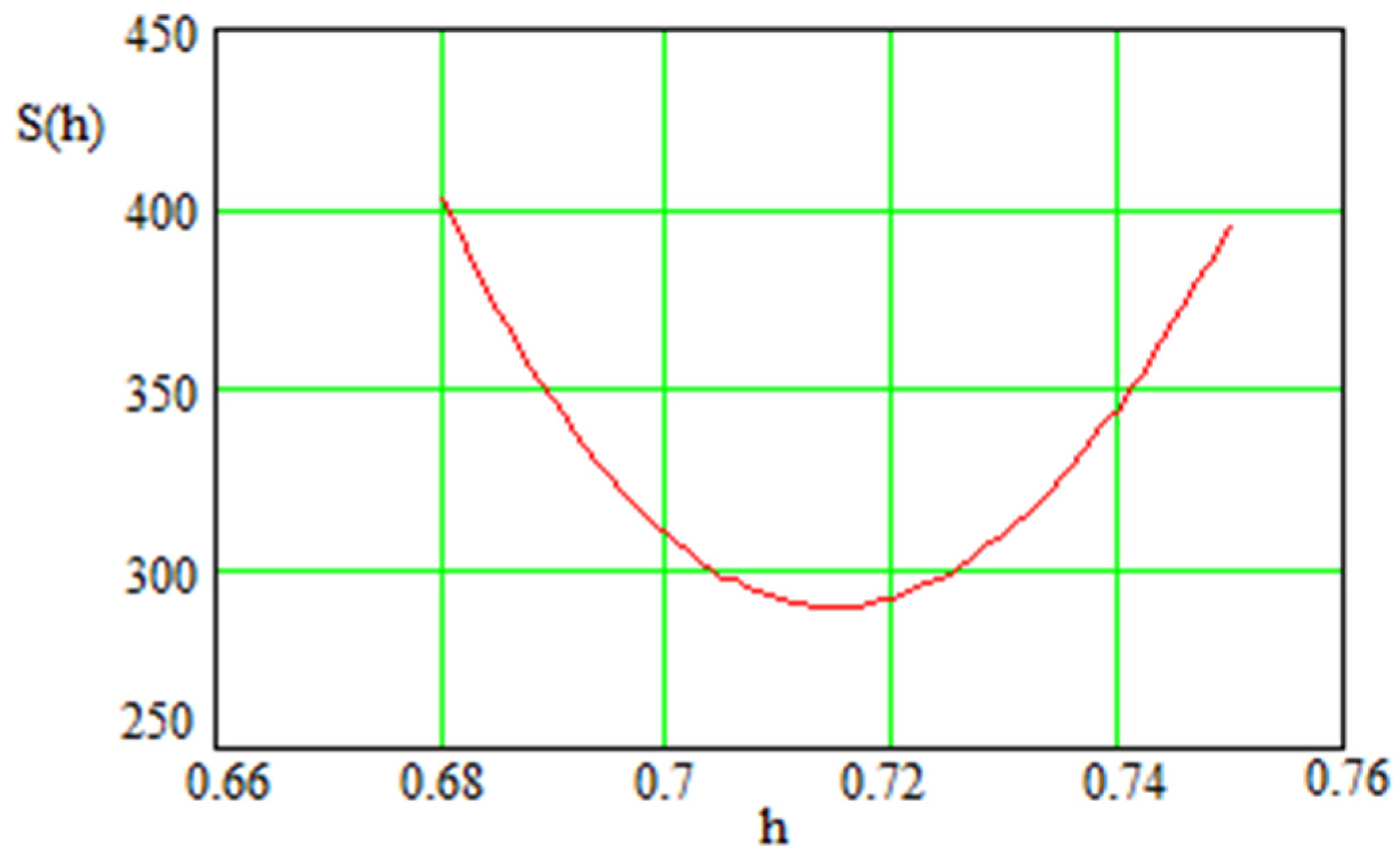
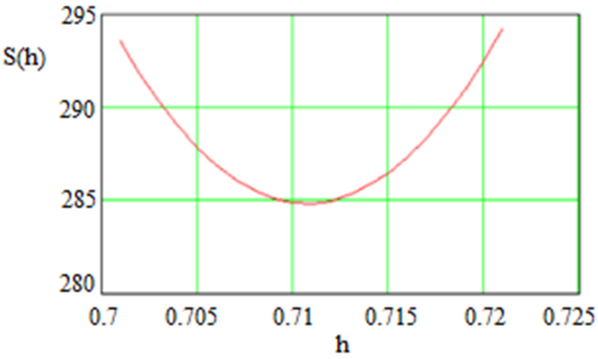
| 4 | The tension between numerical value of Hubble constant H was a subject for intense discussion between two research groups [68,69]. The last publication of Freedman [43] shows that the last measurement of h gives H0 = 69.8 ± 0.6 (stat) ± 1.6 (sys) km/s/Mpc. Note that we obtained h = 0.71 as a number minimizing the statistical sums for the cosmological constant for all three cases, which is closed to Freedman’s h = 0.698. |
| 5 | |
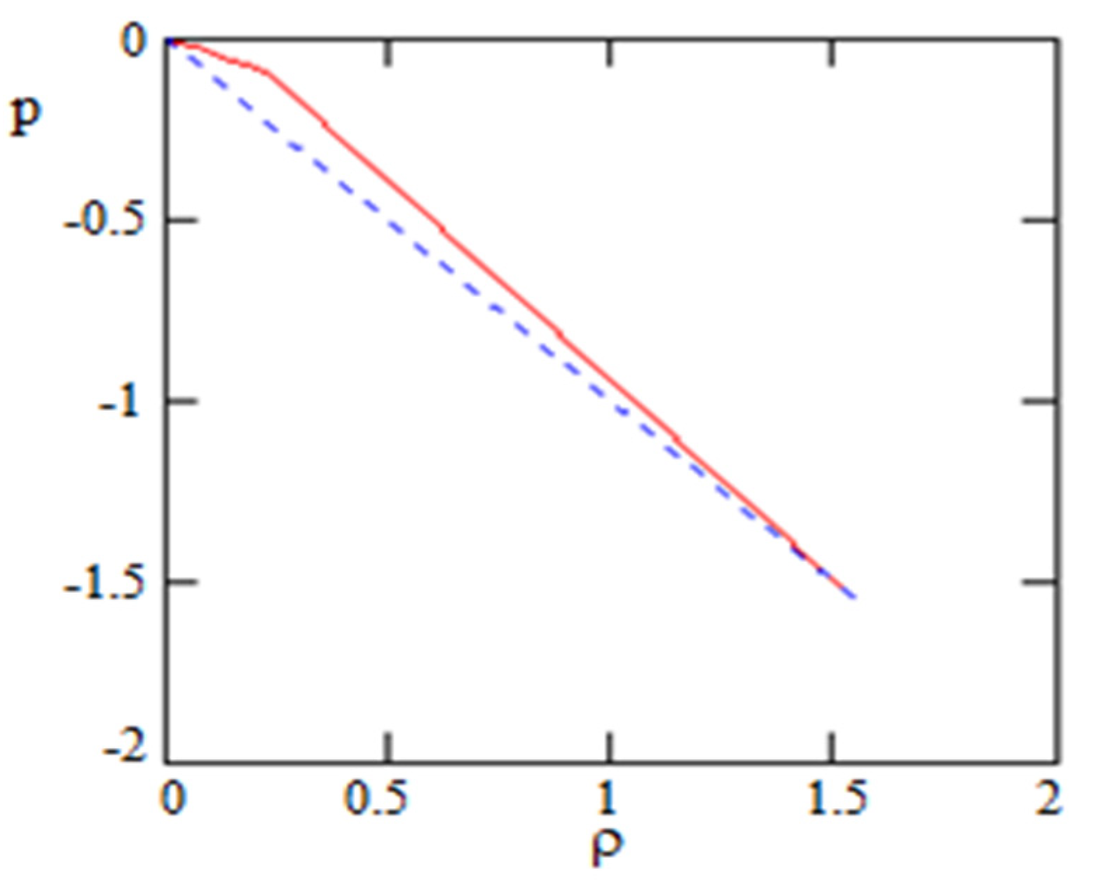
| 6 | In our current paper, we added the non-relativistic matter with the equation of state p = 0 (see below). |
| 7 |
References
- Riess, A.G.; Filippenko, A.V.; Challis, P.; Clocchiatti, A.; Diercks, A.; Garnavich, P.M.; Gilliland, R.L.; Hogan, C.J.; Jha, S.; Kirshner, R.P. Observational evidence from supernovae for an accelerating universe and a cosmological constant. Astron. J. 1998, 116, 1009–1038. [Google Scholar] [CrossRef]
- Perlmutter, S.; Aldering, G.; Goldhaber, G.; Knop, R.A.; Nugent, P.; Castro, P.G.; Deustua, S.; Fabbro, S.; Goobar, A.; Groom, D.E.; et al. Measurements of Ω and Λ from 42 high-redshift supernovae. Astrophys. J. 1999, 517, 565–586. [Google Scholar] [CrossRef]
- Kamenshchik, A.Y.; Moschella, U.; Pasquier, V. LambdaCDM epoch reconstruction from F (R, G) and modified Gauss-Bonnet gravities. Phys. Lett. B 2001, 511, 265–268. [Google Scholar] [CrossRef]
- Bento, M.; Bertolami, O.; Sen, A. Generalized Chaplygin gas, accelerated expansion, and dark-energy-matter unification. Phys. Rev. D 2002, 66, 043507. [Google Scholar]
- Carroll, S.M. The Cosmological Constant. Living Rev. Relativ. 2001, 4, 1. [Google Scholar] [CrossRef]
- Mukhanov, V. Physical Foundations of Cosmology; Cambridge University Press: Cambridge, UK, 2005. [Google Scholar]
- Copeland, S.E.G.; Sami, M.; Tsujikawa. Dynamics of dark energy. S. Int. J. Mod. Phys. D 2006, 15, 1753–1936. [Google Scholar] [CrossRef]
- Weinberg, S. Cosmology; Oxford University Press: Oxford, UK, 2008. [Google Scholar]
- Chernin, A.D. Dark energy and universal antigravitation. Phys. Uspekhi 2008, 51, 253–282. [Google Scholar] [CrossRef]
- Yoo, J.; Watanabe, Y. Theoretical models of dark energy. Int. J. Mod. Phys. D 2012, 21, 1230002. [Google Scholar] [CrossRef]
- Heisenberg, L. A systematic approach to generalisations of General Relativity and their cosmological implications. arXiv 2018, arXiv:1807.01725v1. [Google Scholar] [CrossRef]
- Wetterich, C. Cosmology and the fate of dilatation symmetry. Nucl. Phys. B 1988, 302, 668. [Google Scholar] [CrossRef]
- Caldwell, R.; Dave, R.; Steinhardt, P.J. Cosmological imprint of an energy component with general equation of state. Phys. Rev. Lett. 1998, 80, 1582–1585. [Google Scholar] [CrossRef]
- Caldwell, R.; Linder, E.V. Limits of quintessence. Phys. Rev. Lett. 2005, 95, 1401. [Google Scholar] [CrossRef]
- Verlinde, E. Emergent gravity and the dark universe. SciPost Phys. 2017, 2, 016. [Google Scholar] [CrossRef]
- Alexander, S.; Cortês, M.; Liddle, A.R.; Magueijo, J.; Sims, R.; Smolin, L. Cosmology of minimal varying Lambda theories. Phys. Rev. D 2019, 100, 083507. [Google Scholar] [CrossRef]
- Zel’dovich, Y.B. The cosmological constant and the theory of elementary particles. Sov. Phys. Usp. 1968, 11, 381–393. [Google Scholar] [CrossRef]
- Hoyle, F.; Burbidge, G. Relation between the Red-shifts of Quasi-stellar Objects and their Radio Magnitudes. Nature 1966, 212, 1334. [Google Scholar] [CrossRef]
- Longair, M.; Scheuer, P.A.G. Red-shift magnitude relation for quasi-stellar objects. Nature 1967, 215, 919–922. [Google Scholar] [CrossRef]
- Burbidge, G.; Burbidge, E. Absorption lines in quasi-stellar objects. Nature 1967, 216, 1092–1093. [Google Scholar] [CrossRef]
- Petrosian, V.; Salpeter, E.; Szekeres, P. Quasi-stellar objects in universes with non-zero cosmological constant. Astrophys. J. 1967, 147, 1222–1226. [Google Scholar] [CrossRef]
- Shklovsky, J. On the nature of" standard" absorption spectrum of the quasi-stellar objects. Astrophys. J. 1967, 150, L1–L3. [Google Scholar] [CrossRef]
- Kardashev, N. LemaItre’s Universe and Observations. Astrophys. J. 1967, 150, L135–L139. [Google Scholar] [CrossRef]
- Rowan-Robinson, M. On cosmological models with an antipole. Mon. Not. R. Astron. Soc. 1968, 141, 445–458. [Google Scholar] [CrossRef][Green Version]
- Petrosian, V.; Salpeter, E. Lemaître models and the cosmological constant. Comm. Astrophys. Sp. Phys. 1970, 2, 109–115. [Google Scholar]
- Petrosian, V. Confrontation of Lemaître models and the cosmological constant with observations. Symp.-Int. Astron. Union 1974, 63, 31–46. [Google Scholar] [CrossRef]
- Marochnik, L.; Usikov, D.; Vereshkov, G. Graviton, ghost and instanton condensation on horizon scale of the Universe. Dark energy as a macroscopic effect of quantum gravity. Found. Phys. 2008, 38, 546–555. [Google Scholar] [CrossRef]
- Marochnik, L.; Usikov, D.; Vereshkov, G. Macroscopic effect of quantum gravity: Graviton, ghost and instanton condensation on horizon scale of the Universe. arXiv 2013, arXiv:1306.6172. [Google Scholar] [CrossRef]
- Vereshkov, G.; Marochnik, L. Quantum gravity in Heisenberg representation and self-consistent theory of gravitons in macroscopic spacetime. J. Mod. Phys. 2013, 4, 285. [Google Scholar] [CrossRef]
- Zyla, P.A.; Barnett, R.M.; Beringer, J.; Dahl, O.; Dwyer, D.A.; Groom, D.E.; Lin, C.-J.; Lugovsky, K.S.; Pianori, E.; Robinson, D.J.; et al. Review of particle physics. Prog. Theor. Exp. Phys. 2020, 20, 083C01. [Google Scholar]
- Frieman, J.; Turner, M.; Huterer, D. Dark energy and the accelerating universe. Ann. Rev. Astron. Astrophys. 2008, 46, 385–432. [Google Scholar] [CrossRef]
- Ade, P.A.R.; Aghanim, N.; Armitage-Caplan, C.; Arnaud, M.; Ashdown, M.; Atrio-Barandela, F.; Aumont, J.; Baccigalupi, C.; Banday, A.J.; Barreiro, R.B.; et al. Planck Collaboration. Planck 2013 results. XVI. Cosmological parameters. Astron. Astrophys. 2014, 517, A16. [Google Scholar]
- Bennett, C.; Larson, D.; Weiland, J.L.; Jarosik, N.; Hinshaw, G.; Odegard, N.; Smith, K.M.; Hill, R.S.; Gold, B.; Halpern, M.; et al. Nine-Year Wilkinson Microwave Anisotropy Probe (WMAP) Observations: Final Maps and Results. Astrophys. J. 2012, 208, 20. [Google Scholar] [CrossRef]
- Abbott, T.M.C.; Aguena, M.; Alarcon, A.; Allam, S.; Alves, O.; Amon, A.; Andrade-Oliveira, F.; Annis, J.; Avila, S.; Bacon, D.; et al. Dark Energy Survey Year 3 Results: Cosmological Constraints from Galaxy Clustering and Weak Lensing. Phys. Rev. D 2022, 105, 023520. [Google Scholar] [CrossRef]
- Suzuki, N.; Rubin, D.; Lidman, C.; Aldering, G.; Amanullah, R.; Barbary, K.; Barrientos, L.F.; Botyanszki, J.; Brodwin, M.; Connolly, N.; et al. The Hubble Space Telescope cluster supernova survey. V. Improving the dark-energy constraints above z> 1 and building an early-type-hosted supernova sample. Astrophys. J. 2012, 746, 85. [Google Scholar] [CrossRef]
- Amanullah, R.; Lidman, C.; Rubin, D.; Aldering, G.; Astier, P.; Barbary, K.; Burns, M.S.; Conley, A.; Dawson, K.S.; Deustua, S.E.; et al. Spectra and Hubble Space Telescope light curves of six type Ia supernovae at 0.511 < z < 1.12 and the Union2 compilation. Astrophys. J. 2010, 716, 712. [Google Scholar]
- Hadzhiyska, B.; Spergel, D. Measuring the duration of last scattering. Phys. Rev. D 2019, 99, 043537. [Google Scholar] [CrossRef]
- Seber, G.; Lee, A. Linear Regression Analysis, 2nd ed.; Wiley & Sons, Inc.: Hoboken, NJ, USA, 2003. [Google Scholar]
- Faraway, J. Practical Regression and Anova Using R; University of Bath: Bath, UK, 2003. [Google Scholar]
- Andrae, R.; Schulze-Hartung, T.; Melchior, P. Dos and don’ts of reduced chi-squared. arXiv 2010, arXiv:1012.3754v1. [Google Scholar]
- Riess, A.G.; Casertano, S.; Yuan, W.; Macri, L.M.; Scolnic, D. Large Magellanic Cloud Cepheid standards provide a 1% foundation for the determination of the Hubble constant and stronger evidence for physics beyond ΛCDM. Astrophys. J. 2019, 876, 85. [Google Scholar] [CrossRef]
- Riess, A.G.; Casertano, S.; Yuan, W.; Bowers, J.B.; Macri, L.; Zinn, J.C.; Scolnic, D. Cosmic Distances Calibrated to 1% Precision with Gaia EDR3 Parallaxes and Hubble Space Telescope Photometry of 75 Milky Way Cepheids Confirm Tension with ΛCDM. Astrophys. J. 2021, 908, L6. [Google Scholar] [CrossRef]
- Freedman, W.L. Measurements of the Hubble Constant: Tensions in Perspective. Astrophys. J. 2021, 919, 16. [Google Scholar] [CrossRef]
- Linder, E.V. Exploring the Expansion History of the Universe. Phys. Rev. Lett. 2003, 90, 091301. [Google Scholar] [CrossRef]
- Blake, C.; Brough, S.; Colless, M.; Contreras, C.; Couch, W.; Croom, S.; Croton, D.; Davis, T.M.; Drinkwater, M.J.; Forster, K.; et al. The WiggleZ Dark Energy Survey: Joint measurements of the expansion and growth history at z < 1. Mon. Not. R. Astron. Soc. 2012, 425, 405–414. [Google Scholar]
- Busca, N.G.; Delubac, T.; Rich, J.; Bailey, S.; Front-Ribera, A.; Kirkby, D.; Le Goff, J.-M.; Pieri, M.M.; Slosar, A.; Aubourg, É.; et al. Baryon acoustic oscillations in the Lyα forest of BOSS quasars. Astron. Astrophy. 2013, 552, A96. [Google Scholar] [CrossRef]
- Farooq, O.; Ratra, B. Binned Hubble parameter measurements and the cosmological deceleration–acceleration transition. Astrophys. J. 2013, 766, L7. [Google Scholar] [CrossRef]
- Sutherland, W.; Rothnie, P. On the luminosity distance and the epoch of acceleration. Mon. Not. R. Astron. Soc. 2015, 446, 3863. [Google Scholar] [CrossRef]
- Rana, A.; Jain, D.; Mahajan, S.; Mukherjee, A. Bounds on graviton mass using weak lensing and SZ effect in galaxy clusters. Phys. Lett. B 2018, 781, 220–226. [Google Scholar] [CrossRef]
- Vitenti, S.D.P.; Penna-Lima, M. A general reconstruction of the recent expansion history of the universe. J. Cosmol. Astropart. Phys. 2015, 9, 045. [Google Scholar] [CrossRef]
- Daly, R.A.; Djorgovski, S.G.; Freeman, K.A.; Mory, M.P.; O’dea, C.P.; Kharb, P.; Baum, S. Improved constraints on the acceleration history of the universe and the properties of the dark energy. Astrophys. J. 2008, 677, 1. [Google Scholar] [CrossRef]
- Daly, R.A.; Djorgovski, S.G. The Acceleration History of the Universe and the Properties of the Dark Energy. AIP Conf. Proc. 2007, 937, 298–302. [Google Scholar]
- Wang, F.-Y.; Dai, Z.-G. Constraining Dark Energy and Cosmological Transition Redshift with Type Ia Supernovae. Chin. J. Astron. Astrophys. 2006, 6, 561–571. [Google Scholar] [CrossRef]
- Shapiro, C.; Turner, M. What do we really know about cosmic acceleration? Astrophys. J. 2006, 649, 563–569. [Google Scholar] [CrossRef]
- Moresco, M.; Pozzetti, L.; Cimatti, A.; Jimenez, R.; Maraston, C.; Verde, L.; Thomas, D.; Citro, A.; Tojeiro, R.; Wilkinson, D.J. A 6% measurement of the Hubble parameter at z∼0.45: Direct evidence of the epoch of cosmic re-acceleration. Cosmol. Astropart. Phys. 2016, 5, 014. [Google Scholar] [CrossRef]
- Faddeev, L.; Popov, V. Feynman diagrams for the Yang-Mills field. Phys. Lett. B 1967, 25, 29. [Google Scholar] [CrossRef]
- Marochnik, L. Dark Energy and Inflation from Gravitational Waves. Universe 2017, 3, 72. [Google Scholar] [CrossRef]
- Karwal, T.; Kamionkowski, M. Early dark energy, the Hubble-parameter tension, and the string axiverse. arXiv 2017, arXiv:1608.01309v2. [Google Scholar]
- Poulin, V.; Smith, T.; Karwal, T.; Kamionkowski, M. Early Dark Energy Can Resolve The Hubble Tension. Phys. Rev. Lett. 2019, 122, 221301. [Google Scholar] [CrossRef] [PubMed]
- Sievers, J.L.; Hlozek, R.A.; Nolta, M.R.; Acquaviva, V.; Addison, G.E.; Ade, P.A.R.; Aguirre, P.; Amiri, M.; Appel, J.W.; Felipe Barrientos, L.; et al. The Atacama Cosmology Telescope: Cosmological parameters from three seasons of data. J. Cosmol. Astropart. Phys. 2013, 10, 060. [Google Scholar] [CrossRef]
- Doran, M.; Schwindt, J.-M.; Wetterich. Structure formation and the time dependence of quintessence. Phys. Rev. D 2001, 64, 123520. [Google Scholar] [CrossRef]
- Caldwell, R.R.; Doran, M.; Müller, C.M.; Schäfer, G.; Wetterich, C. Early quintessence in light of the Wilkinson Microwave Anisotropy Probe. Astrophys. J. 2003, 591, L75–L78. [Google Scholar] [CrossRef]
- Calabrese, E.; Putter, R.; Huterer, D.; Linder, E.V.; Melchiorri, A. Future CMB constraints on early, cold, or stressed dark energy. Phys. Rev. D 2011, 83, 023011. [Google Scholar] [CrossRef]
- Reichardt, C.; Putter, R.; Zahn, O.; Hou, Z. New limits on early dark energy from the south pole telescope. Astrophys. J. 2012, 749, L9. [Google Scholar] [CrossRef]
- Hou, Z.; Reichardt, C.L.; Story, K.T.; Follin, B.; Keisler, R.; Aird, K.A.; Benson, B.A.; Bleem, L.E.; Carlstorm, J.E.; Chang, C.L.; et al. Constraints on Cosmology from the Cosmic Microwave Background Power Spectrum of the 2500 SPT-SZ Survey. Astrophys. J. 2014, 782, 74. [Google Scholar] [CrossRef]
- Pettorino, V.; Amendola, L.; Wetterich, C. How early is early dark energy? Phys. Rev. D 2013, 87, 083009. [Google Scholar] [CrossRef]
- O’Raifeartaigh, C.; O’Keeffe, M.; Nahm, W.; Mitton, S. One Hundred Years of Cosmological Constant: From ‘Superfluous Stunt’ to Dark Energy. arXiv 2017, arXiv:1711.06890. [Google Scholar] [CrossRef]
- Yuan, W.; Riess, A.G.; Macri, L.M.; Casertano, S.; Scolnic, D.M. Consistent Calibration of the Tip of the Red Giant Branch in the Large Magellanic Cloud on the Hubble Space Telescope Photometric System and a Redetermination of the Hubble Constant. Astrophys. J. 2019, 886, 61. [Google Scholar] [CrossRef]
- Freedman, W.L.; Madore, B.F.; Hatt, D.; Hoyt, T.J.; Jang, I.S.; Beaton, R.L.; Burns, C.R.; Lee, M.G.; Monson, A.J.; Neeley, J.R.; et al. The Carnegie-Chicago Hubble Program. VIII. An Independent Determination of the Hubble Constant Based on the Tip of the Red Giant Branch. Astrophys. J. 2019, 882, 34. [Google Scholar] [CrossRef]
- Hu, B. General Relativity as Geometro-Hydrodynamics. Int. J. Theor. Phys. 2005, 44, 1785–1806. [Google Scholar] [CrossRef]
- Antoniadis, I.; Mazur, P.; Mottola, E. Cosmological dark energy: Prospects for a dynamical theory. New. J. Phys. 2007, 9, 11. [Google Scholar] [CrossRef]
- Starobinsky, A. A new type of isotropic cosmological models without singularity. Phys. Lett. B 1980, 91, 99. [Google Scholar] [CrossRef]
- Zel’dovich, Y.B.; Starobinsky, A.A. Particle production and vacuum polarization in an anisotropic gravitational field. Sov. J. Exp. Theor. Phys. 1972, 34, 1159. [Google Scholar]


| 0.000162 | 0.721 | 1058 |
| 0.694 | 1000 | |
| 0.685 | 982.6 | |
| 0.000154 | 0.721 | 1106–1108 |
| 0.694 | 1047–1048 | |
| 0.685 | 1028–1029 | |
| 0.000142 | 0.721 | 1211–1212 |
| 0.694 | 1145–1146 | |
| 0.685 | 1124–1125 | |
| 0.000125 | 0.721 | >1318 |
| 0.694 | 1297–1298 | |
| 0.685 | 1272–1275 |
Publisher’s Note: MDPI stays neutral with regard to jurisdictional claims in published maps and institutional affiliations. |
© 2022 by the authors. Licensee MDPI, Basel, Switzerland. This article is an open access article distributed under the terms and conditions of the Creative Commons Attribution (CC BY) license (https://creativecommons.org/licenses/by/4.0/).
Share and Cite
Marochnik, L.S.; Usikov, D.A. Dark Energy from Virtual Gravitons (GCDM Model vs. ΛCDM Model). Universe 2022, 8, 464. https://doi.org/10.3390/universe8090464
Marochnik LS, Usikov DA. Dark Energy from Virtual Gravitons (GCDM Model vs. ΛCDM Model). Universe. 2022; 8(9):464. https://doi.org/10.3390/universe8090464
Chicago/Turabian StyleMarochnik, L. S., and D. A. Usikov. 2022. "Dark Energy from Virtual Gravitons (GCDM Model vs. ΛCDM Model)" Universe 8, no. 9: 464. https://doi.org/10.3390/universe8090464
APA StyleMarochnik, L. S., & Usikov, D. A. (2022). Dark Energy from Virtual Gravitons (GCDM Model vs. ΛCDM Model). Universe, 8(9), 464. https://doi.org/10.3390/universe8090464