Joint Production and Maintenance Optimization of a Series–Parallel System with Quality-Contingent Demand

Abstract

Making a reasonable and effective production plan is always an essential and challenging task in industrial production. A joint optimization model of production and maintenance is proposed in this paper, which considers the structural relationship between production units and the influence of the unit state on demand. A three-unit series–parallel system is selected to calculate the steady-state probability density function of the system, and the model is established by dividing different maintenance situations in one cycle. By analyzing the composition of expected cost and expected time in each situation, the expected cost rate is calculated by using renewal reward theory. The objective function of the model is to minimize the expected cost rate. The genetic algorithm is improved according to the model characteristics. The application of the model is illustrated by a case, and the sensitivity analysis is set to show the influence of different parameters on the decision-making results of the system, providing ideas for decision-makers. Finally, the contrast experiments show the advantages of the proposed model and method.

1. Introduction

Modern manufacturing enterprises are facing significant challenges, which are reflected by the rising production costs and equipment costs within the enterprise. At the same time, the market has more stringent requirements for product quality than ever [1]. How to reduce costs and improve profits is an essential task for production enterprises at this stage. The optimization of the production system includes two aspects of optimization: production process, and maintenance process.

Currently, the optimization of the production process involves production planning and production scheduling. Vogel et al. [2] and Rossi et al. [3] studied the production plan or material demand plan at the system level. The conclusions provided guidance for the long-term production of enterprises. For short- and medium-term production, Guo et al. [4] established a multi-objective scheduling model to minimize total idle time, total throughput time, and total tardiness and determined the optimal order scheduling strategy. Hervert-Escobar et al. [5] considered the actual production constraints with a practical case and proposed a method to solve the actual production and scheduling problems. There are many enterprises for whom mass production is a reality. The traditional Economic Production Quantity (EPQ) model was widely used in the industrial field, but it ignored many practical factors in the actual production. Many scholars adjusted the EPQ model according to the actual production situation, such as variable demand rate [6,7], adjustable productivity [8], dynamic price [9], etc. The above articles ignored the objective fact of equipment deterioration in the production system when considering short-term production. In the actual production scene, the equipment will wear and tear, and the state of the equipment will deteriorate [10]. If the equipment’s state is not considered in the production process, the probability of sudden failure of the equipment will be significant. The equipment will fail when any critical component failure causes the equipment to stop working [11]. Therefore, a good production plan should fully consider the deterioration of the equipment and maintain the equipment in optimal operation.

Equipment maintenance includes preventive maintenance (PM) before failure and corrective maintenance (CM) after failure [12]. Due to the development of modern sensor technology and the cost of CM being generally far higher than that of PM, PM is more common in contemporary research. Cassady et al. [13] studied the production scheduling and PM decision-making process of a single piece of equipment. The optimal production sequence and PM interval were obtained. Wang et al. [14] and Liao et al. [15] established a joint model of regular PM and mass production to obtain optimal parameters for production and maintenance plans. Some scholars proposed multi-objective models that allow policymakers to seek optimal solutions between production and equipment maintenance objectives [16,17,18]. Later, with the upgrading of production equipment, the component structure became complicated, and it is more meaningful to study more practical equipment. Many scholars extended their research objects into multi-unit systems. Tian et al. [19]. considered the economic dependency of multi-unit system maintenance and proposed a numerical algorithm to accurately calculate the cost. In the study of multi-component system maintenance operation, there is not only economic dependency but also structural dependency between each unit. Do et al. [20] proposed a grouping maintenance strategy for multi-component systems considering the structural dependency. On the basis of [20], Vu et al. [21] measured the important role of the components in the system structure with Birnbaum’s importance. Nguyen et al. [22] studied the condition-based maintenance decision of complex systems considering structural and economic dependency. Cheng et al. [23] studied the joint optimization of production and maintenance of multi-component series–parallel systems. The above articles reflect that the research on multi-unit systems is a trend, and the structure of units in the system is an important factor affecting the maintenance strategy. One point in common is that scholars formulate strategies by assuming the deterioration of units before and after maintenance, and the deterioration of equipment is described by setting the deterioration function. The deterioration function is obtained according to the long-term data of the equipment, which is reasonable, but the function will change when the equipment maintenance is considered. Zhang et al. [24] proposed a deterioration state space partitioning (DSSP) method and established the maintenance model of the multi-unit series system. The steady-state probability density function of the system considering maintenance was derived and verified. The DSSP method was applied to the joint optimization of maintenance and spare parts supply strategies to determine the optimal maintenance and spare parts supply ordering activities [25,26,27]. Gan et al. [28] studied the joint optimization of production scheduling and equipment maintenance using the DSSP method. The DSSP method was extended, and various maintenance models were established considering the maintenance characteristics of different systems [29]. A question to be considered is that the system studied before by the DSSP method is a series system. The structural relationship of critical components in many equipment is not a simple series relationship but a complex series–parallel structure. At the same time, the deterioration process of the units is affected by the relationship between the units in the equipment [22]. Therefore, a method is proposed considering the structural correlation between equipment units based on the DSSP method [24].

Based on the actual production situation, a three-unit series–parallel batch production system is taken as the research object. The system produces products of a single variety in large quantities. Units deteriorate in the production process, and the demand rate will change with the change of the system state [30,31]. To avoid interfering with the normal production process, maintenance activities are arranged after the end of the batch. Since the structure of the three units in the system is not a simple series relationship, when the necessary unit exceeds the fault threshold, the system needs to be maintained, but when the non-essential unit exceeds the fault threshold, the system does not need to be maintained. Under the set strategy, there are 23 situations in production and maintenance actions. The probability of each situation can be solved by using the extended DSSP method to analyze the state probability of each unit. Considering the probability and cost of each situation, a model with the long-term expected cost rate as the objective function is established. The model is a complex nonlinear optimization problem with a large solution space. The genetic algorithm is selected because of its simplicity and optimization ability in solving production problems [32,33]. Finally, the proposed model is tested through a case study and sensitivity analysis. The purpose is to reasonably arrange maintenance and production plans to ensure that the system operates at low cost and high efficiency. In our view, there are three main contributions of this paper.

(i)

Considering the structural relationship between units, the maintenance group of the system is divided, and the steady-state probability density function considering structural importance is calculated based on extended DSSP.

(ii)

The deterioration of each unit leads to a decline in product quality, thus affecting the demand rate. The numerical relationship between each unit state and system demand rate is extended to the three-unit system considering that part of the unqualified products can be repaired.

(iii)

The situation of the three-unit series–parallel system considering maintenance is analyzed, and the overall expected cost rate in one cycle is calculated to formulate a model.

The remainder of the paper is organized as follows: Section 2 describes the research questions, proposes the model assumptions, and elaborates on the steady-state probability density function and the quality-contingent demand. Section 3 describes the production process and maintenance process. The model is formulized in Section 4. Section 5 introduces the method of solving the model. Section 6 carries out numerical analysis, including verification of steady-state probability density solution, case study, and sensitivity analysis. Finally, the conclusion is given in Section 7.

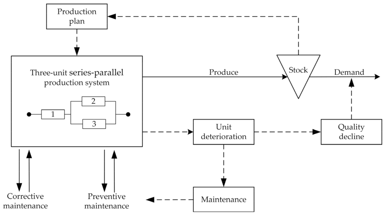
2. Problem Description and Assumptions

To better describe the joint optimization strategy, this section is divided into four parts. First of all, the research problem is described. Secondly, hypotheses are proposed for the research system. In the third part, the steady-state probability density function considering the structural relationship between units is described. Finally, unit deterioration in the production process impacts product quality and is reflected in the demand rate. The numerical relationship expression between the system state and demand rate is established.

2.1. Problem Description

The proposed system is a three-unit series–parallel production system that integrates batch production and preventive maintenance. The system produces only one kind of product. Our goal is to develop a reasonable production and maintenance model for the three-unit series–parallel production system to ensure the lowest cost rate by analyzing the various costs existing in the cycle. The decision variables are the production lot size and the preventive maintenance threshold of each unit.

Each unit in the proposed production system is in a new state at the initial production. With the progress of production, each unit has different degrees of deterioration. The deterioration process is represented by a gamma distribution, widely used for maintenance modeling [34]. Due to the deterioration of the system, a reasonable arrangement of unit maintenance actions can ensure the efficient work of the production system. Detection and maintenance activities are carried out at the end of production. The corresponding maintenance operation is required when the unit state detection reaches the threshold. For example, preventive maintenance operations are required when the state of unit 1 is greater than or equal to the preventive maintenance threshold at detection, and failure maintenance is required when the state is greater than or equal to the failure threshold. Normally, the cost of failure maintenance is much higher than preventive maintenance. In order to reduce the amount of failure maintenance, preventive maintenance should be increased, but excessive preventive maintenance will waste resources and increase costs. Therefore, it is necessary to set a reasonable preventive maintenance threshold. Each unit has different states at the end of the cycle, and the unit of the system is not a simple series relationship in reality. Some unnecessary units even exceed the failure threshold but do not affect the normal operation of the system. This paper studies the joint optimization of production and maintenance of a three-unit system with a series–parallel relationship. The relationship between units will determine whether the system can run normally, and the state of each unit will determine the maintenance operation at the end of the cycle. If the structural relationship between units is not taken into account, some unnecessary maintenance will be likely to happen. With the decline of the equipment state, the quality of the product decreases, and the proportion of low-quality products increases, which ultimately affects the demand rate. If the actual demand rate is lower than the maximum demand rate for a long time, excess production will occur. Considering the impact of the system state on the demand rate can better serve to formulate the production plan. The internal relationship diagram of the production system is shown in Figure 1. The relevant parameters and explanations are shown in

Table 1. Parameters and explanation.

Parameters	Explanation
Q	Economic production quantity, decision variable
$x_i$	State of unit $i$
$D_p^{(i)}$	Preventive maintenance threshold of unit $i$, decision variable
$D_f^{(i)}$	Failure threshold of unit $i$
$p_r$	Production rate of the system
$d_r$	Demand rate of the system
${\theta }_1$	The ratio of low-quality products in qualified products
${\theta }_2$	The ratio of repairable products in unqualified products
$c_{Set}$	The setting cost of single maintenance
$c_I$	Inventory cost per unit product
$c_R$	Repair cost per unit product
$c_S$	Shortage cost per unit time
$c_P$	Punishment cost
$c_{PM}^{(i)}$	Preventive maintenance cost of unit $i$
$c_{CM}^{(i)}$	Corrective maintenance cost of unit $i$
$g_1^{(i)}(t_{pm})$	The probability density function of PM time $t_{pm}$ of unit $i$
$g_2^{(i)}(t_{\mathrm{c}m})$	The probability density function of CM time $t_{\mathrm{c}m}$ of unit $i$

.

2.2. Assumptions

• Demand is periodic, production is continuous, and the production rate is always higher than the demand rate in the production cycle;
• Demand rate is variable, only related to product quality, and unchanged in one cycle;
• A part of the unqualified products can be repaired and completed instantly. The repaired part is all low-quality qualified products, and the unrepairable products are disposed after the end of the cycle;
• The production equipment has no sudden failure, and the equipment state is as new after maintenance;
• If multiple maintenance operations are carried out simultaneously, the setting cost is set only once [35];
• Only consider a single repair technician. That is to say, when the maintenance activities are carried out simultaneously or separately, the total maintenance time remains unchanged [20];
• The system can meet production requirements when the system does not need maintenance.

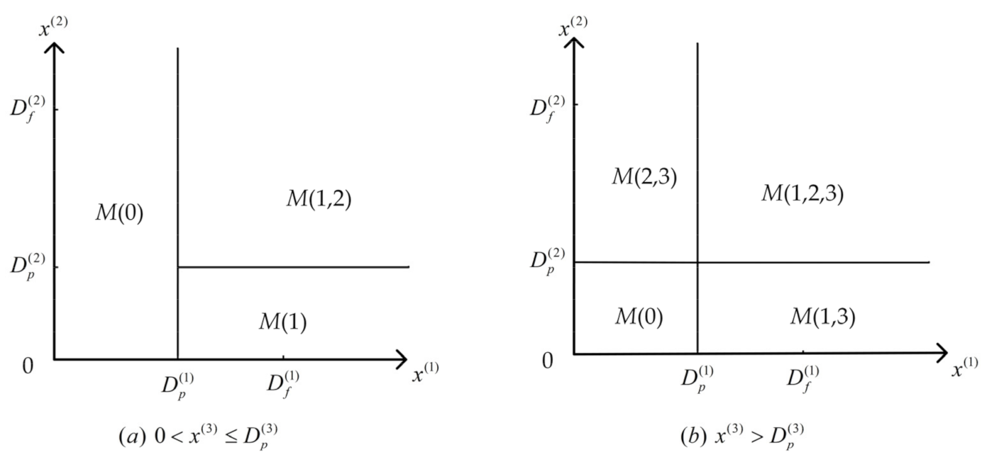
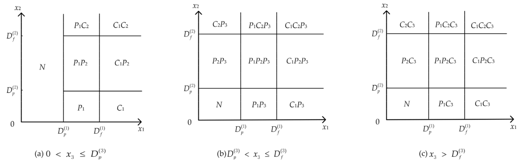
2.3. Steady-State Probability Density Function

According to the series–parallel production system shown in Figure 1, whether each unit needs maintenance is considered by using the DSSP method [24]. The division results are shown in Figure 2. For a piece of production equipment, the key components are different, and the threshold of each unit described in Figure 2 is different. The deterioration state space is divided into six maintenance groups according to Figure 2. (1) M (0) represents that no unit needs maintenance. (2) M (1) represents that only unit 1 needs maintenance. (3) M (1,2) represents that unit 1 and unit 2 need maintenance. (4) M (1,3) represents that unit 1 and unit 3 need maintenance. (5) M (2,3) represents that unit 2 and unit 3 need maintenance. (6) M (1,2,3) represents that unit 1, unit 2, and unit 3 need maintenance. Since each unit has different importance in the equipment, the maintenance combination of only maintenance unit 2 and only maintenance unit 3 does not exist.

It is assumed that the deterioration of each unit follows a gamma distribution. That is, the deterioration increment $\Delta x$ between two consecutive time units of unit $t$ follows $\mathrm{\Gamma }({\alpha }_i,{\beta }_i)$, and the increment $\Delta x^t$ of $t$ units of time follows $\mathrm{\Gamma }({\alpha }_{i}t,{\beta }_i)$ [24]. The probability density function can be expressed as:

$$f_i(x)=\frac{{\beta }^{{\alpha }_{i}t}{x}^{{\alpha }_{i}t-1}{e}^{-{\beta }_{i}x}}{\mathrm{\Gamma }({\alpha }_{i}t)},x>0$$

(1)

Each unit in the device has a state transition, as shown in Figure 3. When unit $i$ was maintained in the previous cycle, the initial state of the cycle is 0. When unit $i$ was not maintained in the previous cycle, the initial state of the cycle is $y_i$. After a period of deterioration, the state of unit $i$ is $x_i$.

Combined with the above six maintenance groups and Figure 3, the probability of different maintenance groups and the probability of state deterioration to $(x_1,x_2,x_3)$ are obtained, as shown in

Table 2. The probability of maintenance groups.

Maintenance Group Number	Probability of Maintenance Group	Deterioration Probability of Component State
(1) M (0)	$\begin{array}{l}{\displaystyle {\int }_0^{\min (x_1,D_p^{(1)})}{\displaystyle {\int }_0^{\infty }{\displaystyle {\int }_0^{\min (x_3,D_p^{(3)})}s(Y)d{y}_{1}d{y}_{2}d{y}_3}}}\\ +{\displaystyle {\int }_0^{\min (x_1,D_p^{(1)})}{\displaystyle {\int }_0^{\min (x_2,D_p^{(2)})}{\displaystyle {\int }_{D_p^{(3)}}^{\infty }s(Y)d{y}_{1}d{y}_{2}d{y}_3}}}\end{array}$	$f_1(x_1-y_1)f_2(x_2-y_2)f_3(x_3-y_3)$
(2) M (1)	${\displaystyle {\int }_{D_p^{(1)}}^{\infty }{\displaystyle {\int }_0^{\min (x_2,D_p^{(2)})}{\displaystyle {\int }_0^{\min (x_3,D_p^{(3)})}s(Y)d{y}_{1}d{y}_{2}d{y}_3}}}$	$f_1(x_1)f_2(x_2-y_2)f_3(x_3-y_3)$
(3) M (1,2)	${\displaystyle {\int }_{D_p^{(1)}}^{\infty }{\displaystyle {\int }_{D_p^{(2)}}^{\infty }{\displaystyle {\int }_0^{\min (x_3,D_p^{(3)})}s(Y)d{y}_{1}d{y}_{2}d{y}_3}}}$	$f_1(x_1)f_2(x_2)f_3(x_3-y_3)$
(4) M (1,3)	${\displaystyle {\int }_{D_p^{(1)}}^{\infty }{\displaystyle {\int }_0^{\min (x_2,D_p^{(2)})}{\displaystyle {\int }_{D_p^{(3)}}^{\infty }s(Y)d{y}_{1}d{y}_{2}d{y}_3}}}$	$f_1(x_1)f_2(x_2-y_2)f_3(x_3)$
(5) M (2,3)	${\displaystyle {\int }_0^{\min (x_1,D_p^{(1)})}{\displaystyle {\int }_{D_p^{(2)}}^{\infty }{\displaystyle {\int }_{D_p^{(3)}}^{\infty }s(Y)d{y}_{1}d{y}_{2}d{y}_3}}}$	$f_1(x_1-y_1)f_2(x_2)f_3(x_3)$
(6) M (1,2,3)	${\displaystyle {\int }_{D_p^{(1)}}^{\infty }{\displaystyle {\int }_{D_p^{(2)}}^{\infty }{\displaystyle {\int }_{D_p^{(3)}}^{\infty }s(Y)d{y}_{1}d{y}_{2}d{y}_3}}}$	$f_1(x_1)f_2(x_2)f_3(x_3)$

. The probability density function of the joint distribution of system state $s(x_1,x_2,x_3)$ is simplified to $s(X)$. $Y=(y_1,y_2,y_3)$ and $s(Y)$ represent the steady-state probability density function.

According to Table 2, the steady-state probability density function expression of the system can be described as follows:

$$\begin{array}{ll}s(Y)& ={\displaystyle {\int }_0^{\min (x_1,D_p^{(1)})}{\displaystyle {\int }_0^{\infty }{\displaystyle {\int }_0^{\min (x_3,D_p^{(3)})}s(Y)f_1(x_1-y_1)f_2(x_2-y_2)f_3(x_3-y_3)d{y}_{1}d{y}_{2}d{y}_3}}}\\ & +{\displaystyle {\int }_0^{\min (x_1,D_p^{(1)})}{\displaystyle {\int }_0^{\min (x_2,D_p^{(2)})}{\displaystyle {\int }_{D_p^{(3)}}^{\infty }s(Y)f_1(x_1-y_1)f_2(x_2-y_2)f_3(x_3-y_3)d{y}_{1}d{y}_{2}d{y}_3}}}\\ & +f_1(x_1){\displaystyle {\int }_{D_p^{(1)}}^{\infty }{\displaystyle {\int }_0^{\min (x_2,D_p^{(2)})}{\displaystyle {\int }_0^{\min (x_3,D_p^{(3)})}s(Y)f_2(x_2-y_2)f_3(x_3-y_3)d{y}_{1}d{y}_{2}d{y}_3}}}\\ & +f_1(x_1)f_2(x_2){\displaystyle {\int }_{D_p^{(1)}}^{\infty }{\displaystyle {\int }_{D_p^{(2)}}^{\infty }{\displaystyle {\int }_0^{\min (x_3,D_p^{(3)})}s(Y)f_3(x_3-y_3)d{y}_{1}d{y}_{2}d{y}_3}}}\\ & +f_1(x_1)f_3(x_3){\displaystyle {\int }_{D_p^{(1)}}^{\infty }{\displaystyle {\int }_0^{\min (x_2,D_p^{(2)})}{\displaystyle {\int }_{D_p^{(3)}}^{\infty }s(Y)f_2(x_2-y_2)d{y}_{1}d{y}_{2}d{y}_3}}}\\ & +f_2(x_2)f_3(x_3){\displaystyle {\int }_0^{\min (x_1,D_p^{(1)})}{\displaystyle {\int }_{D_p^{(2)}}^{\infty }{\displaystyle {\int }_{D_p^{(3)}}^{\infty }s(Y)f_1(x_1-y_1)d{y}_{1}d{y}_{2}d{y}_3}}}\\ & +f_1(x_1)f_2(x_2)f_3(x_3){\displaystyle {\int }_{D_p^{(1)}}^{\infty }{\displaystyle {\int }_{D_p^{(2)}}^{\infty }{\displaystyle {\int }_{D_p^{(3)}}^{\infty }s(Y)d{y}_{1}d{y}_{2}d{y}_3}}}\end{array}$$

(2)

2.4. Quality-Contingent Demand

With the progress of production, the equipment state change affects the quality of products. When the equipment state is worse, the defective rate of the product is higher, and the relationship between them is as shown in Equation (3) [36]. When the defective rate increases, considering product repair, the ratio of low-quality products increases, and the demand rate decreases. The relationship between the demand rate and the ratio of low-quality products is shown in Equation (4) [31].

$$p(x)=p_0+\eta (1-\exp (-\alpha x^{\beta }))$$

(3)

$$d_r=d_{\max }\times (1-\mu \times \rho )$$

(4)

where $p_0$ is the defective rate when the equipment is completely new, $\eta$ is the boundary of quality deterioration, $\alpha$ and $\beta$ are parameters obtained according to historical data, $d_{\max }$ represents the demand rate when all products are high-quality products, $\mu$ is the mediation coefficient, $0<\mu \le 1$, and $\rho$ is the low-quality qualified product rate in a production cycle, that is, the proportion of low-quality qualified products in the total number of products.

There are two types of low-quality products in a cycle; one is a certain proportion of low-quality products in qualified products, and the other is that unqualified products can be repaired and become low-quality products. The quantity calculation of these two kinds of low-quality products is shown in Equations (5) and (6). Since the proposed equipment is three-unit, ${\displaystyle {\int }_0^{t_n}p(x)}dt$ represents the defective rate of the system from 0 to $t_n$.

• The number of low-quality qualified products in qualified products is:

  $$N_1={\theta }_1\times Q\times (1-{\displaystyle {\int }_0^{t_n}p(x)}dt)$$

  (5)
• The number of low-quality qualified products repaired by unqualified products is:

  $$N_2={\theta }_2\times Q\times {\displaystyle {\int }_0^{t_n}p(x)}dt$$

  (6)

According to Equations (5) and (6), the ratio of low-quality qualified products in a production cycle is:

$$\rho =\frac{N_1+N_2}{Q}$$

(7)

Combining Equations (4) and (7), the demand rate can be obtained as follows:

$$d_r=d_{\max }\times (1-\mu \times ({\theta }_1\times (1-{\displaystyle {\int }_0^{t_n}p(x)}dt)+{\theta }_2\times {\displaystyle {\int }_0^{t_n}p(x)}dt))$$

(8)

3. Model Description

3.1. Production Description

The production rate of the system is $p_r$, and the demand rate $d_r$ remains constant in a cycle. The product lot size in one cycle is $Q$, and the production time is $t_n$, that is, $Q=p_r\times t_n$. At the end of each production cycle, each unit in the system is tested to determine the state and arrange reasonable maintenance activities. For each unit, corresponding maintenance is required when the state reaches the specified threshold. When the system is shut down for maintenance, the external demand is provided by the inventory. However, when the maintenance time is too long, the shortage cost exits. The possible inventory situation is shown in Figure 4.

According to Figure 4 and the production process, the maximum inventory $I_{\max }$ is described as follows:

$$I_{\max }=\frac{Q}{p_r}(p_r-d_r)$$

(9)

Maintenance time is a random variable, and it is assumed that there is only one repair technician. The shortage time of preventive maintenance alone $t_{spm}^{(1)}$ or corrective maintenance alone $t_{scm}^{(1)}$ of unit 1 can be calculated as Equations (10) and (11).

$$t_{spm}^{(1)}={\displaystyle {\int }_{\frac{Q(p_r-d_r)}{p_r{d}_r}}^{\infty }(t_{pm}-\frac{Q(p_r-d_r)}{p_r{d}_r})}{g}_1^{(1)}(t_{pm})d{t}_{pm}$$

(10)

$$t_{scm}^{(1)}={\displaystyle {\int }_{\frac{Q(p_r-d_r)}{p_r{d}_r}}^{\infty }(t_{cm}-\frac{Q(p_r-d_r)}{p_r{d}_r})}{g}_2^{(1)}(t_{cm})d{t}_{cm}$$

(11)

The corresponding maintenance time of unit 2 and unit 3 can be obtained by the same process. Then, $t_{spm}^{(2)}$, $t_{spm}^{(3)}$, $t_{scm}^{(2)}$, $t_{scm}^{(3)}$ can be calculated.

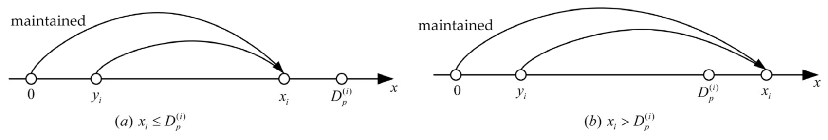
3.2. Maintenance Situation Description

To reduce the probability of equipment failure in the production process, each unit of the system is detected at the end of each production lot size $Q$. The appropriate maintenance strategy is determined according to the unit state and the structural characteristics of the unit. In the proposed system, due to the parallel relationship between unit 2 and unit 3, when only unit 2 or unit 3 fails, the whole system is still in regular operation at this time, and there is no need for a maintenance operation. Considering different operations at the end of the cycle, the system has the following twenty-three situations shown in Figure 5. In Figure 5, $N$ represents no maintenance, $P$ represents preventive maintenance, $C$ represents corrective maintenance, and the subscript $i$ represents unit $i$. For example, $P_1{C}_2$ represents that unit 1 needs preventive maintenance, unit 2 needs corrective maintenance, and unit 3 does not need maintenance.

According to Figure 5, the probability of each maintenance situation can be calculated. For example, the situation $N$ contains three areas. The first is $\left\{(x_1,x_2,x_3)\left|x_1\in \left[0,D_p^{(1)}\right),\right.x_2\in \left(0,\infty \right),x_3\in \left[0,D_p^{(3)}\right)\right\}$, in which the system can maintain regular work and does not need maintenance regardless of the state of unit 2. The second is $\left\{(x_1,x_2,x_3)\left|x_1\in \left[0,D_p^{(1)}\right),\right.x_2\in \left[0,D_p^{(2)}\right),x_3\in \left[D_p^{(3)},D_f^{(3)}\right)\right\}$, in which the system is regular even if the state of unit 3 exceeds the preventive maintenance threshold. Similarly, the third is $\left\{(x_1,x_2,x_3)\left|x_1\in \left[0,D_p^{(1)}\right),\right.x_2\in \left[0,D_p^{(2)}\right),x_3\in \left(D_f^{(3)},\infty \right)\right\}$. Its probability is described as

$$p(N)={\displaystyle {\int }_0^{D_p^{(1)}}{\displaystyle {\int }_0^{\infty }{\displaystyle {\int }_0^{D_p^{(3)}}s(X)}}}d{x}_{1}d{x}_{2}d{x}_3+{\displaystyle {\int }_0^{D_p^{(1)}}{\displaystyle {\int }_0^{D_p^{(2)}}{\displaystyle {\int }_{D_p^{(3)}}^{D_f^{(3)}}s(X)}}}d{x}_{1}d{x}_{2}d{x}_3+{\displaystyle {\int }_0^{D_p^{(1)}}{\displaystyle {\int }_0^{D_p^{(2)}}{\displaystyle {\int }_{D_f^{(3)}}^{\infty }s(X)}}}d{x}_{1}d{x}_{2}d{x}_3.$$

(12)

Similar to Equation (12), the probability of each situation can be calculated to prepare for modeling.

4. Model Formulation

According to the above description of the production and maintenance process, the model is established with the minimum expected cost rate. The expected cost rate in infinite time can be expressed as the expected cost rate in a single renewal cycle, according to renewal reward theory [37].

$$EC=E{C}_{\infty }=\frac{expected cost of a renewal cycle}{expected time of a renewal cycle}=\frac{E(C)}{E(T)}$$

(13)

The expected cost of a renewal cycle is the sum of the expected cost of all possible events multiplied by their corresponding probabilities, as shown in Equation (13). The definition of expected time is the same. According to Figure 5, there are 23 different situations, simplified as event $A_1,A_2,\cdots ,A_k,\cdots ,A_n$, and event $A_1,A_2,\cdots ,A_k,\cdots ,A_n$ forms all possible complete maintenance events in a renewal cycle with positive probability. Suppose event $A_1$ represents that the system does not need maintenance and $A_1=A_{11}\cup A_{12}$, where $A_{11}$ represents that the one of unit 2 or unit 3 fails. The expected cost can be described as Equation (14), and the expected time $E(T)$ can be described using the same method.

$$E(C)=E(C\left|A_1\right.)p(A_1)+E(C\left|A_2\right.)p(A_2)+\cdots +E(C\left|A_n\right.)p(A_n)$$

(14)

The probability of each situation can be obtained as Equation (12). Combining Equations (13) and (14), the expected cost rate in a renewal cycle can be described as

$$EC=\frac{E(C\left|A_{11}\right.)p(A_{11})+E(C\left|A_{12}\right.)p(A_{12})+E(C\left|A_2\right.)p(A_2)+\cdots +E(C\left|A_n\right.)p(A_n)}{E(T\left|A_1\right.)p(A_1)+E(T\left|A_2\right.)p(A_2)+\cdots +E(T\left|A_n\right.)p(A_n)}$$

(15)

4.1. Cost in a Renewal Cycle

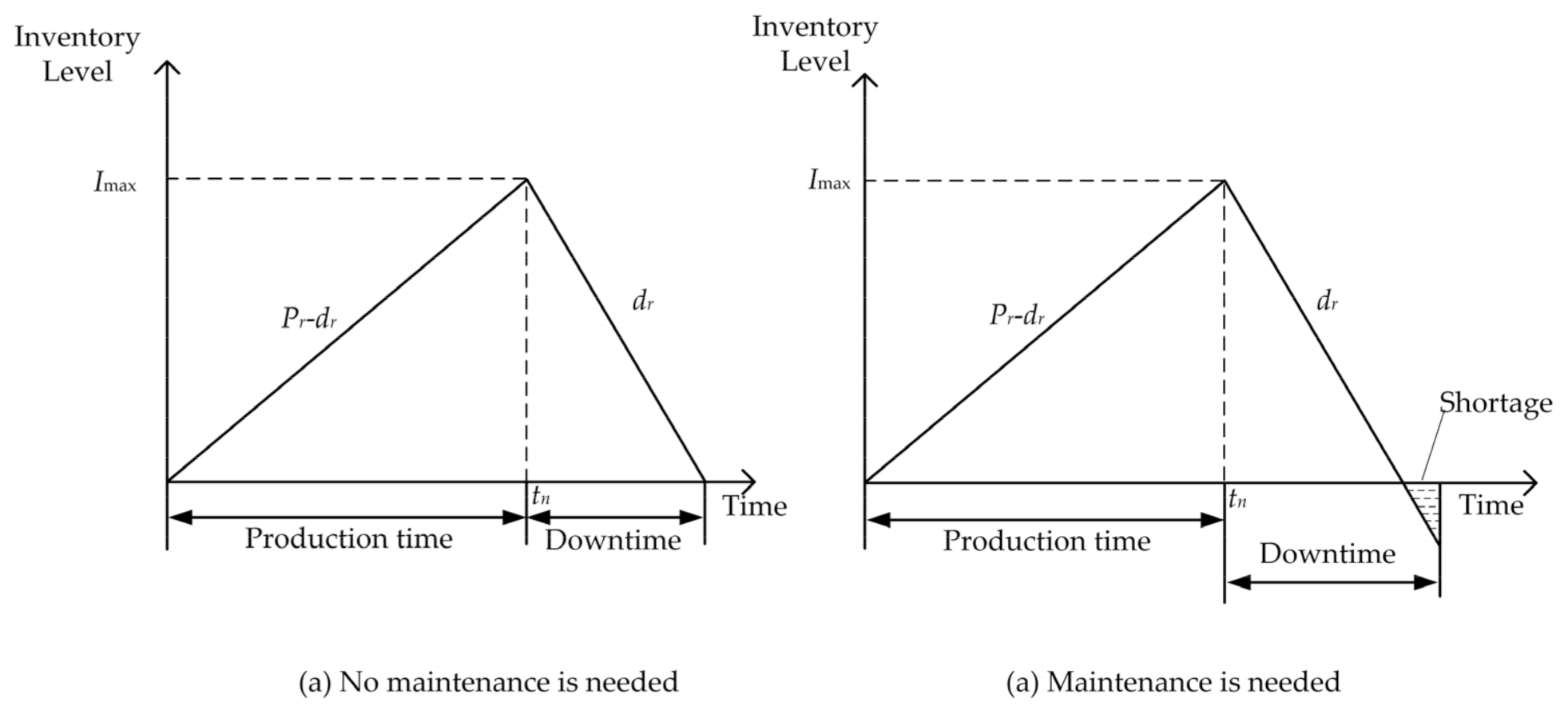
The proposed system describes the joint optimization problem of production and maintenance, taking into account possible costs, including setting cost $C_{Set}$, inventory cost $C_I$, repair cost $C_R$, shortage cost $C_S$, punishment cost $C_P$, preventive maintenance cost $C_{PM}$, and corrective maintenance cost $C_{CM}$. The setting cost $c_{Set}$ is a constant. For any maintenance event $A_k$, let $U_{PM}(A_k)$ be the set of preventive maintenance units and $U_{CM}(A_k)$ be the set of corrective maintenance units. Figure 5 shows the state of each unit when the system does not need maintenance. The punishment cost $c_P$ exists when unit 2 or unit 3 exceeds the failure threshold, and the system does not need maintenance. In this case, although the system has no fault, unit 2 or unit 3 fails, and another unit without faults in parallel may need to undertake additional work, which may cause losses. The existing costs are calculated below.

• inventory cost $C_I$
  According to the change of inventory level in the cycle described in Figure 4, the expected inventory level in a cycle can be represented by the area of the triangle in the inventory graph. The inventory cost $C_I$ can be described as

  $$C_I=c_I\times \frac{Q^2(p_r-d_r)}{2p_r{d}_r}$$

  (16)
• repair cost $C_R$
  The number of repairable unqualified products is obtained by Equation (6), and the repair cost can be described as

  $$C_R=c_R\times {\theta }_2\times Q\times {\displaystyle {\int }_0^{t_n}p(x)}dt$$

  (17)
• shortage cost $C_S$
  The shortage cost is generated only when the system is maintained, and it is related to the maintenance time. The calculation is divided into two parts. The first is that the shortage occurs when the system needs preventive maintenance, and the other is when the system needs corrective maintenance. The shortage time is shown as Equations (13) and (14), and the shortage cost $C_S$ of event $A_k$ can be described as

  $$C_S(A_k)=c_S\times d_r\times ({\displaystyle \sum _{i\in U_{PM}(A_k)}{t}_{spm}^{(i)}}+{\displaystyle \sum _{i\in U_{CM}(A_k)}{t}_{scm}^{(i)}})$$

  (18)
• Only when the one of unit 2 or unit 3 exceeds failure threshold does the punishment cost exists. The punishment cost $C_P$ of event $A_k$:

  $$C_P(A_k)=\left\{\begin{array}{l}{c}_P,A_k=A_{11}\\ 0,else\end{array}\right.$$

  (19)
• Preventive maintenance cost $C_{PM}$ of event $A_k$:

  $$C_{PM}(A_k)={\displaystyle \sum _{i\in U_{PM}(A_k)}{c}_{PM}^{(i)}}$$

  (20)
• Corrective maintenance cost $C_{CM}$ of event $A_k$:

  $$C_{CM}(A_k)={\displaystyle \sum _{i\in U_{CM}(A_k)}{c}_{CM}^{(i)}}$$

  (21)

The expected cost of event $A_k$ can be described as:

$$E(C\left|A_k\right.)=c_{Set}+C_I+C_R+C_S(A_k)+C_p(A_k)+C_{PM}(A_k)+C_{CM}(A_k)$$

(22)

4.2. Time in a Renewal Cycle

The expected time of a production cycle consists of production inventory consumption time and shortage time.

• Inventory consumption time:

  $$T_C=\frac{Q}{d_r}$$

  (23)
• Shortage time of event $A_k$:

  $$T_S(A_k)={\displaystyle \sum _{i\in U_{PM}(A_k)}{t}_{spm}^{(i)}}+{\displaystyle \sum _{i\in U_{CM}(A_k)}{t}_{scm}^{(i)}}$$

  (24)

The expected time of event $A_k$ can be described as:

$$E(T\left|A_k\right.)=T_C+T_S(A_k)$$

(25)

The process of calculating the probability of occurrence of event $A_k$ is similar to Equation (12). According to Equations (12)–(25), the model with the minimum system expected cost rate as the objective function is established.

$$\min EC(Q,D_p^{(i)})=\frac{E(C)}{E(T)}$$

(26)

$$subject to\left\{\begin{array}{l}0<D_p^{(i)}<D_f^{(i)}\\ d_r\le d_{\max }\\ d_r<p_r\\ Q\in N^{*}\end{array}\right.$$

(27)

where $Q$ and $D_p^{(i)}$ are decision variables to determine the optimal production lot size $Q^{*}$ of the system and the preventive maintenance threshold $D_p^{(i)}{}^{*}$ of each unit. The relationship between each unit threshold is restricted; that is, the preventive maintenance threshold $D_p^{(i)}$ of each unit is between 0 and the corrective maintenance threshold $D_f^{(i)}$. Restricted demand rate $d_r$ less than maximum demand rate $d_{\max }$ is based on Equation (8), and the demand rate $d_r$ less than the production rate $p_r$ is to ensure regular production. The lot size $Q$ must be a positive integer to ensure product integrity.

5. Resolution Method

This section is described from the steady-state probability density function solution method and the proposed model solution method.

5.1. Solution Method of Steady-State Probability Density Function

The value at the integral point can be obtained as Equation (29) by applying the approximate quadrature rule of Equation (28) to Equation (2). In the numerical calculation, $D_{\max }$ is used to replace $\infty$ in the Equation (29), so that $h_1=D_{\max }^{(1)}/i_{\max }$, $h_2$, $h_3$ can be obtained similarly.

$${\displaystyle {\int }_a^{b}y(s)ds={\displaystyle \sum _{j=1}^N{w}_{j}y(s_j)}}$$

(28)

$$\begin{array}{ll}\mathit{s}(i_1{h}_1,i_2{h}_2,i_3{h}_3)& =f_1(i_1{h}_1)f_2(i_2{h}_2)f_3(i_3{h}_3)-h_1{h}_2{h}_3{\displaystyle \sum _{j_1=m_1}^{i_{\max }}{\displaystyle \sum _{j_2=m_2}^{i_{\max }}{\displaystyle \sum _{j_3=1}^{m_3}\mathit{s}(i_1{h}_1,i_2{h}_2,i_3{h}_3)f_1(i_1{h}_1)f_2(i_2{h}_2)f_3(i_3{h}_3)}}}\\ & +h_1{h}_2{h}_3{\displaystyle \sum _{j_1=1}^{\min (i_1,m_1)}{\displaystyle \sum _{j_2=1}^{i_{\max }}{\displaystyle \sum _{j_3=1}^{\min (i_3,m_3)}\mathit{s}(i_1{h}_1,i_2{h}_2,i_3{h}_3)f_1(i_1{h}_1-j_1{h}_1)f_2(i_2{h}_2-j_2{h}_2)f_3(i_3{h}_3-j_3{h}_3)}}}\\ & +h_1{h}_2{h}_3{\displaystyle \sum _{j_1=1}^{\min (i_1,m_1)}{\displaystyle \sum _{j_2=1}^{\min (i_2,m_2)}{\displaystyle \sum _{j_3=m_3}^{i_{\max }}\mathit{s}(i_1{h}_1,i_2{h}_2,i_3{h}_3)f_1(i_1{h}_1-j_1{h}_1)f_2(i_2{h}_2-j_2{h}_2)f_3(i_3{h}_3-j_3{h}_3)}}}\\ & +h_1{h}_2{h}_3{\displaystyle \sum _{j_1=m_1}^{i_{\max }}{\displaystyle \sum _{j_2=1}^{\min (i_2,m_2)}{\displaystyle \sum _{j_3=1}^{\min (i_3,m_3)}\mathit{s}}}}(i_1{h}_1,i_2{h}_2,i_3{h}_3)f_1(i_1{h}_1)f_2(i_2{h}_2-j_2{h}_2)f_3(i_3{h}_3-j_3{h}_3)\\ & +h_1{h}_2{h}_3{\displaystyle \sum _{j_1=m_1}^{i_{\max }}{\displaystyle \sum _{j_2=m_2}^{i_{\max }}{\displaystyle \sum _{j_3=1}^{\min (i_3,m_3)}\mathit{s}}}}(i_1{h}_1,i_2{h}_2,i_3{h}_3)f_1(i_1{h}_1)f_2(i_2{h}_2)f_3(i_3{h}_3-j_3{h}_3)\\ & +h_1{h}_2{h}_3{\displaystyle \sum _{j_1=m_1}^{i_{\max }}{\displaystyle \sum _{j_2=1}^{\min (i_2,m_2)}{\displaystyle \sum _{j_3=m_3}^{i_{\max }}\mathit{s}}}}(i_1{h}_1,i_2{h}_2,i_3{h}_3)f_1(i_1{h}_1)f_2(i_2{h}_2-j_2{h}_2)f_3(i_3{h}_3)\\ & +h_1{h}_2{h}_3{\displaystyle \sum _{j_1=1}^{\min (i_1,m_1)}{\displaystyle \sum _{j_2=m_2}^{i_{\max }}{\displaystyle \sum _{j_3=m_3}^{i_{\max }}\mathit{s}(i_1{h}_1,i_2{h}_2,i_3{h}_3)}}}{f}_1(i_1{h}_1-j_1{h}_1)f_2(i_2{h}_2)f_3(i_3{h}_3)\end{array}$$

(29)

Let $\mathit{s}=\mathit{s}(i_1{h}_1,i_2{h}_2,i_3{h}_3)$ be the three-dimensional array of solutions, $\mathit{f}$ be the array $\mathit{f}(i_1{h}_1,i_2{h}_2,i_3{h}_3)$. ${\mathit{K}}^i$ represents the three-dimensional array ${\mathit{K}}_{i_{\max }\times i_{\max }\times i_{\max }}^i$, and its definition is ${\mathit{K}}^i=h_1{h}_2{h}_3{\mathit{K}}^{i1}{\mathit{K}}^{i2}{\mathit{K}}^{i3}$, ${\mathit{K}}^{i1}={\left\{k_{i_1{j}_1}^{11}\right\}}_{i_{\max }\times i_{\max }},{\mathit{K}}^{i2}={\left\{k_{i_2{j}_2}^{12}\right\}}_{i_{\max }\times i_{\max }}$, ${\mathit{K}}^{i3}={\left\{k_{i_3{j}_3}^{13}\right\}}_{i_{\max }\times i_{\max }}$, $i=(1,2,\cdots ,7)$. Equation (29) is changed into the form of Equation (30), and the specific calculation of ${\mathit{K}}^i$ is shown in Appendix A.

$$(\mathit{I}{+\mathit{K}}^1-{\mathit{K}}^2-{\mathit{K}}^3-{\mathit{K}}^4-{\mathit{K}}^5-{\mathit{K}}^6-{\mathit{K}}^7)\mathit{s}=\mathit{f}$$

(30)

The steady-state probability density function can be obtained by solving the approximate numerical solution $\mathit{s}=\mathit{s}(i_1{h}_1,i_2{h}_2,i_3{h}_3)$ of the implicit equation.

5.2. Solution Method of the Proposed Model

Equation (26) shows four decision variables in the proposed model, and the solution space is enormous. The traditional calculation method is challenging to calculate, so the intelligent algorithm is selected for solving. Since the genetic algorithm performs well in solving the problem of ample solution space, the genetic algorithm is chosen. At the same time, the elite strategy can ensure that the optimal individual of each generation can be retained. In this paper, the worst individual is replaced by the optimal individual to ensure the evolution of the population. Since the genetic algorithm generally solves the maximum value problem, the objective function is taken as the inverse, that is, $fitness=-EC(Q,D_p^{(i)})$. In addition, the real number is used for coding in the algorithm. The real number coding linear crossover is applied in the crossover operation, and the roulette method with $fitness=fitness-\min (fitness)$ as input data is proposed to distinguish different fitness values in a select process better. The mutation probability $p_{mut}$ gradually decreases with a fixed attenuation coefficient $\delta$ to make the population gradually stable and obtain a better solution [30], that is, $p_{mut}=\delta \times p_{mut}$. The proposed genetic algorithm flow chart is shown in Figure 6.

6. Numerical Analysis

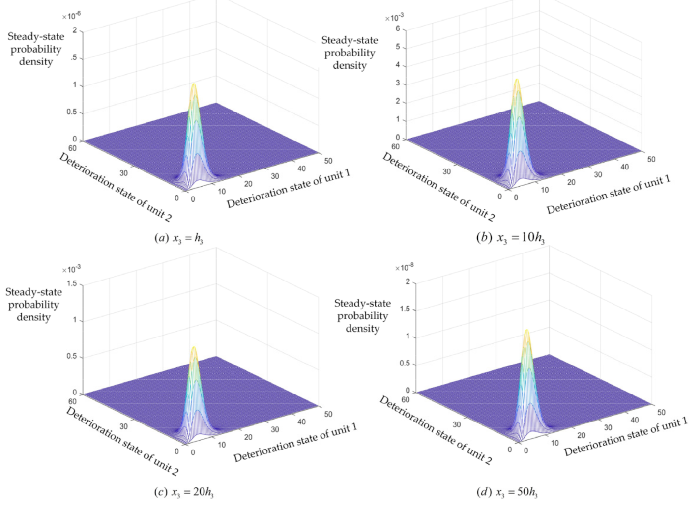
6.1. Verification of Steady-State Probability Density Function

As the steady-state probability density function of the deteriorating state, $s(X)$ should have the general characteristics of the probability density function, that is, the integral in the whole state space is 1. Let $r={\displaystyle {\int }_0^{\infty }{\displaystyle {\int }_0^{\infty }{\displaystyle {\int }_0^{\infty }s(X)}}}d{x}_{1}d{x}_{2}d{x}_3$.

Table 3. Value of r under different parameters.

Unit 1	Unit 2	Unit 3	$\mathit{r} {\mathit{i}}_{\mathbf{max}} = 25$	${\mathit{r}}^{\prime }{\mathit{i}}_{\mathbf{max}} = 50$	${\mathit{r}}^{″}{\mathit{i}}_{\mathbf{max}} = 100$
${\alpha }_1=2,{\beta }_1=1.5$	${\alpha }_2=1.5,{\beta }_2=0.8$	${\alpha }_3=1.5,{\beta }_3=0.8$	1.0043	1.0011	1.0003
${\alpha }_1=1.2,{\beta }_1=0.8$	${\alpha }_2=1,{\beta }_2=0.6$	${\alpha }_3=1,{\beta }_3=0.6$	1.0045	1.0012	1.0003
${\alpha }_1=1.2,{\beta }_1=2$	${\alpha }_2=2,{\beta }_2=2.5$	${\alpha }_3=2,{\beta }_3=2.5$	0.9737	1.0021	1.0007
${\alpha }_1=0.7,{\beta }_1=1.2$	${\alpha }_2=1.1,{\beta }_2=0.9$	${\alpha }_3=1.1,{\beta }_3=0.9$	1.0134	1.0026	1.0003
${\alpha }_1=0.7,{\beta }_1=2$	${\alpha }_2=0.9,{\beta }_2=1.5$	${\alpha }_3=0.9,{\beta }_3=1.5$	1.0231	1.0134	1.0014

shows the calculation results of different parameters, where $D_{\max }^{(i)}=5\times D_f^{(i)}$, $D_f^{(1)}=10$, $D_f^{(2)}=12$, $D_f^{(3)}=12$, $D_p^{(1)}=8$, $D_p^{(2)}=9.6$,$D_p^{(3)}=9.6$, and ${\alpha }_i$ and ${\beta }_i$ are the shape parameters and size parameters of the deterioration process of unit $i$, respectively. The larger the $i_{\max }$, the smaller the step size $h_i$, and the higher the accuracy, as shown in Table 3. No matter the $i_{\max }$, it can be found that the values are close to 1, which proves that the definition and numerical solution of the steady-state probability density function of the series–parallel three-unit system proposed are correct.

According to the approximate quadrature rule, the fourth data and $i_{\max }=100$ are selected to draw the approximate numerical solution of the steady-state probability density function diagram, as shown in Figure 7.

The data in Table 3 show that when the unit obeys the distribution functions with different parameters, the result of $r$ is always close to 1. At the same time, when the $i_{\max }$ is larger, the representation accuracy is closer to 1. However, the increase in accuracy will lead to a rise in calculation time. Therefore, the fourth group of data with $i_{\max }=100$ is selected to draw the approximate solution of the steady-state probability density function of the system. It can be seen from Figure 6 that when the maintenance threshold of the unit is determined, each unit has a maximum probability density, which conforms to the law of normal deterioration.

6.2. Case Study

The proposed system is a three-unit series–parallel system, as shown in Figure 1. The deterioration of unit $i$ follows a gamma distribution, and the shape and size parameters are ${\alpha }_i$ and ${\beta }_i$, respectively. The preventive maintenance time and corrective maintenance time of unit $i$ are exponentially distributed with parameters ${\lambda }_i$ and ${\mu }_i$, respectively. The maintenance-related parameters of each unit are shown in

Table 4. Parameters of units.

$\mathbf{Unit} \mathit{i}$	${\mathit{\alpha }}_{\mathit{i}}$	${\mathit{\beta }}_{\mathit{i}}$	${\mathit{D}}_{\mathit{f}}^{(\mathit{i})}$	${\mathit{c}}_{\mathit{P}\mathit{M}}^{(\mathit{i})}$	${\mathit{c}}_{\mathit{C}\mathit{M}}^{(\mathit{i})}$	${\mathit{\lambda }}_{\mathit{i}}$	${\mathit{\mu }}_{\mathit{i}}$
1	1.4	2.8	10	1600	4700	1	0.5
2	2.2	3.2	12	1400	4200	2	1
3	2.2	3.2	12	1400	4200	2	1

. In addition, the production and cost parameters considered in the proposed model are shown in

Table 5. Parameters of system.

Parameter	Value	Parameter	Value
$p_r$(unit/day)	200	$\beta$	1.26
$d_{\max }$(unit/day)	160	$\mu$	0.1
${\theta }_1$	0.1	$c_{Set}$ (Yuan/each time)	600
${\theta }_2$	0.6	$c_I$ (Yuan/unit/day)	0.5
$p_0$	0.004	$c_R$ (Yuan/unit)	10
$\eta$	0.071	$c_S$ (Yuan/unit)	20
$p_0$	0.0046	$c_P$ (Yuan)	1000

[30].

According to the solving process shown in Figure 6, the genetic algorithm parameters are set as follows: crossover probability $p_{cro}=0.8$, initial mutation probability $p_{mut}=0.1$, reduction coefficient $\delta =0.98$, population size $N=40$, and iteration number $L=50$. It should be noted that through the previous calculation, it can be known that the thresholds of unit 2 and unit 3 are roughly the same. Since unit 2 and unit 3 are two identical parallel units, their preventive maintenance thresholds are consistent. Thus, in the final encoding calculation, the two are set to be equal, and the operation is in line with the reality. The optimal strategy for 50 experiments is $EC(881,6.96,8.25,8.25)=217.5198$. For this enterprise, when the lot size is set to 881, the preventive maintenance threshold of unit 1 is 6.96, and the preventive maintenance thresholds of units 2 and 3 are 8.25, and the total cost rate of long-term production of the system is the lowest at 217.5198. The iteration diagram is shown in Figure 8.

6.3. Sensitivity Analysis

This section analyzes the impact on the results by changing the input parameters. Each calculation only varies the value of one parameter, ranging from −50% to +50%. Other parameters remain unchanged, and the changes in the results are observed. Since unit 2 and unit 3 are the same two units, their two parameters change simultaneously. Hereby, this part selects ${\theta }_1$, ${\theta }_2$, μ, $c_{Set}$, $c_I$, $c_R$, $c_S$, $c_P$, $c_{PM}^{(1)}$, $c_{PM}^{(2)}$, a total of 10 parameters for analysis. The influence of parameter changes on lot size $Q$, preventive maintenance threshold of unit 1 $D_p^{(1)}$, preventive maintenance threshold of unit 2 $D_p^{(2)}$, and expected cost rate $EC$ are shown in Figure 9.

Figure 9a shows the influence of parameter changes on the optimal production lot size $Q$. We can see that two parameters have significant effects on lot size. The first is the setting cost $c_{Set}$. With the increase of setting cost, the quantity has an apparent upward trend. When the setting cost increases, the PM thresholds $D_p^{(i)}$ increase to minimize the expected cost rate and reduce the frequency of maintenance operations. When the production time increases, the lot size increases significantly. The second is inventory cost $c_I$. When inventory cost increases, the production lot size is reduced to minimize the expected cost rate.

Figure 9b shows the influence of parameter changes on the preventive maintenance threshold of unit 1. $D_p^{(1)}$ is sensitive to the ten parameters analyzed. The most sensitive is setting cost $c_{Set}$ and PM cost of unit 2 $c_{PM}^{(2)}$. Similar to Figure 9a, when setting cost increases, the PM threshold $D_p^{(1)}$ increases to reduce maintenance frequency. When the PM cost of unit 2 increases, the threshold of unit 2 $D_p^{(2)}$ increases to reduce the frequency of maintenance unit 2, and $D_p^{(1)}$ decreases to decrease the expected cost rate.

Figure 9c shows the influence of parameter changes on the preventive maintenance threshold of unit 2. $D_p^{(2)}$ is similar to $D_p^{(1)}$. The most sensitive is setting cost $c_{Set}$ and PM cost of unit 1 $c_{PM}^{(1)}$. When setting cost increases, the PM threshold $D_p^{(2)}$ increases to reduce maintenance frequency. When the PM cost of unit 1 increases, the threshold of unit 2 $D_p^{(1)}$ increases to reduce the frequency of maintenance unit 1, and $D_p^{(2)}$ decreases to decrease the expected cost rate.

Figure 9d shows the impact of parameters on the expected cost rate. It can be seen from the figure that the expected cost rate is more sensitive to setting cost $c_{Set}$ and inventory cost $c_I$. This is because the increase in setting cost causes a lot of changes in the production lot size, resulting in an increase in inventory costs and thus affecting the expected cost rate. Overall, the expected cost rate is still increasing.

In the established context, different costs will affect the cost rate of the enterprise, affecting the decisions of decision-makers. Therefore, in the normal production process, considering the relationship between different units, it is useful to develop a reasonable and effective production and maintenance plan for the enterprise.

6.4. Contrast Experiment

This section sets up two contrast experiments. First, the influence of maintenance on the system probability density function is not considered. That is, the probability distribution function is handled according to the set function, and other conditions remain unchanged. The second is that the influence of the structure between units on the system is not considered. That is, the unit will perform relevant operations as long as it reaches the maintenance threshold.

• Maintenance policy is independent of system structure
  When the maintenance operation does not affect the probability density function of the system, the probability density function of the system $s^{\prime }(x_1,x_2,x_3)$ can be expressed as

  $$s^{\prime }(x_1,x_2,x_3)=f_1(x_1)f_2(x_2)f_3(x_3)$$

  (31)
  Other remaining settings remain unchanged. After 20 experiments, the optimal strategy is $EC(807,8.31,10.17,10.17)=217.6142$. Compared with the results of this paper, it can be found that there is little difference in the cost rate, but without considering the influence of maintenance on the unit, the optimal preventive maintenance threshold of the three units is significantly higher than the results of this paper. In the actual production process, it is very likely to reach the fault threshold in the production process, affecting the normal production process.
• System probability density function is not affected by the maintenance operation
  In this case, there will be 27 maintenance situations in the production process. Each unit has three maintenance situations, and there are $3\times 3\times 3=27$ maintenance situations in the system. Maintenance situations are as shown in Figure 10, and the representation method is the same in Figure 5.

According to the modeling idea, the situation is modeled and solved. The optimal strategy is $EC(880,6.91,8.39,8.39)=217.2128$. When the influence of the structural relationship between units on the maintenance combination is not considered, the expected cost rate is similar to the value of the model proposed in this paper. However, in theory, due to the failure of some non-key components, the overall shutdown maintenance of the system is required, which may lead to excessive system maintenance and waste of resources. At the same time, in the analysis of the expected cost rate, it is found that although the cost is reduced, the cycle becomes longer, which may lead to short supply or overtime.

Overall, the proposed model takes into account the specific situation in the real production system, which is more realistic and can guide the decision-making of enterprises.

7. Conclusions

This paper studies the joint optimization problem of production- and condition-based maintenance of a three-unit production system. The DSSP method is extended and applied to the three-unit series–parallel system, and the numerical solution of the steady-state probability density function is given. Under the condition that the market has strict quality requirements and a rapid response, the impact of product quality on demand is considered. The relationship between unit deterioration state and demand rate is given. In addition, the economic principle is considered for maintenance groupings between different units. The production and maintenance situations in one cycle are analyzed to establish the model. The proposed model takes the minimum expected cost rate as the objective function to determine the optimal production lot size and preventive maintenance threshold of each unit. According to the characteristics of the model, an improved genetic algorithm is designed. Finally, sensitivity analysis shows the influence of each parameter on decision-making, which is helpful for decision-making. The model can be applied to complex mass production systems, such as transistor manufacturing systems, consumables production systems, etc.

One limitation of this paper is that the research object is a three-unit system, and a system above three units needs to be further expanded. The dimension of the linear equations of the steady-state probability density function increases exponentially with the number of units, and the improved genetic algorithm may fall into the local optimum in the experiment. Therefore, finding more efficient equation solutions is conducive to the subsequent expansion of applications. In future work, we can relax some assumptions to make the model more realistic. For example, the unit returns to a better state after maintenance rather than when new. When a parallel unit fails, the deterioration of other units may accelerate, and the punishment cost can be calculated. In addition, the joint optimization can also be combined with the control chart to improve product quality and reduce cost rate.

References

1. Schreiber, M.; Vernickel, K.; Richter, C.; Reinhart, G. Integrated production and maintenance planning in cyber-physical production systems. Procedia CIRP 2019, 79, 534–539. [Google Scholar] [CrossRef]
2. Vogel, T.; Almada-Lobo, B.; Almeder, C. Integrated versus hierarchical approach to aggregate production planning and master production scheduling. OR Spectrum 2016, 39, 193–229. [Google Scholar] [CrossRef]
3. Rossi, T.; Pozzi, R.; Pero, M.; Cigolini, R. Improving production planning through finite-capacity MRP. Int. J. Prod. Res. 2017, 55, 377–391. [Google Scholar] [CrossRef]
4. Guo, Z.X.; Wong, W.K.; Zhi, L.; Ren, P. Modeling and Pareto optimization of multi-objective order scheduling problems in production planning. Comput. Ind. Eng. 2013, 64, 972–986. [Google Scholar] [CrossRef]
5. Hervert-Escobar, L.; López-Pérez, J.F. Production planning and scheduling optimization model: A case of study for a glass container company. Ann. Oper. Res. 2018, 286, 529–543. [Google Scholar] [CrossRef] [Green Version]
6. Andriolo, A.; Battini, D.; Persona, A.; Sgarbossa, F. A new bi-objective approach for including ergonomic principles into EOQ model. Int. J. Prod. Res. 2015, 54, 2610–2627. [Google Scholar] [CrossRef]
7. Massonnet, G.; Gayon, J.; Rapine, C. Approximation algorithms for deterministic continous-review inventory lot-sizing problems with time-varying demand. Eur. J. Oper. Res. 2014, 234, 641–649. [Google Scholar] [CrossRef]
8. Ou, J.; Feng, J. Production lot-sizing with dynamic capacity adjustment. Eur. J. Oper. Res. 2019, 272, 261–269. [Google Scholar] [CrossRef]
9. Lamas, A.; Chevalier, P. Joint dynamic pricing and lot-sizing under competition. Eur. J. Oper. Res. 2018, 266, 864–876. [Google Scholar] [CrossRef] [Green Version]
10. Makis, V.; Fung, J. An EMQ model with inspections and random machine failures. J. Oper. Res. Soc. 1998, 49, 66–76. [Google Scholar] [CrossRef]
11. Farahani, A.; Tohidi, H. Integrated optimization of quality and maintenance: A literature review. Comput. Ind. Eng. 2021, 151, 106924. [Google Scholar] [CrossRef]
12. Marquez, A.C.; Yin, X.; Liu, X. The Maintenance Management Framework: Models and Methods for Complex Systems Maintenance; National Defence Industry Press: Beijing, China, 2013; pp. 49–50. [Google Scholar]
13. Cassady, C.R.; Kutanoglu, E. Integrating preventive maintenance planning and production scheduling for a single machine. IEEE T. Reliab. 2005, 54, 304–309. [Google Scholar] [CrossRef]
14. Wang, C. Optimal production and maintenance policy for imperfect production systems. Nav. Res. Logist. 2006, 53, 151–156. [Google Scholar] [CrossRef]
15. Liao, G.; Sheu, S. Economic production quantity model for randomly failing production process with minimal repair and imperfect maintenance. Int. J. Prod. Econ. 2011, 130, 118–124. [Google Scholar] [CrossRef]
16. Zandieh, M.; Sajadi, S.M.; Behnoud, R. Integrated production scheduling and maintenance planning in a hybrid flow shop system: A multi-objective approach. Int. J. Syst. Assur. Eng. Manag. 2017, 8, 1630–1642. [Google Scholar] [CrossRef]
17. Zhang, X.; Xia, T.; Pan, E.; Li, Y. Integrated optimization on production scheduling and imperfect preventive maintenance considering multi-degradation and learning-forgetting effects. Flex. Serv. Manuf. J. 2022, 34, 451–482. [Google Scholar] [CrossRef]
18. Liao, W.; Chen, M.; Yang, X. Joint optimization of preventive maintenance and production scheduling for parallel machines system. J. Intell. Fuzzy Syst. 2017, 32, 913–923. [Google Scholar] [CrossRef]
19. Tian, Z.; Liao, H. Condition based maintenance optimization for multi-component systems using proportional hazards model. Reliab. Eng. Syst. Saf. 2011, 96, 581–589. [Google Scholar] [CrossRef]
20. Van, P.D.; Barros, A.; Bérenguer, C.; Bouvard, K.; Brissaud, F. Dynamic grouping maintenance with time limited opportunities. Reliab. Eng. Syst. Saf. 2013, 120, 51–59. [Google Scholar] [CrossRef]
21. Vu, H.C.; Do, P.; Barros, A. A Stationary Grouping Maintenance Strategy Using Mean Residual Life and the Birnbaum Importance Measure for Complex Structures. IEEE Trans. Reliab. 2016, 65, 217–234. [Google Scholar] [CrossRef]
22. Nguyen, K.; Do, P.; Grall, A. Condition-based maintenance for multi-component systems using importance measure and predictive information. Int. J. Syst. Sci. Oper. Logist. 2014, 1, 228–245. [Google Scholar] [CrossRef]
23. Cheng, G.; Zhou, B.; Li, L. Joint optimization of lot sizing and condition-based maintenance for multi-component production systems. Comput. Ind. Eng. 2017, 110, 538–549. [Google Scholar] [CrossRef]
24. Zhang, X.; Zeng, J. Deterioration state space partitioning method for opportunistic maintenance modelling of identical multi-unit systems. Int. J. Prod. Res. 2015, 53, 2100–2118. [Google Scholar] [CrossRef]
25. Zhang, X.; Zeng, J. Joint optimization of condition-based opportunistic maintenance and spare parts provisioning policy in multiunit systems. Eur. J. Oper. Res. 2017, 262, 479–498. [Google Scholar] [CrossRef]
26. Zhang, X.; Zeng, J.; Gan, J. Joint optimization of condition-based maintenance and spare part inventory for two-component system. J. Ind. Prod. Eng. 2018, 35, 394–420. [Google Scholar] [CrossRef]
27. Zhang, X.; Liao, H.; Zeng, J.; Shi, G.; Zhao, B. Optimal Condition-based Opportunistic Maintenance and Spare Parts Provisioning for a Two-unit System using a State Space Partitioning Approach. Reliab. Eng. Syst. Saf. 2021, 209, 107451. [Google Scholar] [CrossRef]
28. Gan, J.; Wang, L.; Zhang, X.; Zhang, W. The Joint Decision and Optimization of Single Machine Scheduling and Imperfect Condition Based Maintenance. Ind. Eng. Manag. 2021, 26, 75–81. [Google Scholar]
29. Zhang, X.; Zeng, J. Optimal maintenance modeling for systems with multiple non-identical units using extended DSSP method. Am. J. Oper. Res. 2016, 6, 275–295. [Google Scholar] [CrossRef] [Green Version]
30. Gao, Z.; Wang, H.; Zhang, H. The Decision of Production Systems with Quality-Contingent Demand and Condition-Based Maintenance. Systems 2022, 10, 20. [Google Scholar] [CrossRef]
31. Lu, Z.; Xue, J.; Yang, Y. The decision of economic production quantity with quality-contingent demand and perfect preventative maintenance. Chin. J. Manag. Sci. 2020, 28, 71–78. [Google Scholar]
32. Pasandideh, S.H.R.; Niaki, S.T.A. A genetic algorithm approach to optimize a multi-products EPQ model with discrete delivery orders and constrained space. Appl. Math. Comput. 2008, 195, 506–514. [Google Scholar] [CrossRef]
33. Pal, S.; Maiti, M.K.; Maiti, M. An EPQ model with price discounted promotional demand in an imprecise planning horizon via Genetic Algorithm. Comput. Ind. Eng. 2009, 57, 181–187. [Google Scholar] [CrossRef]
34. Noortwijk, J.M. A survey of the application of gamma processes in maintenance. Reliab. Eng. Syst. Saf. 2009, 94, 2–21. [Google Scholar] [CrossRef]
35. Castanier, B.; Grall, A.; Bérenguer, C. A condition-based maintenance policy with non-periodic inspections for a two-unit series system. Reliab. Eng. Syst. Saf. 2005, 87, 109–120. [Google Scholar] [CrossRef]
36. Bouslah, B.; Gharbi, A.; Pellerin, R. Integrated production, sampling quality control and maintenance of deteriorating production systems with AOQL constraint. Omega 2016, 61, 110–126. [Google Scholar] [CrossRef]
37. Grall, A.; Dieulle, L.; Berenguer, C.; Roussignol, M. Continuous-time predictive-maintenance scheduling for a deteriorating system. IEEE Trans. Reliab. 2002, 51, 141–150. [Google Scholar] [CrossRef] [Green Version]
Figure 1. The internal relationship of the proposed three-unit production system.
Applsci 12 07558 g001
Figure 2. Deterioration state partition diagram of three-unit series–parallel equipment.
Applsci 12 07558 g002
Figure 3. State transition diagram of unit i .
Applsci 12 07558 g003
Figure 4. Possible inventory situation.
Applsci 12 07558 g004
Figure 5. Division of maintenance situations.
Applsci 12 07558 g005
Figure 6. The proposed genetic algorithm flow chart.
Applsci 12 07558 g006
Figure 7. The approximate numerical solution of the steady-state probability density function of the joint state of the proposed system s ( x 1 , x 2 , x 3 ) .
Applsci 12 07558 g007
Figure 8. Iteration diagram.
Applsci 12 07558 g008
Figure 9. Influence of parameters.
Applsci 12 07558 g009
Figure 10. Division of maintenance situations without considering system structure.
Applsci 12 07558 g010