
Fv-AD: F-AnoGAN Based Anomaly Detection in Chromate Process for Smart Manufacturing


Abstract
:1. Introduction
2. Related Work
2.1. Anomaly Detection in Smart Factory
2.2. Unsupervised Learning for Anomaly Detection
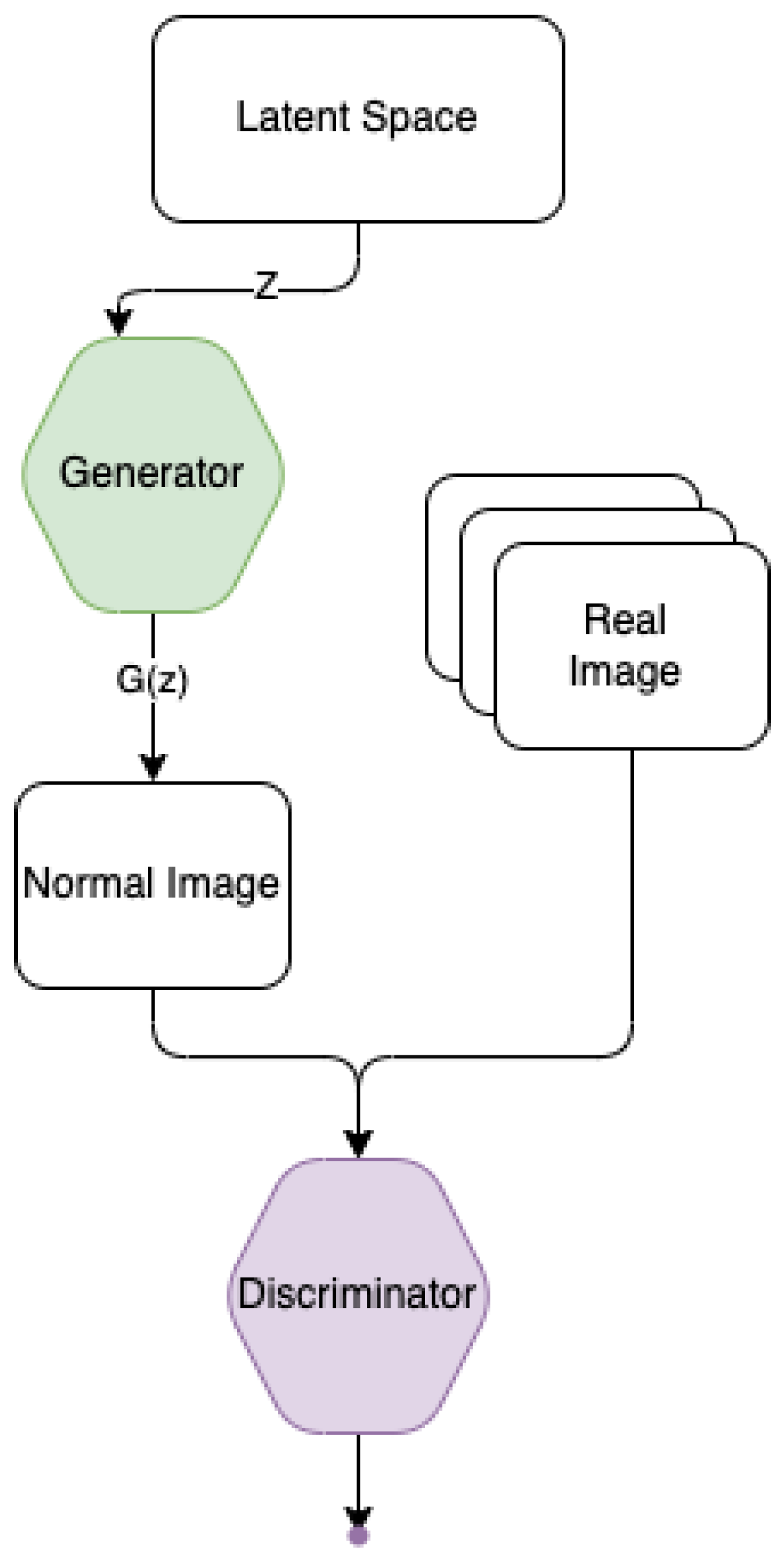
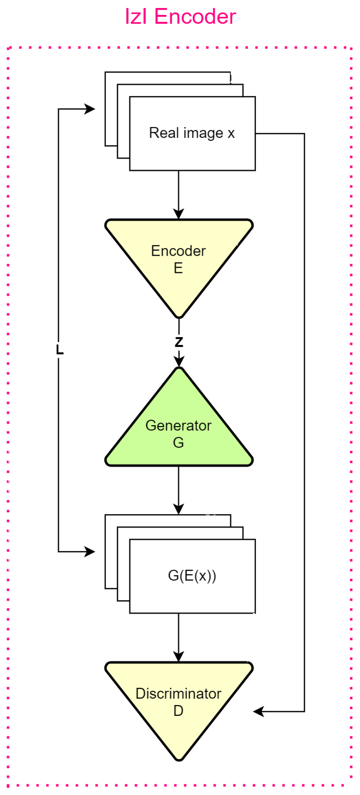
2.3. GAN & AnoGAN
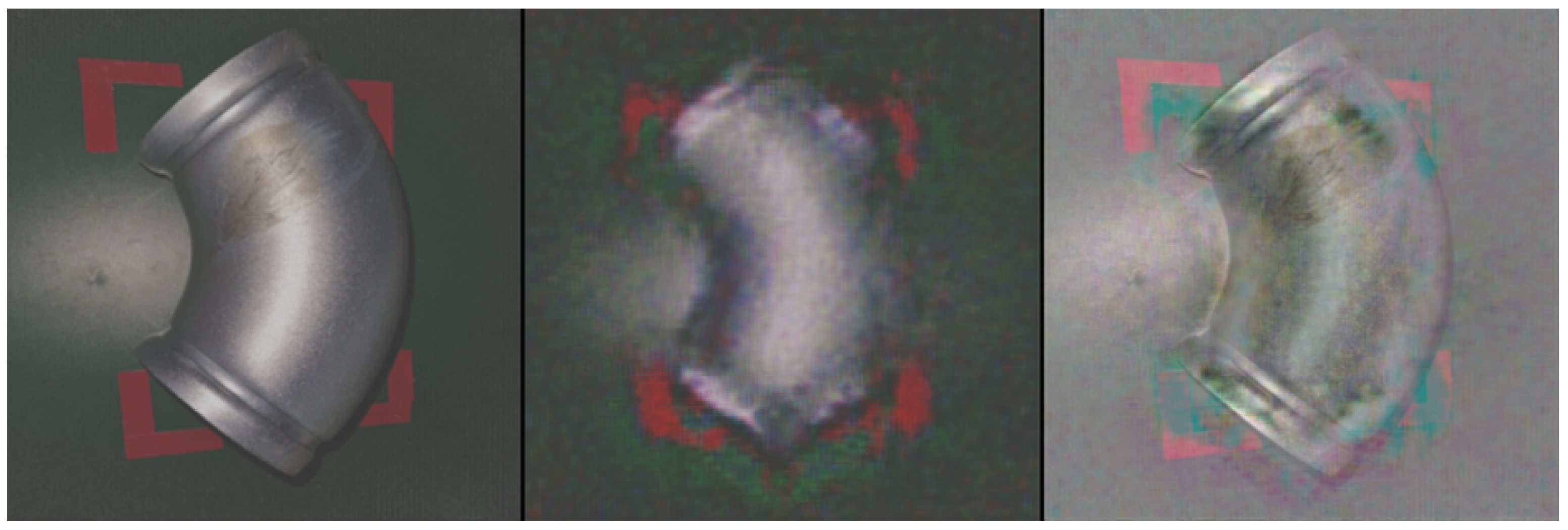
2.4. Localization & Threshold
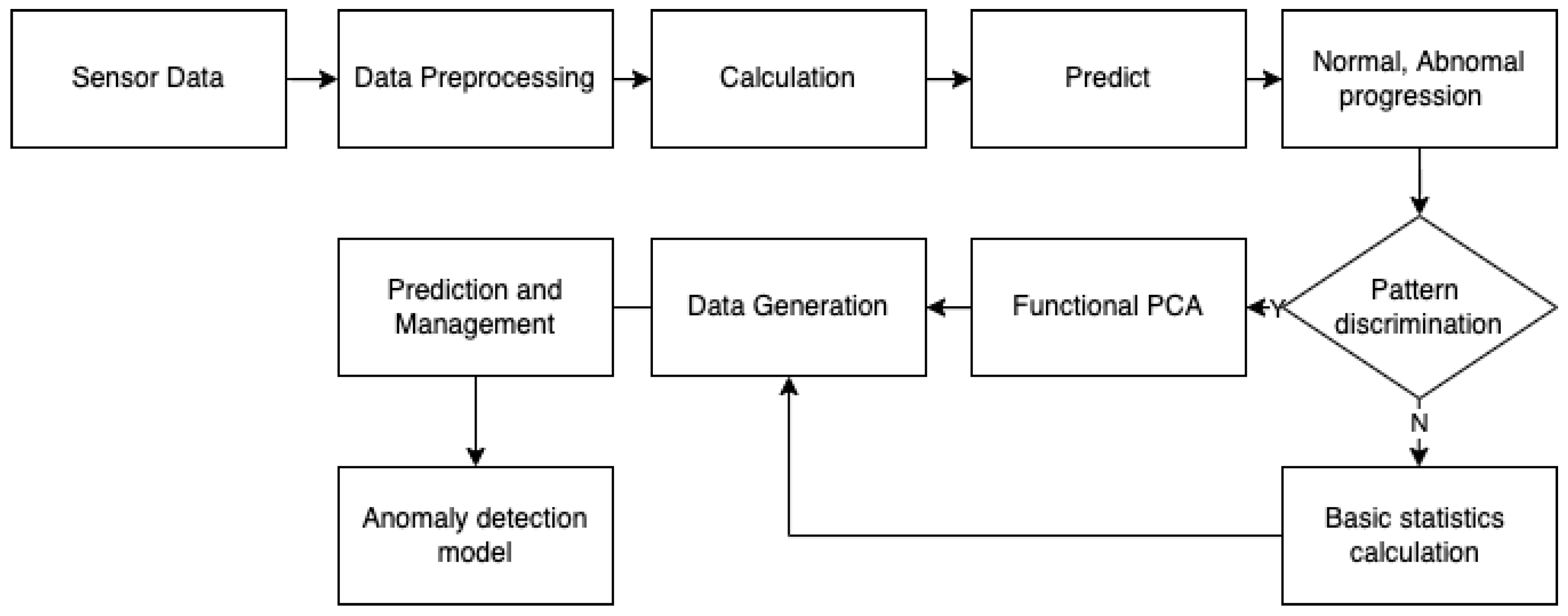
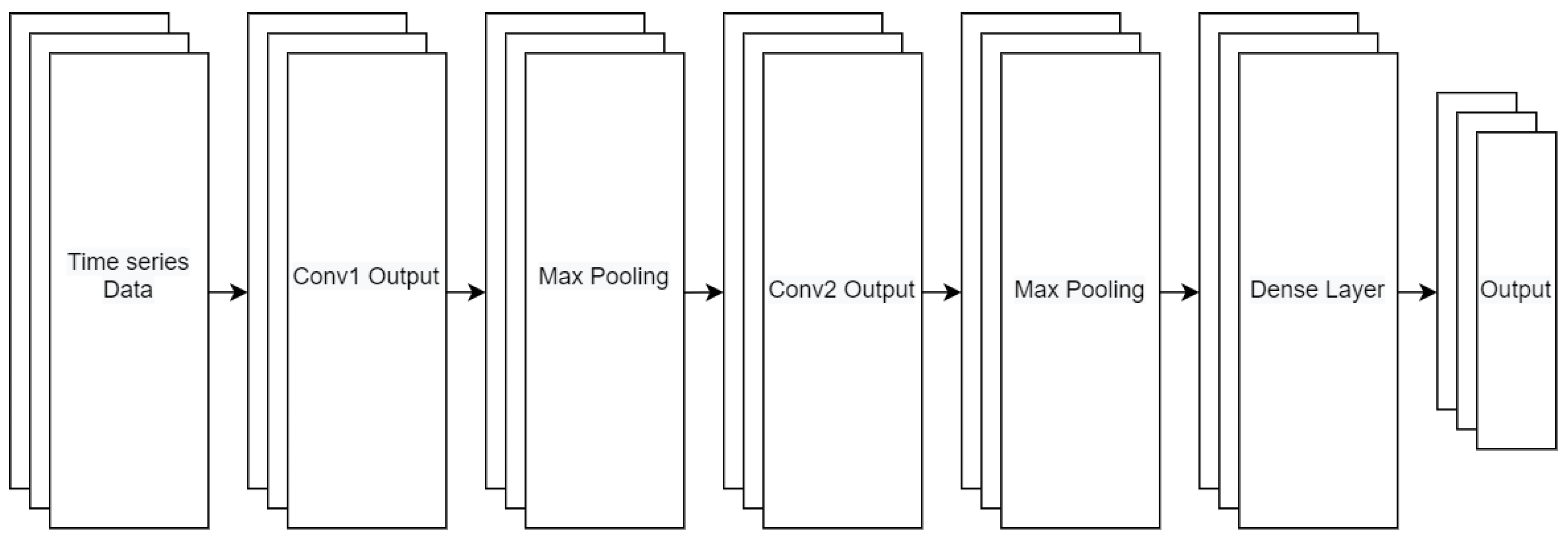
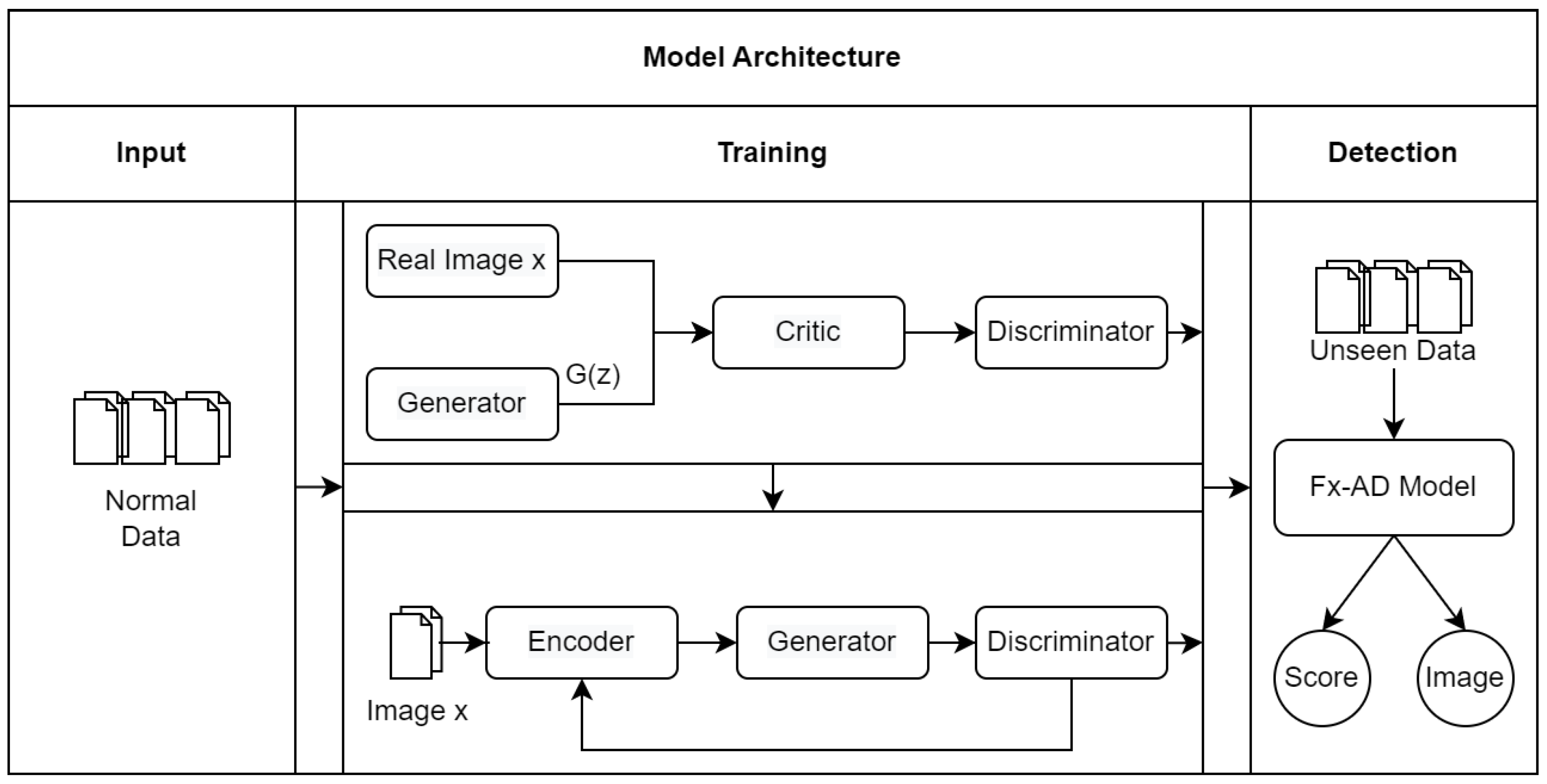
3. Fv-AD: F-AnoGAN Based Anomaly Detection
3.1. System Architecture
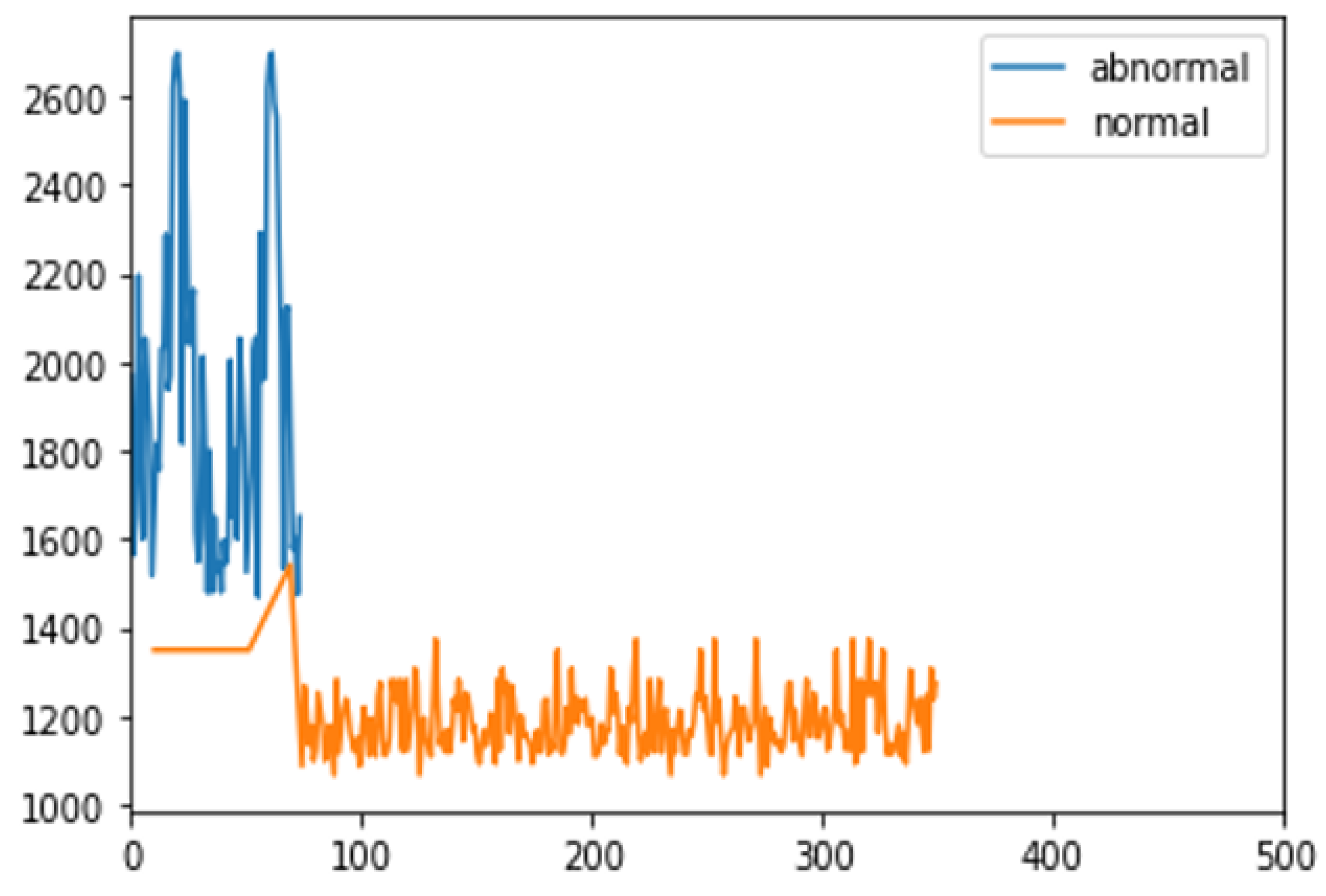
3.2. Calculating Anomaly Score
4. Experiment and Results
4.1. Experiment Environment
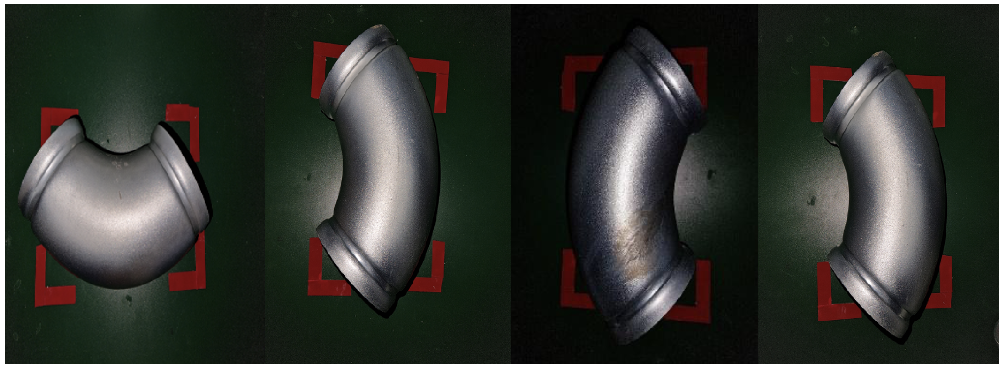
4.2. Datasets
4.3. Performance Matrix
4.4. Results and Analysis
5. Conclusions
Author Contributions
Funding
Institutional Review Board Statement
Informed Consent Statement
Data Availability Statement
Acknowledgments
Conflicts of Interest
References
- Goodfellow, I.; Pouget-Abadie, J.; Mirza, M.; Xu, B.; Warde-Farley, D.; Ozair, S.; Courville, A.; Bengio, Y. Generative adversarial nets. In Proceedings of the 28th Annual Conference on Neural Information Processing Systems (NIPS 2014), Montreal, QC, Canada, 8–13 December 2014. [Google Scholar]
- Radford, A.; Metz, L.; Chintala, S. Unsupervised representation learning with deep convolutional generative adversarial networks. arXiv 2015, arXiv:1511.06434. [Google Scholar]
- Pham, H.; Dai, Z.; Xie, Q.; Le, Q.V. Meta pseudo labels. In Proceedings of the IEEE/CVF Conference on Computer Vision and Pattern Recognition, Nashville, TN, USA, 21–25 June 2021; pp. 11557–11568. [Google Scholar]
- Chalapathy, R.; Chawla, S. Deep learning for anomaly detection: A survey. arXiv 2019, arXiv:1901.03407. [Google Scholar]
- Schlegl, T.; Seeböck, P.; Waldstein, S.M.; Langs, G.; Schmidt-Erfurth, U. f-AnoGAN: Fast unsupervised anomaly detection with generative adversarial networks. Med. Image Anal. 2019, 54, 30–44. [Google Scholar] [CrossRef] [PubMed]
- Lee, K.; Lim, J.; Bok, K.; Yoo, J. Handling method of imbalance data for machine learning: Focused on sampling. J. Korea Contents Assoc. 2019, 19, 567–577. [Google Scholar]
- Li, Z.; Kamnitsas, K.; Glocker, B. Analyzing overfitting under class imbalance in neural networks for image segmentation. IEEE Trans. Med. Imaging 2020, 40, 1065–1077. [Google Scholar] [CrossRef] [PubMed]
- Huang, Y.; Juefei-Xu, F.; Guo, Q.; Liu, Y.; Pu, G. FakeLocator: Robust localization of GAN-based face manipulations. IEEE Trans. Inf. Forensics Secur. 2022; Early Access. [Google Scholar] [CrossRef]
- Schlegl, T.; Seeböck, P.; Waldstein, S.M.; Schmidt-Erfurth, U.; Langs, G. Unsupervised anomaly detection with generative adversarial networks to guide marker discovery. In Proceedings of the International Conference on Information Processing in Medical Imaging, Boone, NC, USA, 25–30 June 2017; Springer: Berlin/Heidelberg, Germany, 2017; pp. 146–157. [Google Scholar]
- Nam, H. A case study on the application of process abnormal detection process using big data in smart factory. Korean J. Appl. Stat. 2021, 34, 99–114. [Google Scholar]
- Jiang, W.; Hong, Y.; Zhou, B.; He, X.; Cheng, C. A GAN-based anomaly detection approach for imbalanced industrial time series. IEEE Access 2019, 7, 143608–143619. [Google Scholar] [CrossRef]
- Lu, H.; Du, M.; Qian, K.; He, X.; Wang, K. GAN-based data augmentation strategy for sensor anomaly detection in industrial robots. IEEE Sens. J. 2021. [Google Scholar] [CrossRef]
- Kiran, B.R.; Thomas, D.M.; Parakkal, R. An overview of deep learning based methods for unsupervised and semi-supervised anomaly detection in videos. J. Imaging 2018, 4, 36. [Google Scholar] [CrossRef] [Green Version]
- Oz, M.A.N.; Mercimek, M.; Kaymakci, O.T. Anomaly localization in regular textures based on deep convolutional generative adversarial networks. Appl. Intell. 2022, 52, 1556–1565. [Google Scholar] [CrossRef]
- Munir, M.; Siddiqui, S.A.; Dengel, A.; Ahmed, S. DeepAnT: A deep learning approach for unsupervised anomaly detection in time series. IEEE Access 2018, 7, 1991–2005. [Google Scholar] [CrossRef]
- Li, D.; Chen, D.; Goh, J.; Ng, S.k. Anomaly detection with generative adversarial networks for multivariate time series. arXiv 2018, arXiv:1809.04758. [Google Scholar]
- Li, D.; Chen, D.; Jin, B.; Shi, L.; Goh, J.; Ng, S. Madgan: Multivariate anomaly detection for time series data with generative adversarial networks. In Proceedings of the International Conference on Artificial Neural Networks, Munich, Germany, 17–19 September 2019; pp. 703–716. [Google Scholar]
- Akcay, S.; Atapour-Abarghouei, A.; Breckon, T.P. Ganomaly: Semi-supervised anomaly detection via adversarial training. In Proceedings of the Asian Conference on Computer Vision, Perth, Australia, 2–6 December 2018; Springer: Berlin/Heidelberg, Germany, 2018; pp. 622–637. [Google Scholar]
- Bae, S.; Kim, M.; Jung, H. GAN system using noise for image generation. J. Korea Inst. Inf. Commun. Eng. 2020, 24, 700–705. [Google Scholar]
- Arjovsky, M.; Chintala, S.; Bottou, L. Wasserstein generative adversarial networks. In Proceedings of the International Conference on Machine Learning, Seoul, Korea, 15–17 November 2017; pp. 214–223. [Google Scholar]
- Gulrajani, I.; Ahmed, F.; Arjovsky, M.; Dumoulin, V.; Courville, A.C. Improved training of wasserstein gans. In Proceedings of the 31st Annual Conference on Neural Information Processing Systems (NIPS 2017), Long Beach, CA, USA, 4–9 December 2017. [Google Scholar]
- Berg, A.; Ahlberg, J.; Felsberg, M. Unsupervised learning of anomaly detection from contaminated image data using simultaneous encoder training. arXiv 2019, arXiv:1905.11034. [Google Scholar]
- Mao, X.; Li, Q.; Xie, H.; Lau, R.Y.; Wang, Z.; Paul Smolley, S. Least squares generative adversarial networks. In Proceedings of the IEEE International Conference on Computer Vision, Venice, Italy, 22–29 October 2017; pp. 2794–2802. [Google Scholar]
- Karras, T.; Aila, T.; Laine, S.; Lehtinen, J. Progressive growing of gans for improved quality, stability, and variation. arXiv 2017, arXiv:1710.10196. [Google Scholar]
- Ledig, C.; Theis, L.; Huszár, F.; Caballero, J.; Cunningham, A.; Acosta, A.; Aitken, A.; Tejani, A.; Totz, J.; Wang, Z.; et al. Photo-realistic single image super-resolution using a generative adversarial network. In Proceedings of the IEEE Conference on Computer Vision and Pattern Recognition, Honolulu, HI, USA, 21–26 July 2017; pp. 4681–4690. [Google Scholar]
- Venkataramanan, S.; Peng, K.C.; Singh, R.V.; Mahalanobis, A. Attention guided anomaly localization in images. In Proceedings of the European Conference on Computer Vision, Glasgow, UK, 23–28 August 2020; Springer: Berlin/Heidelberg, Germany, 2020; pp. 485–503. [Google Scholar]
- Park, C.H.; Kim, T.; Kim, J.; Choi, S.; Lee, G.H. Outlier Detection By Clustering-Based Ensemble Model Construction. KIPS Trans. Softw. Data Eng. 2018, 7, 435–442. [Google Scholar]
- Yoo, J.; Choo, J. A study on the test and visualization of change in structures associated with the occurrence of non-stationary of long-term time series data based on unit root test. KIPS Trans. Softw. Data Eng. 2019, 8, 289–302. [Google Scholar]
- Vincent, P.; Larochelle, H.; Bengio, Y.; Manzagol, P.A. Extracting and composing robust features with denoising autoencoders. In Proceedings of the 25th International Conference on Machine Learning, Helsinki, Finland, 5–9 July 2008; pp. 1096–1103. [Google Scholar]
- Pathak, D.; Krahenbuhl, P.; Donahue, J.; Darrell, T.; Efros, A.A. Context encoders: Feature learning by inpainting. In Proceedings of the IEEE Conference on Computer Vision and Pattern Recognition, Las Vegas, NV, USA, 27–30 June 2016; pp. 2536–2544. [Google Scholar]
- Salimans, T.; Goodfellow, I.; Zaremba, W.; Cheung, V.; Radford, A.; Chen, X. Improved techniques for training gans. In Proceedings of the 30th Annual Conference on Neural Information Processing Systems (NIPS 2016), Barcelona, Spain, 5–10 December 2016. [Google Scholar]
- Platform, K.A.M.P. (Korea AI Manufacturing Platform) CNC Machine AI Dataset, KAIST (UNIST, EPM SOLUTIONS). 2022. Available online: https://www.kamp-ai.kr/front/dataset/AiData.jsp (accessed on 11 June 2020).
- Das, A.; Rad, P. Opportunities and challenges in explainable artificial intelligence (XAI): A survey. arXiv 2020, arXiv:2006.11371. [Google Scholar]
- Bentley, K.H.; Kleiman, E.M.; Elliott, G.; Huffman, J.C.; Nock, M.K. Real-time monitoring technology in single-case experimental design research: Opportunities and challenges. Behav. Res. Ther. 2019, 117, 87–96. [Google Scholar] [CrossRef] [PubMed]


| Type | Label | Image_distance | Anomaly_score | Z_distance | Loss |
|---|---|---|---|---|---|
| Class | 1 | ||||
| 1 | |||||
| 1 | |||||
| 1 | |||||
| 1 | |||||
| … | … | … | … | … | |
| 1 | |||||
| 1 | |||||
| 1 | |||||
| 1 | |||||
| 1 | |||||
| Mean | 1 |
| Type | Label | Image_distance | Anomaly_score | Z_distance | Loss |
|---|---|---|---|---|---|
| Class | 0 | ||||
| 0 | |||||
| 0 | |||||
| 0 | |||||
| 0 | |||||
| … | … | … | … | … | |
| 0 | |||||
| 0 | |||||
| 0 | |||||
| 0 | |||||
| 0 | |||||
| Mean | 0 |
| Precision | Sensitivity | Specificity | F1-Score | AUC | |
|---|---|---|---|---|---|
| 0.923 | 0.957 | 0.966 | 0.927 | 0.942 | |
| 0.908 | 0.921 | 0.951 | 0.894 | 0.931 | |
| 0.978 | 0.981 | 0.982 | 0.971 | 0.997 |
| Precision | Sensitivity | Specificity | F1-Score | AUC | |
|---|---|---|---|---|---|
| CNN | 0.952 | 0.969 | 0.971 | 0.963 | 0.993 |
| AE | 0.964 | 0.974 | 0.981 | 0.951 | 0.978 |
| AnoGAN | 0.928 | 0.983 | 0.980 | 0.931 | 0.964 |
| Fv-AD | 0.978 | 0.981 | 0.982 | 0.971 | 0.997 |
Publisher’s Note: MDPI stays neutral with regard to jurisdictional claims in published maps and institutional affiliations. |
© 2022 by the authors. Licensee MDPI, Basel, Switzerland. This article is an open access article distributed under the terms and conditions of the Creative Commons Attribution (CC BY) license (https://creativecommons.org/licenses/by/4.0/).
Share and Cite
Park, C.; Lim, S.; Cha, D.; Jeong, J. Fv-AD: F-AnoGAN Based Anomaly Detection in Chromate Process for Smart Manufacturing. Appl. Sci. 2022, 12, 7549. https://doi.org/10.3390/app12157549
Park C, Lim S, Cha D, Jeong J. Fv-AD: F-AnoGAN Based Anomaly Detection in Chromate Process for Smart Manufacturing. Applied Sciences. 2022; 12(15):7549. https://doi.org/10.3390/app12157549
Chicago/Turabian StylePark, Chanho, Sumin Lim, Daniel Cha, and Jongpil Jeong. 2022. "Fv-AD: F-AnoGAN Based Anomaly Detection in Chromate Process for Smart Manufacturing" Applied Sciences 12, no. 15: 7549. https://doi.org/10.3390/app12157549
APA StylePark, C., Lim, S., Cha, D., & Jeong, J. (2022). Fv-AD: F-AnoGAN Based Anomaly Detection in Chromate Process for Smart Manufacturing. Applied Sciences, 12(15), 7549. https://doi.org/10.3390/app12157549