
Ensemble Voting Regression Based on Machine Learning for Predicting Medical Waste: A Case from Turkey
.jpg)


Abstract
:1. Introduction
2. Methods
2.1. Machine Learning Algorithms
2.1.1. Random Forest (RF)
2.1.2. Adaptive Boosting (AdaBoost)
| Algorithm 1 The AdaBoost algorithm [32] |
| Input: Dataset The weight of each training set sample produces establishes a weight vector The base learning algorithm is denoted as The number of learning rounds denoted as Process: % The weight distribution is initialized For % Train a base learner ht from D utilizing distribution Dt % The error of ht is measured % Revise the distribution, where Zt denotes the normalization factor that enables Dt+1 to be a distribution. end. Output: |
2.1.3. Gradient Boosting Machine (GBM)
2.2. Voting Regressor (VR)
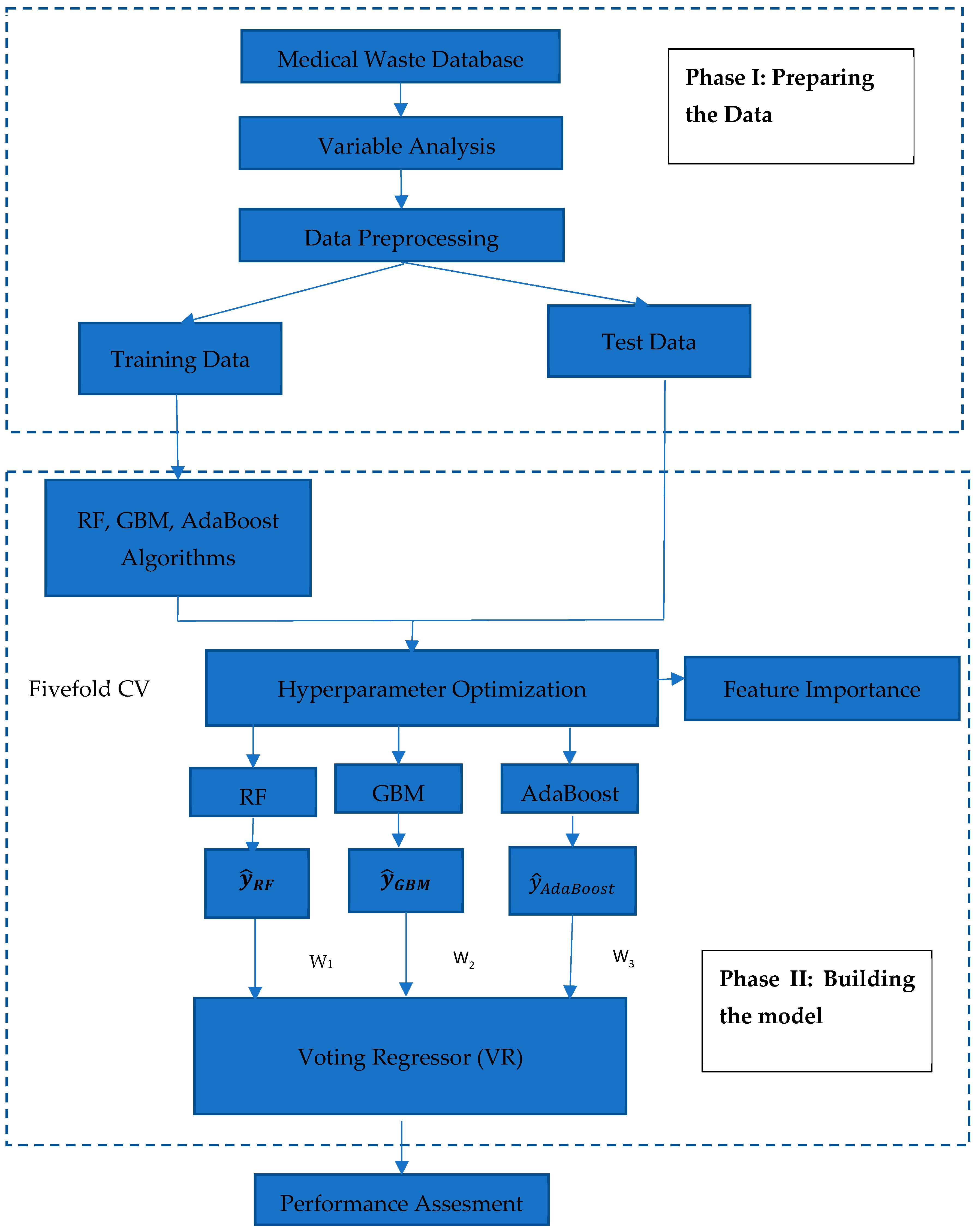
3. Proposed Model
3.1. General Context
3.2. Phase 1: Preparing the Data
3.3. Phase 2: Building the Model
- For RF, the number of trees in the forest (n_estimators) was 100, the minimum number of samples demanded to split an internal node (min_samples_split) was 2, the maximum depth of the tree (max_depth) was None, and the maximum features of each tree (max_features) was 1.
- For GBM, the shrinkage coefficient of each tree (learning_rate) was 0.1, the maximum depth of the tree (max_depth) was 3, the number of trees (n_estimators) was 100, the subsample ratio of training samples (subsample) was 1.0.
- For the AdaBoost model, the maximum number of estimators (n_estimators) was 50, learning rate (learning_rate) was 1.0.
4. Results
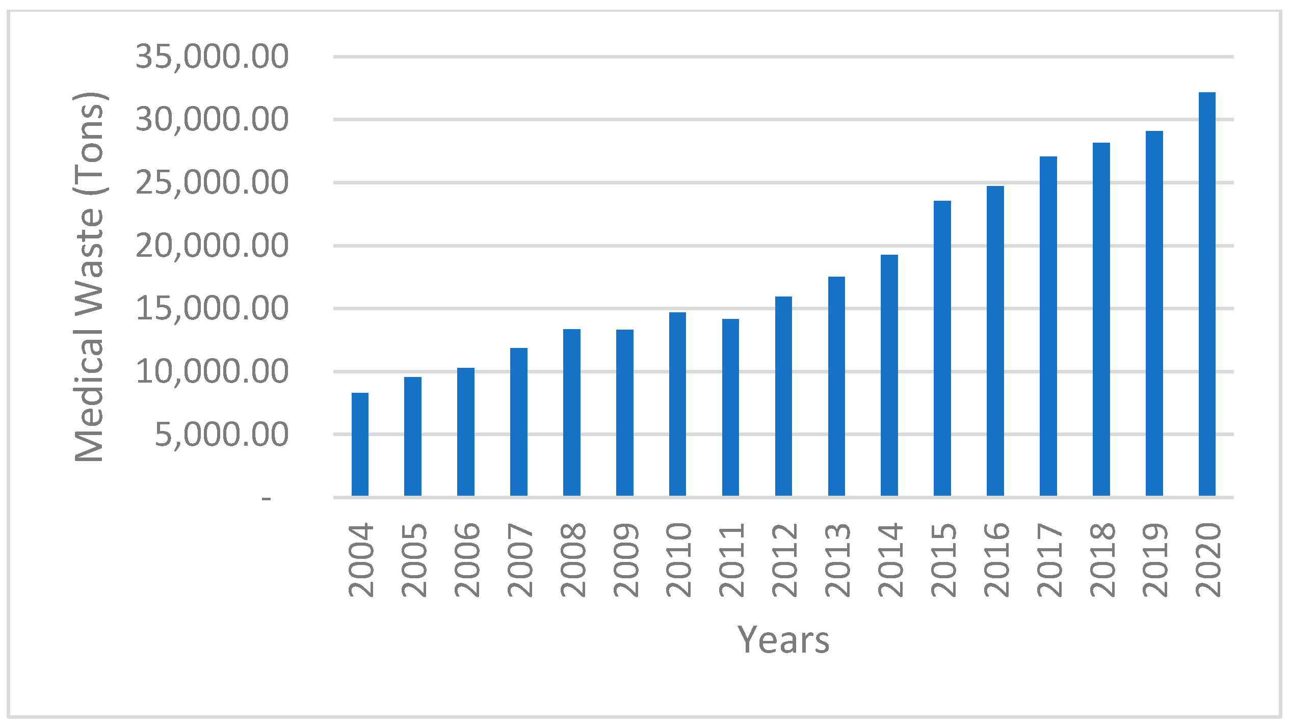
4.1. Data Acquisition
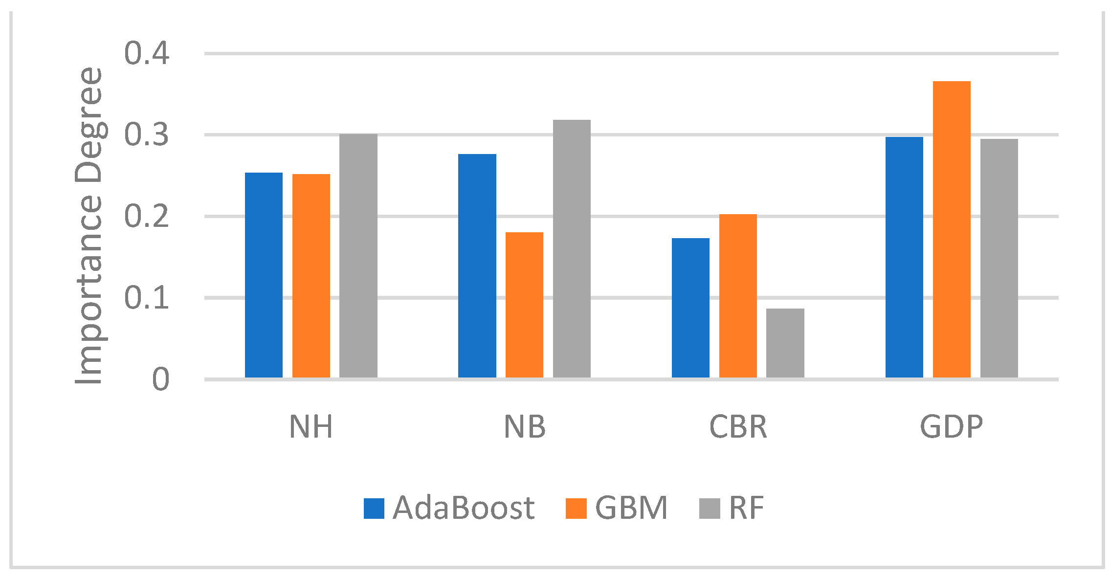
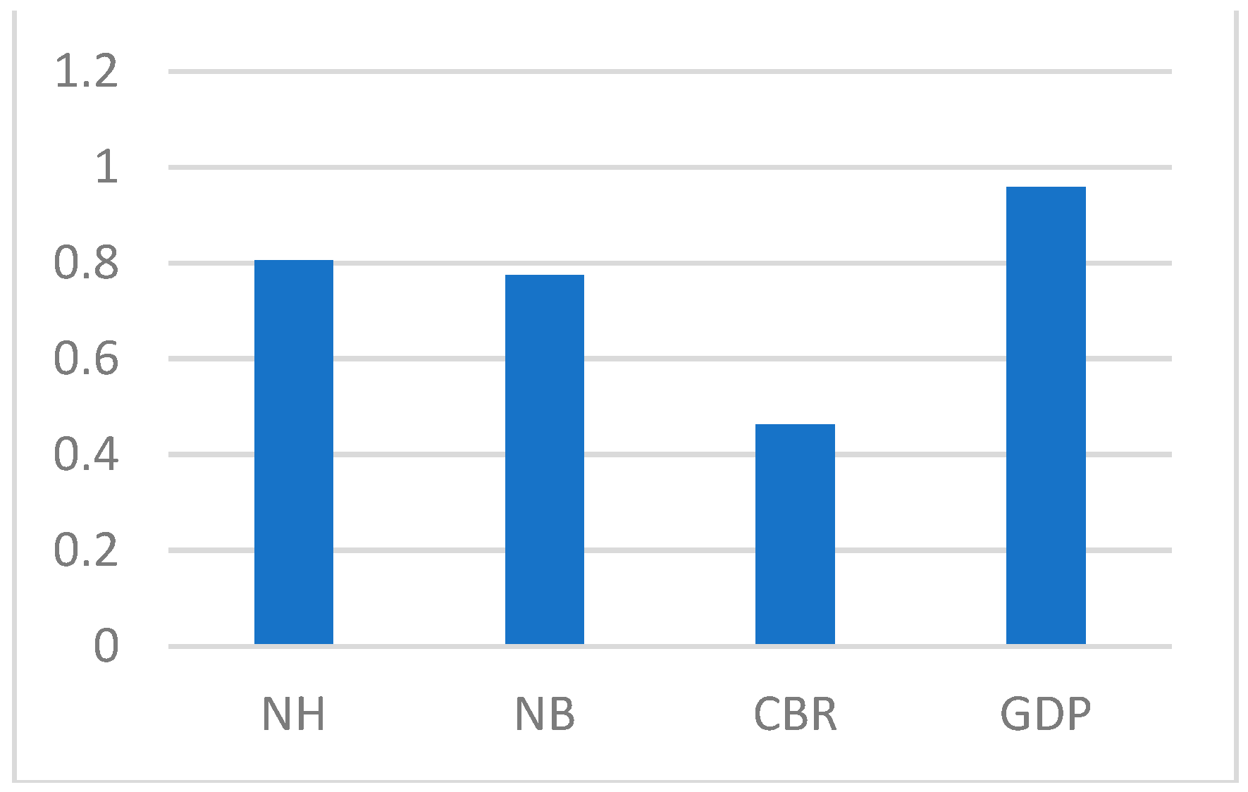
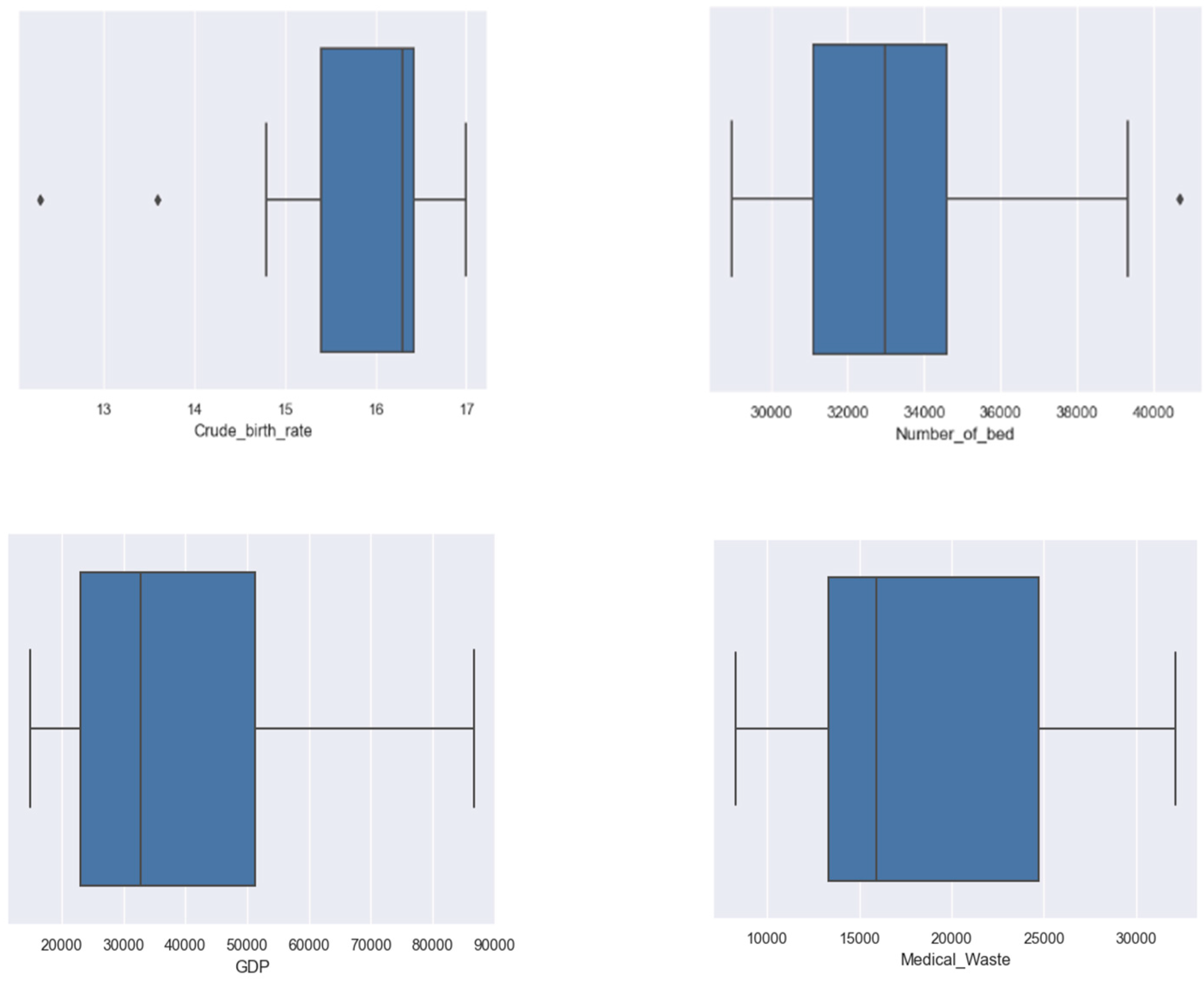
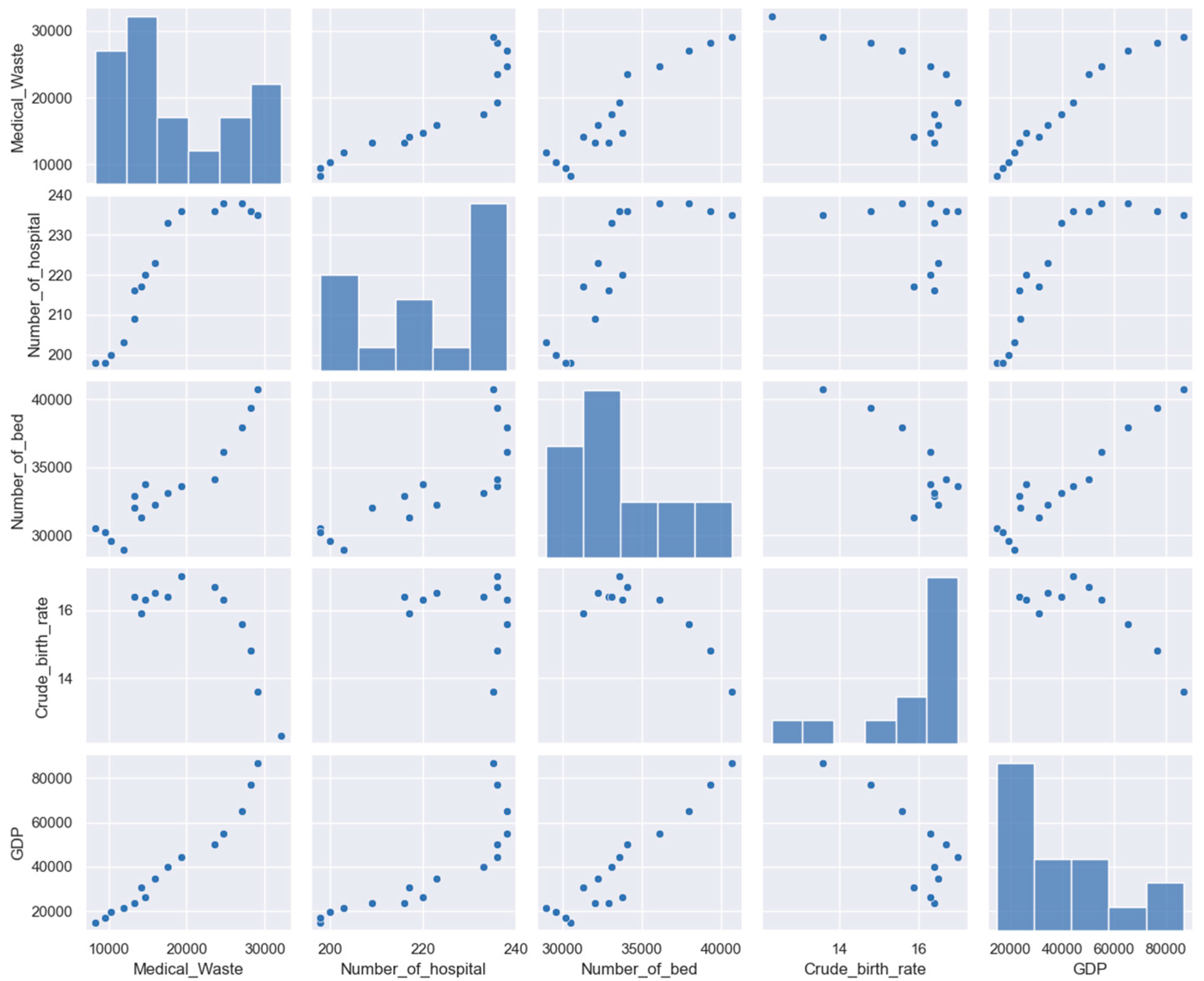
4.2. Variable Analysis
4.3. Data Preprocessing
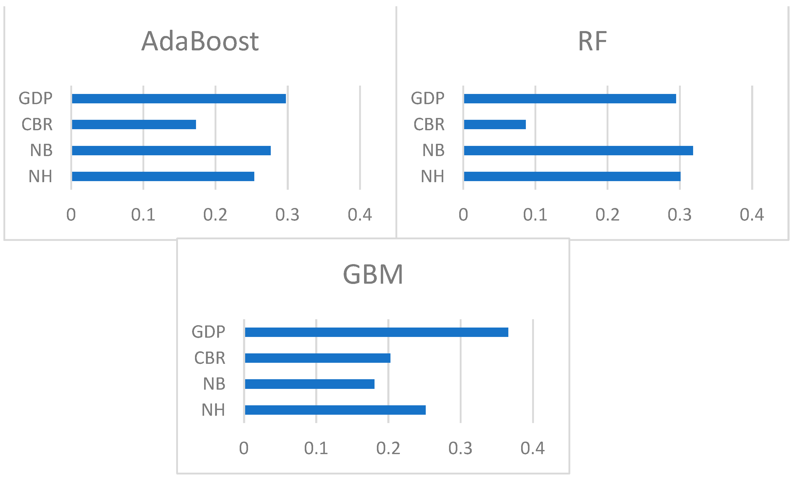
4.4. Hyperparameter Optimization
4.5. Comparison of Single ML Algorithms
4.6. Performance Assessment
5. Conclusions
Author Contributions
Funding
Institutional Review Board Statement
Informed Consent Statement
Data Availability Statement
Conflicts of Interest
References
- Ceylan, Z.; Bulkan, S.; Elevli, S. Prediction of medical waste generation using SVR, GM (1,1) and ARIMA models: A case study for megacity Istanbul. J. Environ. Health Sci. Eng. 2020, 18, 687–697. [Google Scholar] [CrossRef]
- Jahandideh, S.; Jahandideh, S.; Asadabadi, E.B.; Askarian, M.; Movahedi, M.M.; Hosseini, S.; Jahandideh, M. The use of artificial neural networks and multiple linear regression to predict rate of medical waste generation. Waste Manag. 2009, 29, 2874–2879. [Google Scholar] [CrossRef]
- Golbaz, S.; Nabizadeh, R.; Sajadi, H.S. Comparative study of predicting hospital solid waste generation using multiple linear regression and artificial intelligence. J. Environ. Health Sci. Eng. 2019, 17, 41–51. [Google Scholar] [CrossRef]
- Shinee, E.; Gombojav, E.; Nishimura, A.; Hamajima, N.; Ito, K. Healthcare waste management in the capital city of Mongolia. Waste Manag. 2008, 28, 435–441. [Google Scholar] [CrossRef]
- Nie, L.; Qiao, Z.; Wu, H. Medical Waste Management in China: A Case Study of Xinxiang. J. Environ. Prot. 2014, 5, 803–810. [Google Scholar] [CrossRef] [Green Version]
- Tirkolaee, E.B.; Abbasian, P.; Weber, G.-W. Sustainable fuzzy multi-trip location-routing problem for medical waste management during the COVID-19 outbreak. Sci. Total Environ. 2020, 756, 143607. [Google Scholar] [CrossRef]
- Uysal, F.; Tinmaz, E. Medical waste management in Trachea region of Turkey: Suggested remedial action. Waste Manag. Res. 2004, 22, 403–407. [Google Scholar] [CrossRef]
- Birpınar, M.E.; Bilgili, M.S.; Erdoğan, T. Medical waste management in Turkey: A case study of Istanbul. Waste Manag. 2009, 29, 445–448. [Google Scholar] [CrossRef]
- Nguyen, X.C.; Nguyen, T.T.H.; La, D.D.; Kumar, G.; Rene, E.R.; Nguyen, D.D.; Chang, S.W.; Chung, W.J.; Nguyen, X.H.; Nguyen, V.K. Development of Machine Learning—Based Models to Forecast Solid Waste Generation in Residential Areas: A Case Study from Vietnam. Resour. Conserv. Recycl. 2021, 167, 105381. [Google Scholar] [CrossRef]
- Tesfahun, E.; Kumie, A.; Beyene, A. Developing models for the prediction of hospital healthcare waste generation rate. Waste Manag. Res. 2015, 34, 75–80. [Google Scholar] [CrossRef]
- Çetinkaya, A.Y.; Kuzu, S.L.; Demir, A. Medical waste management in a mid-populated Turkish city and development of medical waste prediction model. Environ. Dev. Sustain. 2019, 22, 6233–6244. [Google Scholar] [CrossRef]
- Idowu, I.; Alo, B.; Atherton, W.; Al Khaddar, R. Profile of medical waste management in two healthcare facilities in Lagos, Nigeria: A case study. Waste Manag. Res. 2013, 31, 494–501. [Google Scholar] [CrossRef]
- Al-Khatib, I.A.; Fkhidah, I.A.; Khatib, J.I.; Kontogianni, S. Implementation of a multi-variable regression analysis in the assessment of the generation rate and composition of hospital solid waste for the design of a sustainable management system in developing countries. Waste Manag. Res. 2010, 34, 225–234. [Google Scholar] [CrossRef] [PubMed]
- Bdour, A.; Altrabsheh, B.; Hadadin, N.; Al-Shareif, M. Assessment of medical wastes management practice: A case study of the northern part of Jordan. Waste Manag. 2007, 27, 746–759. [Google Scholar] [CrossRef] [PubMed]
- Sabour, M.R.; Mohamedifard, A.; Kamalan, H. A mathematical model to predict the composition and generation of hospital wastes in Iran. Waste Manag. 2007, 27, 584–587. [Google Scholar] [CrossRef]
- Korkut, E.N. Estimations and analysis of medical waste amounts in the city of Istanbul and proposing a new approach for the estimation of future medical waste amounts. Waste Manag. 2018, 81, 168–176. [Google Scholar] [CrossRef]
- Chauhan, A.; Singh, A. An ARIMA model for the forecasting of healthcare waste generation in the Garhwal region of Uttarakhand, India. Int. J. Serv. Oper. Inform. 2017, 8, 352. [Google Scholar] [CrossRef]
- Karpušenkaitė, A.; Ruzgas, T.; Denafas, G. Forecasting medical waste generation using short and extra short datasets: Case study of Lithuania. Waste Manag. Res. 2016, 34, 378–387. [Google Scholar] [CrossRef]
- Karpušenkaitė, A.; Ruzgas, T.; Denafas, G. Time-series-based hybrid mathematical modelling method adapted to forecast automotive and medical waste generation: Case study of Lithuania. Waste Manag. Res. 2018, 36, 454–462. [Google Scholar] [CrossRef]
- Thakur, V.; Ramesh, A. Analyzing composition and generation rates of biomedical waste in selected hospitals of Uttarakhand, India. J. Mater. Cycles Waste Manag. 2017, 20, 877–890. [Google Scholar] [CrossRef]
- Papacharalampous, G.; Tyralis, H.; Koutsoyiannis, D. Univariate Time Series Forecasting of Temperature and Precipitation with a Focus on Machine Learning Algorithms: A Multiple-Case Study from Greece. Water Resour. Manag. 2018, 32, 5207–5239. [Google Scholar] [CrossRef]
- Pavlyshenko, B.M. Machine-Learning Models for Sales Time Series Forecasting. Data 2019, 4, 15. [Google Scholar] [CrossRef] [Green Version]
- Dissanayaka, D.; Vasanthapriyan, S. Forecast municipal solid waste generation in Sri Lanka. In Proceedings of the 2019 International Conference on Advancements in Computing, Malabe, Sri Lanka, 5–7 December 2019; pp. 210–215. [Google Scholar] [CrossRef]
- Meleko, A.; Adane, A. Assessment of Health Care Waste Generation Rate and Evaluation of its Management System in Mizan Tepi University Teaching Hospital (MTUTH), Bench Maji Zone, South West Ethiopia. Ann. Rev. Res. 2018, 1, 555566. [Google Scholar] [CrossRef]
- Kilimci, Z.H. Ensemble Regression-Based Gold Price (XAU/USD) Prediction. J. Emerg. Comput. Technol. 2022, 2, 7–12. [Google Scholar]
- Yang, N.-C.; Ismail, H. Voting-Based Ensemble Learning Algorithm for Fault Detection in Photovoltaic Systems under Different Weather Conditions. Mathematics 2022, 10, 285. [Google Scholar] [CrossRef]
- Phyo, P.-P.; Byun, Y.-C.; Park, N. Short-Term Energy Forecasting Using Machine-Learning-Based Ensemble Voting Regression. Symmetry 2022, 14, 160. [Google Scholar] [CrossRef]
- Pham, T.A.; Vu, H.-L.T. Application of Ensemble Learning Using Weight Voting Protocol in the Prediction of Pile Bearing Capacity. Math. Probl. Eng. 2021, 2021, 1–14. [Google Scholar] [CrossRef]
- Bhuiyan, A.M.; Sahi, R.K.; Islam, R.; Mahmud, S. Machine Learning Techniques Applied to Predict Tropospheric Ozone in a Semi-Arid Climate Region. Mathematics 2021, 9, 2901. [Google Scholar] [CrossRef]
- Bayahya, A.Y.; Alhalabi, W.; Alamri, S.H. Older Adults Get Lost in Virtual Reality: Visuospatial Disorder Detection in Dementia Using a Voting Approach Based on Machine Learning Algorithms. Mathematics 2022, 10, 1953. [Google Scholar] [CrossRef]
- Liang, W.; Luo, S.; Zhao, G.; Wu, H. Predicting Hard Rock Pillar Stability Using GBDT, XGBoost, and LightGBM Algorithms. Mathematics 2020, 8, 765. [Google Scholar] [CrossRef]
- Li, Y.; Chen, W. A Comparative Performance Assessment of Ensemble Learning for Credit Scoring. Mathematics 2020, 8, 1756. [Google Scholar] [CrossRef]
- Gutierrez, G. Artificial Intelligence in the Intensive Care Unit. Crit. Care 2020, 24, 101. [Google Scholar] [CrossRef] [Green Version]
- Breiman, L. Bagging predictors. Mach. Learn. 1996, 24, 123–140. [Google Scholar] [CrossRef] [Green Version]
- Byeon, H. Exploring Factors for Predicting Anxiety Disorders of the Elderly Living Alone in South Korea Using Interpretable Machine Learning: A Population-Based Study. Int. J. Environ. Res. Public Health 2021, 18, 7625. [Google Scholar] [CrossRef]
- Ahmad, M.; Kamiński, P.; Olczak, P.; Alam, M.; Iqbal, M.; Ahmad, F.; Sasui, S.; Khan, B. Development of Prediction Models for Shear Strength of Rockfill Material Using Machine Learning Techniques. Appl. Sci. 2021, 11, 6167. [Google Scholar] [CrossRef]
- Freund, Y.; Schapire, R.E. Experiments with a New Boosting Algorithm. In Proceedings of the 13th International Conference on Machine Learning, Bari, Italy, 3–6 July 1996; pp. 148–156. [Google Scholar]
- Friedman, J.H. Greedy function approximation: A gradient boosting machine. Ann. Stat. 2001, 29, 1189–1232. [Google Scholar] [CrossRef]
- How to Develop a Weighted Average Ensemble With Python. Available online: https://machinelearningmastery.com/weighted-average-ensemble-with-python/#:~:text=Weighted%20average%20or%20weighted%20sum%20ensemble%20is%20an%20ensemble%20machine,related%20to%20the%20voting%20ensemble (accessed on 14 May 2022).
- İstanbul Metropolitan Municipality Department Open Data Portal. Available online: https://data.ibb.gov.tr/en/dataset/tibbi-atik-miktari/resource/474d4b1c-6cd4-4626-8a69-d9c269d3809 (accessed on 6 June 2021).
- The Official Website of Turkish Statistics Institute. Available online: https://biruni.tuik.gov.tr/medas/ (accessed on 10 June 2021).
- Schwertman, N.C.; Owens, M.A.; Adnan, R. A simple more general boxplot method for identifying outliers. Comput. Stat. Data Anal. 2004, 47, 165–174. [Google Scholar] [CrossRef]
- Ramírez-Gallego, S.; Krawczyk, B.; García, S.; Woźniak, M.; Herrera, F. A survey on data preprocessing for data stream mining: Current status and future directions. Neurocomputing 2017, 239, 39–57. [Google Scholar] [CrossRef]
- Kwak, S.K.; Kim, J.H. Statistical data preparation: Management of missing values and outliers. Korean J. Anesthesiol. 2017, 70, 407–411. [Google Scholar] [CrossRef]
- Scikit-Learn. Available online: https://scikit-learn.org/ (accessed on 3 June 2022).
- A Practical Introduction to Grid Search, Random Search, and Bayes Search. Available online: https://towardsdatascience.com/a-practical-introduction-to-grid-search-random-search-and-bayes-search-d5580b1d941d (accessed on 3 June 2022).
- Awad, A.R.; Obeidat, M.; Al-Shareef, M. Mathematical-Statistical Models of Generated Hazardous Hospital Solid Waste. Int. J. Environ. Waste Manag. 2004, 39, 315–327. [Google Scholar] [CrossRef]
- Daskalopoulos, E.; Badr, O.; Probert, S. Municipal solid waste: A prediction methodology for the generation rate and composition in the European Union countries and the United States of America. Resour. Conserv. Recycl. 1998, 24, 155–166. [Google Scholar] [CrossRef]


| Reference | Data Source | Methods | Performance Measures |
|---|---|---|---|
| [1] | Official data | LR, SVR, GM (1,1), and ARIMA | R-squared, RMSE, MAD, MAPE |
| [2] | Surveys | MLR, ANN | MAE, RMSE, R-squared |
| [3] | Survey | MLR and neuron- and kernel-based methods | R-squared, MSE |
| [10] | Survey | MLR | R-squared |
| [11] | Survey | MLR | MBE, MAPE |
| [12] | Survey | MLR | R-squared |
| [13] | Survey | MLR | R-squared |
| [14] | Survey | MLR | R-squared |
| [15] | Survey | MLR | R-squared |
| [16] | Official data | LR | R-squared |
| [17] | Official data | ARIMA | MAPE, MAE |
| [18] | Official data | ANN, MLR, PLS, and SVM | R-squared, RMSE, MAE, MAPE |
| [19] | Official data | MA, Holt’s | MAPE |
| [20] | Survey | MLR, ANN | MAE, RMSE, R-squared |
| Category | Description | Mean | Standard Deviation | Min | Max |
|---|---|---|---|---|---|
| MW | Amount of the medical waste per year | 18,407.8 | 7579.8 | 8279.3 | 32,143.8 |
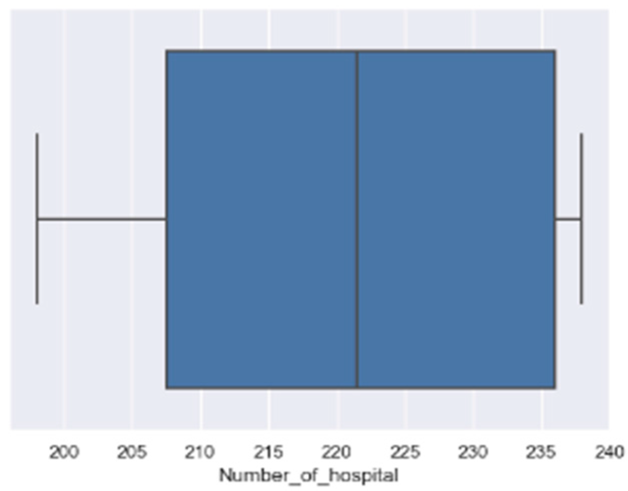
| NH | Total hospital per year | 221 | 15.5 | 198 | 238 |
| NB | Total beds per year | 33,522.3 | 3441.2 | 28,958 | 40,697 |
| CBR | The ratio of the number of live births during a year to the average population in that year, expressed per 1000 persons | 15.7 | 1.4 | 12.3 | 17 |
| GDP | Total monetary value of all final goods and services produced (and sold on the market) within a country during a year. | 39,334.1 | 22,085.7 | 14,795 | 86,798 |
| Algorithm | Hyperparameters | Meanings | Search Values | Optimal Values |
|---|---|---|---|---|
| RF | max_depth max_features n_estimators min_samples_split | Maximum depth of tree Maximum features of each tree Number of trees Minimum number of samples for leaf nodes | (5, 8, None) (3, 5, 15) (200, 500) (2, 5, 8) | 5 3 500 2 |
| GBM | learning_rate max_depth n_estimators subsample | Shrinkage coefficient of each tree Maximum depth of tree Number of trees Subsample ratio of training samples | (0.01, 0.1) (3, 8) (500, 1000) (1, 0.5, 0.7) | 0.1 8 1000 0.5 |
| AdaBoost | learning_rate n|estimators | Shrinkage coefficient of each tree Number of trees | (0.01, 0.1) (500, 1000) | 0.01 1000 |
| Models | MAE | RMSE | R-Squared | MAPE |
|---|---|---|---|---|
| RF | 1093.342 | 868.734 | 0.959 | 0.050 |
| GBM | 1332.665 | 1117.195 | 0.939 | 0.064 |
| AdaBoost | 3349.578 | 2698.408 | 0.615 | 0.153 |
| MAE | RMSE | R-Squared | MAPE | |
|---|---|---|---|---|
| Ensemble VR | 843.702 | 922.042 | 0.970 | 0.057 |
Publisher’s Note: MDPI stays neutral with regard to jurisdictional claims in published maps and institutional affiliations. |
© 2022 by the authors. Licensee MDPI, Basel, Switzerland. This article is an open access article distributed under the terms and conditions of the Creative Commons Attribution (CC BY) license (https://creativecommons.org/licenses/by/4.0/).
Share and Cite
Erdebilli, B.; Devrim-İçtenbaş, B. Ensemble Voting Regression Based on Machine Learning for Predicting Medical Waste: A Case from Turkey. Mathematics 2022, 10, 2466. https://doi.org/10.3390/math10142466
Erdebilli B, Devrim-İçtenbaş B. Ensemble Voting Regression Based on Machine Learning for Predicting Medical Waste: A Case from Turkey. Mathematics. 2022; 10(14):2466. https://doi.org/10.3390/math10142466
Chicago/Turabian StyleErdebilli, Babek, and Burcu Devrim-İçtenbaş. 2022. "Ensemble Voting Regression Based on Machine Learning for Predicting Medical Waste: A Case from Turkey" Mathematics 10, no. 14: 2466. https://doi.org/10.3390/math10142466
APA StyleErdebilli, B., & Devrim-İçtenbaş, B. (2022). Ensemble Voting Regression Based on Machine Learning for Predicting Medical Waste: A Case from Turkey. Mathematics, 10(14), 2466. https://doi.org/10.3390/math10142466