Abstract
The analysis of air pollution behavior is becoming crucial, where information on air pollution behavior is vital for managing air quality events. Many studies have described the stochastic behavior of air pollution based on the Markov chain (MC) models. Fitting the optimum order of MC models is essential for describing the stochastic process. However, uncertainty remains concerning the optimum order of such models for representing and characterizing air pollution index (API) data. In this study, the optimum order of the MC models for hourly and daily API sequences from seven stations in the central region of Peninsular Malaysia is identified, based on the Bayesian information criteria (BIC), contributing to exploring an adequate explanation of the probabilistic dependence of air pollution. A summary of the statistics for the API was calculated prior to the analysis. The Markov property and the divergence for the empirically estimated transition matrix of an MC sequence are also investigated. It is found from the analysis that the optimum order varies from one station to another. At most stations, for both observed and simulated API data, the second and third orders of the MC models are found to be optimum for hourly API occurrences, while the first-order MC is found to be most fitting for describing the dynamics of the daily API. Overall, fitting the optimum order of the MC model for the API data sequence captured the delay effect of air pollution. Accordingly, we concluded that the air quality standard lies within controllable limits, except for some infrequent occurrences of API values exceeding the unhealthy level.
Keywords:
chi-squared test; high-order Markov chain; log-likelihood function; Markov property; maximum likelihood estimation; R software MSC:
60J10
1. Introduction
Clean air is necessary for healthy living; however, much of the air in the atmosphere is polluted. Air pollution is an environmental phenomenon that occurs as a result of natural disasters and anthropogenic activities [1]. It is one of the most serious environmental issues that have negative impacts on people’s health and quality of life [2]. The Department of Environment (DOE) defines the air pollution index (API) as a generalized metric for characterizing the status of the air quality in the environment. The API is computed using the average indices for five major pollution variables: ozone (O3), nitric oxide (NO2), particulate matter (PM10), carbon monoxide (CO), and sulphur dioxide (SO2), and the highest value from these five subindices at a particular hour is chosen as the API value [3,4].
There are many applications of the MC model in various areas of research, where it is considered a useful tool to describe probabilistic dependence in a model for a stochastic process. MC models are widely used in many different disciplines such as in economics, environment, education, medical, business engineering, queuing networks, and manufacturing systems [5]. For example, Zhou et al. [6] have used the MC model for predicting the transition probabilities of bike rental and returns for a bike-sharing system in China. Choji et al. [7] have employed the MC model for predicting the long run of share prices for two banks in Nigeria. Saad et al. [8] have investigated the track movements of lecturers in universities using the MC model. In [9], a discrete-time MC model has been applied for analyzing job transitions in Mexico.
Among the statistical models that are widely used in environmental research, the MC model is considered a powerful model, particularly for describing the probabilistic behavior in environmental problems, as reported in the studies by [10,11,12,13]. They found that the MC is a superior model in characterizing the probabilistic behavior of environmental problems. Particularly, MC models have been used for modeling the air quality conditions in the environment and implemented to represent air pollution occurrences. For example, Larsen et al. [14] modeled air quality using ozone data for a given level of threshold based on the MC. They worked with the high-order chains that can be estimated by examining correlation plots, and transition probabilities have been estimated using the maximum likelihood method. Hoyos et al. [15] employed the MC model for modeling O3 and SO2 for evaluating the effect of air pollution events in Mexico City. Rodrigues and Achcar [16] have proposed a discrete-time MC model for ozone air pollution based on the maximum daily observations. They investigated the case of air pollution problems with maximum daily measurements and found that ozone behavior did not indicate a time-homogeneous property. Asadollahfardi et al. [17] have predicted the air pollution of PM2.5 index using a combination method of MC and artificial neural network methods.
Recently, Nebenzal and Fishbain [18] predicted the long run of air pollution using discrete-time MC models, which have precisely explained the distribution of the nitrogen levels. Mohamad et al. [19] have used the first-order MC to model the daily PM10 concentrations in Malaysia. Alyousifi et al. [20] have proposed the use of the discrete-time MC model for describing the probabilistic behavior of air pollution in Klang, Malaysia, based on API data. Alyousifi et al. [21] have improved the estimation of the transition probability matrix of the MC model, based on the Bayesian-based method under three different priors. Chen and Wu [22] have applied the MC model for online air quality monitoring data for predicting the air quality and determining the main air pollutants for a certain area in Taiwan. Alyousifi et al. [23] have introduced the spatial MC model for exploring the potential regional impact of air pollution in Malaysia. Gao [20] has implemented the discrete-time MC model for identifying the stochastic behavior of Air Quality Index data in China.
The uncertainty of the optimum order of the MC model may lead to a lack of sureness about the prediction of the future state, such as the air pollution state, and whether it depends only on the previous state, some or all past states. Uncertainty may range from falling short of certainty to an almost complete lack of conviction or knowledge, especially about an outcome or result.
Based on the reviewed studies mentioned above, as well as to the best of our knowledge, fitting the optimum order of the MC model for the API has not yet been conducted. Thus, this study aims to fit the optimum order of the MC for modeling the stochastic dependence of the API. This study considers an extension of the analysis of the stochastic dependence of the API conducted by [20,21,23], contributing to an adequate description of the probabilistic behaviors of the API in Malaysia, and estimating the transition probabilities from one state of air pollution to another. Based on a chi-squared test, the Markov property test to analyze the serial dependence or independence in the time series through testing and a divergence test for the estimated transition matrices have been investigated. The high-order MC model has been fitted to the API data in order to determine the optimum order of the MC model for describing API data. This might suggest that the future transition of the state of air pollution relies on the current k-state and is unaffected by the past states of the process, which contribute to providing an appropriate illustration of air pollution transitions that would improve the prediction of air quality status. The rest of this paper is organized as follows. Section 2 includes the research framework and the approach used for the analysis. In Section 3, a description of the dataset as well as the results and discussion are presented. Finally, the conclusions of the paper are presented in Section 4.
2. Methodology
In this section, the concepts and the main definitions of the high-order MC and the maximum likelihood estimation (MLE) of the transition probability matrix of the model are introduced. In addition, the statistical criteria for testing the Markovian property and the goodness of fit for the MC models are presented.
2.1. Discrete-Time Markov Chain Model
A stochastic process with the state space that satisfies the Markov property is called a discrete-time Markov chain (DTMC), meaning that the Markov process at time depends only on its present value at time t or , regardless of how is obtained. For every t and all states in S, we have
Suppose that Pr is the transition probability from state i to state j at time t and t + 1, respectively, which can be represented by the components of the transition probability matrix given by where for all for all and k is the number of states [24]. Each row of is a multinomial distribution. If the transition probabilities between the individual state pairs do not depend on time, the DTMC is called time-homogeneous, which is given by
where is the one-step transition probability from state i to state j in the sequence of discrete-time states, indicating that the Markov process has satisfied the Markov property. The values of ’s are the probabilities that describe the cells in the transition probability matrix of MC [25,26,27]. The quantities must satisfy the conditions , and for all i, j, . The above requirements exist because, given that we are in state i, the next state must be one of the possible states. Therefore, the sum of the rows of any state transition matrix must equal one. The MC is usually revealed by a state transition diagram in which the arrows from each state to other states illustrate transition probabilities . If there is no arrow from state i to state j, then it indicates that [26,28].
Although the first-order MC is found to be a powerful model in representing the stochastic behavior of air pollution, it cannot be assumed that the order of the model is always one because sometimes the first-order model is inadequate for explaining the data [25,29]. Thus, it could be beneficial to examine the suitability of the MC model with a higher order of dependency on its past data. In this study, a th-order MC model for or more was fitted to the API data. If the th-order MC model is fitted well to the data, this indicates that the upcoming air pollution state is affected by all the previous states when the last states of the sequence are identified. If this result is found, then the MC of order is the optimum order of the model for describing the API data. The high-order MC model may be carried out for describing the sequence of the API to be compared with the first-order MC. The th order of the MC model can be written as follows:
First-order:
Second-order:
Similarly, for the MC model of the th order, the general transition probabilities can be given as
where ; is the state space [30]. In other words, the current state of the process depends on past states, such that
In the case of , it is the first-order MC. The joint probability distribution of , which denotes the variables that represent the air pollution events in terms of the hourly API are given by , as we denote by . Then,
The transition probabilities of the MC model can be estimated based on the maximum likelihood estimate (MLE) for , which is given by
where represents the number of transitions in states i and j at time and t, respectively, and denotes the total number of transitions from i. For more details, see [31]. For estimating the parameters of the high-order MC model, the maximum likelihood function of the th order MC can be given by
where is the estimated transition probabilities of the random process that goes from state to , where is the state of the most recent observation. The superscript denotes the associated transition counts. The MLE estimators of the transition probabilities of Equation (5) can be given by
For further detail see [32,33,34].
2.2. Testing the Markov Property and Divergence for Empirically Estimated Transition Matrix of MC Sequence
In this subsection, the Markov property can be tested by using the chi-square test [31,35,36]. The test is used to assess the Markovian property, which verifies whether a given MC holds the Markov property, whereby the transition probability of the next state is dependent only on the current state. Let be a set of observations where and is the number of transitions from state i to state j and then to state m, written as , , . If the Markov property is verified, follows a Binomial distribution with the parameters and . Let
Specifically, Equation (11) involves testing the null hypothesis H0 = (verify the Markov property, ) for j, against the alternative hypothesis H1 = (does not verify the Markov property). Then the test statistic is
where S is the state space [37]. Thus, if the H0 is true, has a chi-square distribution with degrees of freedom. In addition, as applied by [38], the chi-square test can be utilized to test the divergence for an empirically estimated transition matrix of the MC sequence. Suppose is the raw count matrix and its test statistics follows a chi-square law. Then the divergence test can be written as
Concerning the Markovian property, fitting the optimum order of the MC model of the API will be determined and discussed in the following section.
2.3. Fitting the Optimum Order of the MC Model
If the Markovian property of the sequence is determined, it is then important to investigate which order fits best to the sequence under study. For fitting the most appropriate order of the MC model, the most commonly used measurements of goodness-of-fit are computed, which are the Bayesian information criterion (BIC) and Akaike’s information criterion (AIC). The statistical criterion that is widely used for selecting the appropriate orders of MC models is the Bayesian information criterion (BIC), due to its advantages in identifying the appropriate order of the MC model [38,39]. Here, BIC measures the information lost once a given model is employed to describe the API data. Hence, the BIC’s least-loss function is considered in this study for selecting the optimum order of the MC model for the hourly and daily API data. This is because AIC tends to overestimate the optimum order and may produce inconsistent results compared to the BIC [33,40,41]. Moreover, utilizing the BIC gives a mathematical formulation with a principle of parsimony in model building [42]. Therefore, according to the smallest BIC value, the optimum order of the MC model that best describes the sequence of the hourly and daily API will be determined.
The log-likelihood functions for transition probabilities are used in this criterion. The log-likelihoods for s-state MCs of order are [43]:
The formula for BIC is given by
where is the likelihood function, is the sample size, and is the number of parameters in the MC model.
3. Results and Discussion
This section presents a description of the air pollution data and the study area considered in this study. In addition, the trend analysis for air pollution, which includes the time series plots and the descriptive statistics of the air pollution data are depicted. In addition, the results of the MC modeling and the investigation of the optimum order of MC models are introduced.
3.1. Application to Air Pollution Data
The hourly and daily API data collected from seven air-monitoring stations located in the central region of Peninsular Malaysia for three years (1 January 2012–31 December 2014) were considered in modeling the transition behavior of air pollution states in this study.
Particularly, the studied stations are located in seven major cities, namely, Kuala Lumpur, Cheras, Klang, Petaling Jaya, Shah Alam, Banting, and Kuala Selangor. Figure 1 exhibits the sites of these stations in the Peninsula. For modeling the dynamics of air pollution using a discrete-time MC model, the air pollution data was divided into three categories, namely, (), (), and () that are denoted by numbers from 1 to 3, representing the moderate, unhealthy, and very unhealthy states of air pollution, respectively [18].

Figure 1.
Sites of the studied stations in Peninsular Malaysia.
3.2. Trend Analysis for the API Data
When the API value exceeds 100, the air pollution states become unhealthy, suggesting that the air quality status is harmful to public health. Thus, assessing the risk of an API that is greater than 100 is critical, particularly in urban settings. Before going into the study in-depth, some descriptive statistics and time series plots of the API time series are determined, to provide basic information about the variables in a dataset and to derive insights into the air pollution data used in this study, which might support the results of the analysis. Table 1 presents a descriptive statistics summary of the hourly API data; it is observed that the maximum API values in the year 2013 were 495 and 323 for Klang and Banting, respectively. The API’s mean, for all the stations considered, ranged from 40 to 57, indicating that the hourly API’s mean is at a moderate level for all stations. In addition, the standard deviation of the API ranged from 16 to 25, and proportions of the API values exceed 𝑢, where 𝑢 = 100, 200, and 300, indicating that some unhealthy air pollution episodes occurred in the studied area, varying from station to station.

Table 1.
Descriptive statistics of hourly air pollution index (API) in the study areas, 2012–2014.
Figure 2 illustrates the time series plots of the observed API values. The study areas of Petaling Jaya, Banting, Shah Alam, and particularly, Klang showed a more volatile fluctuation of API values because these areas hosted more observations beyond the threshold limit of 200, whereas for the areas of Cheras, Kuala Lumpur, and Kuala Selangor, the observations are found to fluctuate around a constant mean and almost all API values are below the threshold limit of 200. Most of these figures indicate that the air pollution condition in the studied areas is not severe; nonetheless, some areas require more attention than others. Furthermore, the time series plots in Figure 2 show that the areas of Klang, Shah Alam, and Banting had experienced a severe episode of haze, with serious air pollution levels among the other cities. Because of transboundary pollution, the Klang region had the worst experiences of all.
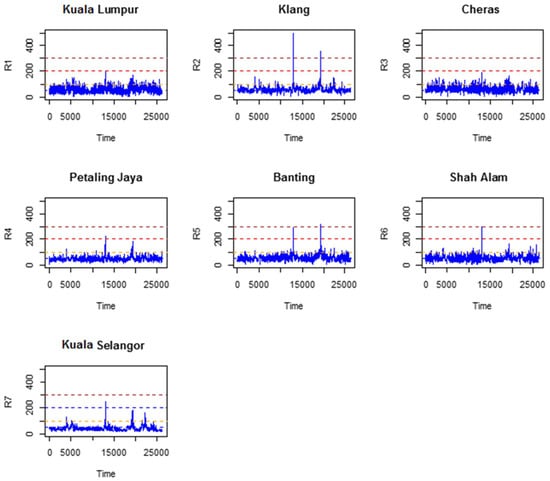
Figure 2.
Temporal trend of hourly APIs for the stations considered in this study.
3.3. The Performance of the Markov Chain Modeling
With reference to the studies by [20,21,23], air pollution behavior may be depicted as a stochastic process , where is the API value of the air pollution state at time . The random variable has values in the state space S, where , equivalent to , representing all three states. Particularly, if the process is in state 2 at time , then = 2 (or ); if it is in state 3 at time , then = 3 (or ), which can be represented by Equation (18),
Based on the studies by [20,21,23], for API data, the first-order MC can derive appropriate insights into the transition probability for the behavior of air pollution, and offers a description of the transition probability’s dependency structure in terms of time. However, it is important to examine the appropriateness of the MC with a higher order of dependency on its past data. Accordingly, in addition to the first-order MC, it might be useful to fit the high-order MC to investigate the dependency of the preceding states on the current state. This may reveal information about the dependence structures among the -lag times congruous to the hourly API transition frequency. Thus, for a preliminary examination, the autocorrelation function (ACF) of the d-time lag effect is applied, which is given by
A -order of the MC indicates that the API state is independent of its previous states when the present -lag states of the chain are identified [44,45]. Figure 3 demonstrates the ACF plot for the API sequence for each station. It is obvious that when the -time lag increases, the ACF values decrease. Hence, it will be useful to fit the high-order MC model to describe the transition behavior of the APIs. Furthermore, to introduce an accurate analysis regarding the MC model for air pollution, the first-order MC model would be compared with the high-order MC model.
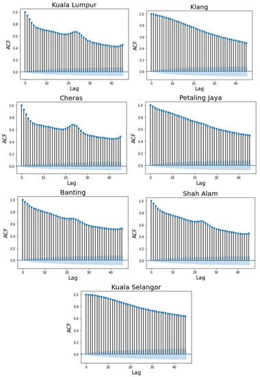
Figure 3.
Visualization of the autocorrelation function (ACF) for API data.
Although the first order of the MC model was a flexible model in describing the stochastic behavior of air pollution, as reported in the studies by [20,21,23], it cannot be assumed that the order is always one because sometimes it is inadequate to give an appropriate model [46]. In addition, the influence of being exposed to the API is more than 24 h, as reported by the World Health Organization [47]. It could be useful and a good idea to examine the fittingness of an MC with a higher order of dependency on its past data. Accordingly, fitting the high-order MC model of the API data implies that the next air pollution state is identified based on all the past states, once the present -state of the chain is known Therefore, investigating the optimum order of the MC model for describing the air pollution index data is considered.
3.4. Assessment of the Markov Property and Divergence of Markov Chain Sequence
The decision of the test hypothesis on the Markov property and the divergence of the MC can be made using the calculated chi-squared value and the p-value. If the p-value is greater than the given significance level, we cannot reject the hypothesis that the sequence satisfies the Markov property. From Table 2, it can be seen that the assumption of the Markovian property is satisfied for only three stations, since the p-values found for these stations are greater than the 0.05 level of significance, while the other two stations have p-values less than 0.05. Thus, based on the analysis of the Markov property test, these four stations will be considered for further analysis in the future based on the high-order MC. In addition, all the p-values of the divergence test are greater than the 0.05 level of significance, implying that the empirical transition matrix is consistent with the theoretical transition matrix.
Table 2.
The results of the and divergence test of MC for all the stations.
3.5. Investigating the Optimum Order of Markov Chain Models
This study considers the optimum order found from the minimum loss function of the BIC for selecting the optimum order of the MC model for the hourly API data. Therefore, according to the smallest BIC value, the optimum order of the MC model in this study is the second order that best describes the sequence of hourly API events in the selected stations.
Table 3 shows the BIC values for the observed hourly and daily API data, indicating that the second and third order of the MC model are optimum for the BIC values, which means that the air pollution events for those stations are dependent on the events of two or three consecutive hours before the observed hours. This indicates that the concentration of air pollutants in a particular hour depends on the previous two or three hours. The computational framework employed in the manuscript has been conducted using Python and R software. In addition, the simulated APIs in Table 3 and Table 4 have been generated through a simulation study that was conducted based on the Markov part of the SMM package in the R software [48].
Table 3.
The values of AIC and BIC for each MC model using the hourly APIs.
Table 4.
The values of AIC and BIC for each MC model using the daily APIs.
Furthermore, Table 4 shows the values of BIC for daily observed and simulated API data. Based on the smallest values of BIC, it can be concluded that the first order of the MC model is optimum for all the stations except Klang, which means that the air pollution events for all the stations are dependent on the events of one day before the observed day. Thus, this study considers the optimum order found from the minimum loss function of the BIC for selecting the optimum order of the MC model for the API data.
Therefore, for the daily API, the optimum order of the MC model is the first order, according to the smallest BIC value. Furthermore, the results found show that the first order is the most suitable order for describing the probabilistic behavior of the daily API in Klang. This means that the concentration of air pollutants on a particular day depends on the previous day. However, as previously mentioned, the diversity between the first- and second-order MC models is not great; the interpretation of both orders may be very similar.
Figure 4 and Figure 5 show the results of the analysis on the most appropriate order for the distribution of the observed hourly and daily API as well as the simulated hourly and daily API, respectively, for each station in the central region of Peninsular Malaysia. It can be seen from Figure 4 that it is generally found that the MC of the higher order is appropriate for describing the distribution of the hourly API at most stations. However, for the observed and simulated daily API, the first-order model is found to be appropriate at most stations. Likewise, Figure 5 displays that for the simulated hourly API, the appropriate order of the MC model is the first order for all stations except Klang. In perspective, we can use drifting Markov models, introduced by [49] and for which [50] have studied reliability and survival analysis. These models take into account the heterogeneity of the sequences.
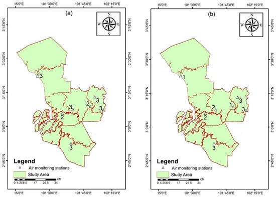
Figure 4.
The optimum order of the MC model for the observed (a) hourly and (b) daily API.

Figure 5.
The optimum order of the MC model for the simulated (a) hourly and (b) daily API.
4. Conclusions
In this study, the optimum order of the MC model for the hourly and daily API data, collected from seven stations in Peninsular Malaysia for a period of three years from 2012 to 2014, has been fitted in order to adequately represent the stochastic behavior of air pollution. The current study endeavors to shed some light on the intrinsic serial dependence of the hourly and daily API data through the proper choice of the MC model, based on the minimization of the BIC. The BIC has been used to determine the right order of the MC after testing the Markovian status with the chi-square test, based on the null hypothesis of serial independence. The log-likelihoods of the various orders of the MC have been determined and utilized to compute the BIC values. For the daily API, it is obvious that, according to the smallest values of BIC, the first-order MC is the most dominant in the stations. This is explained by the fact that the dependence of the concentration of the API on any given day is mainly reliant on a preceding day, and not on the long path via which that daily API is obtained. It can be also concluded from this study that the optimum order of the MC models for daily API occurrences varies from one station to another. It is observed that for both the observed and simulated hourly API, the second and the third order are more appropriate for most stations. This indicates that the API at any hour has dependence up to the previous two hours. In summary, this research might have significant implications for designing effective air quality management policies and promoting public health. In future work, the high-order multivariate MC model will be applied for modeling the sub-indexes of the API and some climatic factors, such as wind speed, temperature, and rainfall, in order to provide a comprehensive investigation of air pollution in the main cities of Malaysia. In addition, the MLE used in this study has a limitation in capturing the zero frequencies in the count matrices. According to this, future work should address this limitation by using a robust empirical Bayes method and conducting a simulation study based on the MCMC method to evaluate the model performance.
Author Contributions
Project administration, Y.A.; supervision, K.I., W.Z.W.Z. and M.O.; coding, Y.A. and N.V.; reviewing, K.I., W.Z.W.Z., N.V., M.O. and A.A.-Y. All authors have read and agreed to the published version of the manuscript.
Funding
This research was funded by the YUTP cost center, grant number (015LC0-296).
Institutional Review Board Statement
Not applicable.
Informed Consent Statement
Not applicable.
Data Availability Statement
The datasets generated and analyzed during the current study are not publicly available because they are confidential datasets, provided by the Department of Environment Malaysia, but they are available from the corresponding author on reasonable request.
Acknowledgments
The authors greatly appreciate the Department of Environment Malaysia and the Institute of Climate Change (IPI) and the Earth Observation Center (EOC) at Universiti Kebangsaan Malaysia for providing the air pollution data and the shapefile dataset that made this paper possible.
Conflicts of Interest
The authors declare that they have no conflict of interest.
References
- Manisalidis, I.; Elisavet, S.; Agathangelos, S.; Eugenia, B. Environmental and health impacts of air pollution: A review. Front. Public Health 2020, 8, 14. [Google Scholar] [CrossRef] [PubMed]
- Puentes, R.; Marchant, C.; Leiva, V.; Figueroa-Zúñiga, J.I.; Ruggeri, F. Predicting PM2.5 and PM10 levels during critical episodes management in Santiago, Chile, with a bivariate Birnbaum-Saunders log-linear model. Mathematics 2021, 9, 645. [Google Scholar] [CrossRef]
- Othman, J.; Sahani, M.; Mahmud, M.; Ahmad, M.K.S. Transboundary smoke haze pollution in Malaysia: Inpatient health impacts and economic valuation. Environ. Pollut. 2014, 189, 194–201. [Google Scholar] [CrossRef]
- Gass, K.; Klein, M.; Sarnat, S.E.; Winquist, A.; Darrow, L.A.; Flanders, W.D.; Chang, H.H.; Mulholland, J.A.; Tolbert, P.E.; Strickland, M.J. Associations between ambient air pollutant mixtures and pediatric asthma emergency department visits in three cities: A classification and regression tree approach. Environ. Health 2015, 14, 1–14. [Google Scholar] [CrossRef] [PubMed]
- Sun, D.; Li, X. Application of Markov chain model on environmental fate of phenanthrene in soil and groundwater. Procedia Environ. Sci. 2010, 2, 814–823. [Google Scholar] [CrossRef][Green Version]
- Zhou, Y.; Wang, L.; Zhong, R.; Tan, Y. A Markov chain based demand prediction model for stations in bike sharing systems. Math. Probl. Eng. 2018, 2018, 1–8. [Google Scholar] [CrossRef]
- Choji, D.N.; Eduno, S.N.; Kassem, G.T. Markov chain model application on share price movement in stock market. Comput. Eng. Intell. Syst. 2013, 4, 84–95. [Google Scholar]
- Saad, S.A.; Adnan, F.A.; Ibrahim, H.; Rahim, R. Manpower planning using Markov Chain model. In Proceedings of the AIP Conference Proceedings, Penang, Malaysia, 6–8 November 2013; AIP: College Park, MD, USA, 2014; pp. 1123–1127. [Google Scholar]
- Salas-Páez, C.; Quintana-Romero, L.; Mendoza-González, M.A.; Álvarez-García, J. Analysis of Job Transitions in Mexico with Markov Chains in Discrete Time. Mathematics 2022, 10, 1693. [Google Scholar] [CrossRef]
- Sahin, A.D.; Sen, Z. First-order Markov chain approach to wind speed modelling. J. Wind. Eng. Ind. Aerodyn. 2001, 89, 263–269. [Google Scholar] [CrossRef]
- Shamshad, A.; Bawadi, M.; Hussin, W.W.; Majid, T.A.; Sanusi, S. First and second order Markov chain models for synthetic generation of wind speed time series. Energy 2005, 30, 693–708. [Google Scholar] [CrossRef]
- Fawcett, L.; Walshaw, D. Markov chain models for extreme wind speeds. Env. Off. J. Int. Env. Soc. 2006, 17, 795–809. [Google Scholar] [CrossRef]
- Carpinone, A.; Giorgio, M.; Langella, R.; Testa, A. Markov chain modeling for very-short-term wind power forecasting. Electr. Power Syst. Res. 2015, 122, 152–158. [Google Scholar] [CrossRef]
- Larsen, L.; Bradley, R.; Honcoop, G. A new method of characterizing the variability of air quality-related indicators. In Proceedings of the Air and waste management association’s international specialty conference of tropospheric ozone and the environment, Los Angeles, CA, USA, 3 May 1990. [Google Scholar]
- Hoyos, L.; Lara, P.; Ortiz, E.; Bracho, R.L.; González, J. Evaluation of air pollution control policies in Mexico City using finite Markov chain observation model. Rev. Matemática Teoría Apl. 2009, 16, 255–266. [Google Scholar] [CrossRef][Green Version]
- Rodrigues, E.R.; Achcar, J.A. Applications of Discrete-Time Markov Chains and Poisson Processes to Air Pollution Modeling and Studies; Springer Science & Business Media: Berlin/Heidelberg, Germany, 2012. [Google Scholar]
- Asadollahfardi, G.; Zangooei, H.; Aria, S.H. Predicting PM 2.5 concentrations using artificial neural networks and Markov chain, a case study Karaj City. Asian J. Atmos. Environ. 2016, 10, 67–79. [Google Scholar] [CrossRef]
- Nebenzal, A.; Fishbain, B. Long-term forecasting of nitrogen dioxide ambient levels in metropolitan areas using the discrete-time Markov model. Environ. Model. Softw. 2018, 107, 175–185. [Google Scholar] [CrossRef]
- Mohamad, N.; Deni, S.; Ul-Saufie, A. Application of the First Order of Markov Chain Model in Describing the PM10 Occurrences in Shah Alam and Jerantut, Malaysia. Pertanika J. Sci. Technol. 2018, 26, 367–378. [Google Scholar]
- Alyousifi, Y.; Masseran, N.; Ibrahim, K. Modeling the stochastic dependence of air pollution index data. Stoch. Environ. Res. Risk Assess. 2018, 32, 1603–1611. [Google Scholar] [CrossRef]
- Alyousifi, Y.; Ibrahim, K.; Kang, W.; Zin, W.Z.W. Markov chain modeling for air pollution index based on maximum a posteriori method. Air Qual. Atmos. Health 2019, 12, 1521–1531. [Google Scholar] [CrossRef]
- Chen, J.-C.; Wu, Y.J. Discrete-time Markov chain for prediction of air quality index. J. Ambient. Intell. Humaniz. Comput. 2020, 9, 1–10. [Google Scholar] [CrossRef]
- Alyousifi, Y.; Ibrahim, K.; Kang, W.; Zin, W.Z.W. Modeling the spatio-temporal dynamics of air pollution index based on spatial Markov chain model. Environ. Monit. Assess. 2020, 192, 1–24. [Google Scholar]
- Tijms, H.C. A First Course in Stochastic Models; John Wiley and Sons: Hoboken, NJ, USA, 2003. [Google Scholar]
- Ching, W.-K.; Huang, X.; Ng, M.K.; Siu, T.-K. Higher-order markov chains. In Markov Chains; Springer: Berlin/Heidelberg, Germany, 2013; pp. 141–176. [Google Scholar]
- Ibe, O. Markov Processes for Stochastic Modeling; Newnes: Oxford, UK, 2013. [Google Scholar]
- Privault, N. Understanding markov chains. Ex. Appl. Publ. 2013, 357, 358. [Google Scholar]
- Grinstead, C.M.; Snell, J.L. Introduction to Probability; American Mathematical Soc.: Providence, RI, USA, 1997. [Google Scholar]
- Nikolić, D.; Milošević, N.; Mihajlović, I.; Živković, Ž.; Tasić, V.; Kovačević, R.; Petrović, N. Multi-criteria analysis of air pollution with SO2 and PM10 in urban area around the copper smelter in Bor, Serbia. Water Air Soil Pollut. 2010, 206, 369–383. [Google Scholar] [CrossRef] [PubMed][Green Version]
- Li, C.-K.; Zhang, S. Stationary probability vectors of higher-order Markov chains. Linear Algebra Its Appl. 2015, 473, 114–125. [Google Scholar] [CrossRef]
- Anderson, T.W.; Goodman, L.A. Statistical inference about Markov chains. Ann. Math. Stat. 1957, 28, 89–110. [Google Scholar] [CrossRef]
- Billingsley, P. Statistical methods in Markov chains. Ann. Math. Stat. 1961, 32, 12–40. [Google Scholar] [CrossRef]
- Katz, R.W. On some criteria for estimating the order of a Markov chain. Technometrics 1981, 23, 243–249. [Google Scholar] [CrossRef]
- Deni, S.M.; Jemain, A.A.; Ibrahim, K. Fitting optimum order of Markov chain models for daily rainfall occurrences in Peninsular Malaysia. Theor. Appl. Climatol. 2009, 97, 109–121. [Google Scholar] [CrossRef]
- Bickenbach, F.; Bode, E. Evaluating the Markov property in studies of economic convergence. Int. Reg. Sci. Rev. 2003, 26, 363–392. [Google Scholar] [CrossRef]
- Skuriat-Olechnowska, M. Statistical inference and hypothesis testing for Markov chains with Interval Censoring. Master’s Thesis, Delft University of Technology, Delft, The Netherlands, 2005. [Google Scholar]
- Spedicato, G. A package to handle and analyse discrete time Markov Chains. R Package Version 2014, 95, 1–17. [Google Scholar]
- Bickenbach, F.; Bode, E. Markov or Not Markov-This Should Be a Question; Kiel working paper; Kiel Institute of World Economics: Kiel, Germany, 2001. [Google Scholar]
- Schoof, J.; Pryor, S. On the proper order of Markov chain model for daily precipitation occurrence in the contiguous United States. J. Appl. Meteorol. Climatol. 2008, 47, 2477–2486. [Google Scholar] [CrossRef]
- Jimoh, O.; Webster, P. The optimum order of a Markov chain model for daily rainfall in Nigeria. J. Hydrol. 1996, 185, 45–69. [Google Scholar] [CrossRef]
- Mohamad, N.; Deni, S.; Japeri, A. Modeling of daily PM10 concentration occurrence using Markov Chain model in Shah Alam, Malaysia. J. Environ. Sci. Technol. 2017, 10, 96–106. [Google Scholar] [CrossRef]
- Dastidar, A.G.; Ghosh, D.; Dasgupta, S.; De, U. Higher order Markov chain models for monsoon rainfall over West Bengal, India. Indian J. Radio Space Phys. 2010, 39, 39–44. [Google Scholar]
- Wilks, D.S. Statistical Methods in the Atmospheric Sciences; Academic Press: London, UK, 2011; Volume 100. [Google Scholar]
- Bowerman, B.L.; O’Connell, R.T.; Koehler, A.B. Forecasting, Time Series, and Regression: An Applied Approach; South-Western Pub: San Diego, CA, USA, 2005; Volume 4. [Google Scholar]
- Masseran, N.; Safari, M.A.M. Modeling the transition behaviors of PM10 pollution index. Environ. Monit. Assess. 2020, 192, 1–15. [Google Scholar] [CrossRef] [PubMed]
- Chin, S.A. A relativistic many-body theory of high density matter. Ann. Phys. 1977, 108, 301–367. [Google Scholar] [CrossRef]
- World Health Organization. Air Quality Guidelines for Europe; World Health Organization, Regional Office for Europe: Geneva, Switzerland, 2000. [Google Scholar]
- Barbu, V.S.; Bérard, C.; Cellier, D.; Sautreuil, M.; Vergne, N. SMM: An R Package for Estimation and Simulation of Discrete-time semi-Markov Models. R J. 2018, 10, 226. [Google Scholar] [CrossRef]
- Vergne, N. Drifting Markov models with polynomial drift and applications to DNA sequences. Stat. Appl. Genet. Mol. Biol. 2008, 7, 6. [Google Scholar] [CrossRef]
- Barbu, V.S.; Vergne, N. Reliability and survival analysis for drifting Markov models: Modeling and estimation. Methodol. Comput. Appl. Probab. 2019, 21, 1407–1429. [Google Scholar] [CrossRef]
Publisher’s Note: MDPI stays neutral with regard to jurisdictional claims in published maps and institutional affiliations. |
© 2022 by the authors. Licensee MDPI, Basel, Switzerland. This article is an open access article distributed under the terms and conditions of the Creative Commons Attribution (CC BY) license (https://creativecommons.org/licenses/by/4.0/).