Optimal Pension Fund Management with Foreign Investment in a Stochastic Environment

Abstract

To ensure the success of a pension plan under a self-contained defined contribution (DC) retirement plan, the inclusion of foreign assets in a local pension portfolio could be beneficial for risk diversification and the efficient improvement of a fund’s investment performance during its accumulation phase. This study focuses on developing international asset allocation criteria for a DC pension plan; accordingly, we consider risk exposure relative to stochastic interest rates and ex- change rates with minimum guarantees. An arbitrage-free framework, namely, the cross-currency Heath–Jarrow–Morton interest rate model, is introduced in dynamic optimization programming for the DC pension fund. The proposed solution based on the generalized stochastic framework provides tractable and appropriate criteria for the dynamic allocation of a DC pension fund. The constituents of the optimal solution can reflect changes in investment lifecycles and shifts in risk preferences during the accumulation phase of a DC pension plan.

1. Introduction

With societal aging and an increase in the number of retirees in developed nations, the success of a pension fund may depend on whether sufficient wealth is accumulated through contributions and investment to satisfy an individual’s financial needs during retirement. A defined benefit (DB) plan, one of two types of pension plans, may allow contributors to bear a low financial risk from uncertainties during the accumulation phase. In a DB plan, the final benefits to contributors are fixed, although periodic contributions are random in the distribution phase. A defined contribution (DC) plan, by contrast, exposes contributors to substantial financial risk in both the accumulation and distribution phases because it operates under a stochastic model. In a DC plan, contributors hold savings management accounts, and the benefits to participants are uncertain. Such benefits mainly depend on the performance of investment funds during the distribution phase.

To ensure the success of a self-contained DC pension plan, foreign assets may be included in pension portfolios because such assets ensure risk diversification and efficient frontier improvement [1]. As an economy matures, restrictions on foreign asset investments in pension schemes are often reduced [2]. Research on pension plan optimization based on minimum guarantees of terminal annuity payoffs has increased in the literature [3] and other related works [4,5,6,7]; researchers endeavor to develop theoretical frameworks for pension plan optimization.

However, none of the studies in the literature consider including foreign assets, stochastic interest rates, and exchange rates altogether in retirement portfolios. Discussions of strategies for domestic and foreign asset allocation as well as for hedging against foreign exchange risks are limited. For example, the most relevant studies develop allocative criteria by making postulations about the contributions of domestic assets such as stocks, bonds, cash [5,6,8], or commodities [9]. Recently, researchers attempted to solve stochastic dynamic programming problems by considering conventional and nonconventional risk sources in the context of interest rate and security risks. For example, the literature in [10,11] consider inflation-related risks for pension plan optimization.

Once a domestic pension fund is no longer subject to capital constraints and such capital can move freely both domestically and internationally, the differences between local and foreign assets should not be ignored; attention should be given to the complications associated with such assets during the allocative optimization process. On the basis of the stochastic dynamic programming framework proposed by [12,13], we expect that the portfolio performance of a local pension fund permitted to conduct foreign investments would depend on assets’ risk–return characteristics and on the exchange rate for foreign assets.

To consider the dynamics of asset price paths related to both domestic and foreign currencies, this study introduces a cross-currency Heath–Jarrow–Morton (HJM) model. This model is based on the model in the literature [14] for stochastic dynamic programming related to DC plan optimization. The cross-currency HJM model is an extension of the HJM forward rate model proposed in 1987 and formally published in 1992 [15]. The cross-currency HJM model developed in [14] is mainly used for pricing foreign currency options. In this study, that model is applied in the context of DC pension plans to construct an alternative stochastic dynamic programming model under which the price dynamics of both domestic and foreign assets can be reflected.

The related literature mostly focuses on the field of dynamic asset allocation; in this context, the corresponding decision criteria are derived using a market equilibrium interest rate framework (the short rate model), such as the [16] Vasicek (1977) model [3,6,8,11,17], the [18] CIR (1985) framework [10,19], or an analogously general affine model [5] for algorithm convenience. However, the market equilibrium model has at least two obvious defects. First, the model may lead to interest rates having an unreasonable term structure. For example, applying the Vasicek model may result in negative interest rates; this situation is not in line with real-world scenarios. Second, the model is not suitable for tasks aimed at capturing the practical term structure of interest rates. The market equilibrium model was developed on the basis of an ideal market equilibrium status; thus, the short rates derived using this model are abstract and unobservable in real-world markets. Specifically, the developed term structure of interest rates under the equilibrium model usually fails to fit the actual paths of interest rates in real-world settings.

In the arbitrage-free model, the corresponding term structure of interest rates is typically developed using a martingale measure, in which transactions are treated as a fair game; thus, constructing an arbitrage profit model using two or more of those prices is impractical. Arbitrage-free models such as the [15] HJM (1992) model are developed in the field of financial derivatives pricing [20] because such models are sufficiently flexible for describing the effects of complex dynamic features (e.g., nonconstant volatility and correlations) or dependence structures on the state space of forward rate curves. Forward rate curves embed all information on default-free bond prices; only volatilities in their dynamic paths need to be estimated. To overcome the limitations of the equilibrium model, this study presents an HJM-model–based interest rate model; this model constitutes an efficient martingale approach for solving the stochastic dynamic programming problem for DC pension plans in real-world contexts.

The rest of this article is organized as follows. The next section introduces the technical aspects and assumptions for describing the dynamics of assets in a two-country economy. The Section 3 demonstrates how the dynamic programming model and formulae for optimal asset allocations of a DC pension plan are constructed in a stochastic environment. Numerical analyses based on the developed decision criteria and the experimental results are described in the Section 4. Finally, the Section 5 provides the conclusions.

2. Economy and Model

2.1. Stochastic Environment and the Two-Country Model

Consider a complete financial market in a real-world setting without arbitrage or friction; in this continuously open environment, trading occurs continuously over the time interval $\left[0,\mathcal{T}\right]$, where $0<\mathcal{T}<\infty$. The uncertainty is described by the filtered probability space $\left(\Omega ,\mathcal{F},\mathbb{P},{\left\{{\mathcal{F}}_t\right\}}_{t\in \left[0,\mathcal{T}\right]}\right)$, where $\mathbb{P}$ is the real-world probability and $\mathcal{F}={\left\{{\mathcal{F}}_t\right\}}_{t\in \left[0,\mathcal{T}\right]}$ is the filtration generated by an n-dimensional, independent, standard Brownian motion vector $\tilde{\mathit{W}}\left(t\right)={[W_1\left(t\right),W_2\left(t\right),\dots ,W_n\left(t\right)]}^{\prime }$; the n × 1 vector, $\tilde{\mathit{W}}\left(t\right)$, represents n random shocks or the aforementioned idiosyncratic risks in the market. For local investors other than those in the United States, foreign assets are mostly denominated in US dollars. For simplicity and to ensure that exchange rate risks are included, the market is considered to be a real-world two-country economy. A DC pension plan can flexibly allocate cash assets (money market account, MMA), zero-coupon bonds (ZCBs), and stock portfolios, all of which are denominated in domestic and foreign currencies for dealing with exchange rate, interest rate, and security risks, respectively. The subscripts $d$ and $f$ represent domestic and foreign assets, respectively.

• $M_k\left(t\right)$ = the time t value of the k-th country’s cash asset, with its initial value $M_k\left(0\right)=1$ being a unit of the k-th currency for k $\in \left\{d,f\right\}$.
• $f_k\left(t,T\right)$ = the k-th country’s instantaneous forward interest rate contracted at time t but effective at time T where $0\le t\le T\le \mathcal{T}$.
• $r_k\left(t\right)$ = $f_k\left(t,t\right),$ the k-th country’s instantaneous risk-free short rate at time t.
• $B_k\left(t,T\right)$ = $\exp \left(-{{\displaystyle \int }}_t^T{f}_k(t,u)du\right)$ the time t price in the k-th country’s currency for a ZCB paying one unit of the k-th currency at maturity T.
• $S_k\left(t\right)$ = the time t price in the k-th currency for the k-th country’s stock portfolio.
• $X\left(t\right)$ = the exchange rate spot price at time t for one unit of foreign currency.
• $M_f^{*}\left(t\right)$ = $M_f\left(t\right)X\left(t\right)$, the time t domestic value of foreign cash assets.
• $B_f^{*}\left(t,T\right)$ = $B_f\left(t,T\right)X\left(t\right)$, the time t domestic value of a foreign ZCB for one unit of foreign currency at its maturity T.
• $S_f^{*}\left(t\right)$ = $S_f\left(t\right)X\left(t\right)$, the time t price of a foreign stock portfolio denominated in domestic currency.

According to the basic frameworks presented by [14,21], the related and extended conditions that describe the asset dynamics in the market are described in the following assumptions.

Assumption 1.

The dynamics of a cash asset are as follows:

$$\frac{d{M}_k\left(t\right)}{M_k\left(t\right)}=r_k\left(t\right)dt, M_k\left(0\right)=1\hspace{1em};\hspace{1em}\mathrm{for} k\in \left\{d,f\right\}.$$

(1)

Thus, the price of the k-th country’s cash asset at time t is expressed as$M_k\left(t\right)=exp\left({{\displaystyle \int }}_0^t{r}_k\left(u\right)du\right)$, where$r_k\left(t\right)$is the time t instantaneous riskless rate of interest of the k-th country.

Assumption 2.

The evolvement process for the T-maturity forward rate, which is derived from an extension of the [15] HJM (1992) model under the real-world probability measure $\mathbb{P}$, is described as follows:

$$d{f}_k\left(t,T\right)={\alpha }_k\left(t,T\right)dt-{\tilde{\mathit{\sigma }}}_k{\left(t,T\right)}^{\prime }d\tilde{\mathit{W}}\left(t\right) ; k\in \left\{d,f\right\}$$

(2)

where ${\alpha }_k\left(t,T\right)$ represents the drift term and ${\tilde{\mathit{\sigma }}}_k\left(t,T\right)={\left[{\sigma }_{k1}\left(t,T\right),\dots ,{\sigma }_{kn}\left(t,T\right)\right]}^{\prime }$, $k\in \left\{d,f\right\}$, a diffusion vector, represents an $n\times 1$ vector of deterministic functions of time. Both ${\alpha }_k\left(t,T\right)$ and ${\tilde{\mathit{\sigma }}}_k\left(t,T\right)$ satisfy some regular conditions.

On the basis of the multifactor HJM (1992) framework [15] in Equation (2), the dynamics of ZCBs can be derived from the following proposition:

Proposition 1

(Price process of a T-maturity ZCB under the HJM model). The dynamics of a T−maturity ZCB under the HJM (1992) framework and real-world probability measure$\mathbb{P}$can be derived as follows:

$$\frac{d{B}_k\left(t,T\right)}{B_k\left(t,T\right)}=\left[r_k\left(t\right)+b_k\left(t,T\right)\right]dt+{\tilde{\mathit{\nu }}}_k{\left(t,T\right)}^{\prime }d\tilde{\mathit{W}}\left(t\right) ; k\in \left\{d,f\right\}$$

(3)

with

$$\begin{array}{c}{b}_k\left(t,T\right)=\left[-a_k\left(t,T\right)+\frac{1}{2}\Vert {\tilde{\mathit{\nu }}}_k\left(t,T\right){\Vert }^2\right]\\ a_k\left(t,T\right)={{\displaystyle \int }}_t^T{\alpha }_k\left(t,u\right)du\\ {\tilde{\mathit{\nu }}}_k\left(t,T\right)={{\displaystyle \int }}_t^T{\tilde{\mathit{\sigma }}}_k\left(t,u\right)du\end{array}$$

where${\tilde{\mathit{\nu }}}_k\left(t,T\right)={[{{\displaystyle \int }}_t^T{\sigma }_{k1}\left(t,u\right)du,\dots ,{{\displaystyle \int }}_t^T{\sigma }_{kn}\left(t,u\right)du]}^{\prime }$, is an$n\times 1$volatility vector for$k\in \left\{d,f\right\}$.

Proof of Proposition 1.

See [15] HJM (1992) for details. □

It could be unrealistic to assume that a ZCB exists whose maturity exactly matches the retirement date for a pension plan. Relative to the whole investment horizon T of a pension plan, only market-tradable ZCBs with short maturities might be obtainable. On the basis of the models presented by [3,22], the aforementioned model further introduces a bond portfolio and dynamically adjusts its components to retain a constant duration $\tau \in \left(0,T\right]$; such a bond is known as a rolling bond. Because a rolling bond with a short constant duration $\tau \in \left(0,T\right]$ is easily obtainable in practice, the fund optimization for ZCBs is executed in terms of rolling ZCBs rather than their T-maturity counterparts. The dynamics of a rolling ZCB can be specified as follows:

Assumption 3.

Given an arbitrary constant maturity$\tau \in \left(0,T\right]$, the time$t$value of a rolling ZCB$\left(B_k^{\tau }\left(t\right)\right)$is expressed as follows:

$$\frac{d{B}_k^{\tau }\left(t\right)}{B_k^{\tau }\left(t\right)}=\left[r_k\left(t\right)+b_k^{\tau }\left(t\right)\right]dt+{\tilde{\mathit{\nu }}}_k^{\tau }{\left(t\right)}^{\prime }d\tilde{\mathit{W}}\left(t\right) ; k\in \left\{d,f\right\}$$

(4)

where${\tilde{\mathit{\nu }}}_k^{\tau }\left(t\right)=\left[{{\displaystyle \int }}_t^{t+\tau }{\sigma }_{k1}\left(t,u\right)du,\dots ,{{\displaystyle \int }}_t^{t+\tau }{\sigma }_{kn}\left(t,u\right)du\right]$, and$b_k^{\tau }\left(t\right)=\left[-a_k^{\tau }\left(t\right)+\frac{1}{2}\Vert {\tilde{\mathit{\nu }}}_k^{\tau }\left(t\right){\Vert }^2\right]$with$a_k^{\tau }\left(t\right)={{\displaystyle \int }}_t^{t+\tau }{\alpha }_k\left(t,u\right)du$for$k\in \left\{d,f\right\}$.

In the described pension plan optimization procedure, a stock portfolio is considered, and its dynamics related to the real-world probability measure $\mathbb{P}$ can be described as follows:

Assumption 4.

The price paths of a stock asset under the real-world probability measure$\mathbb{P}$can be expressed as follows:

$$\frac{d{S}_k\left(t\right)}{S_k\left(t\right)}={\mu }_{sk}\left(t\right)dt+{\tilde{\mathit{\sigma }}}_{sk}{\left(t\right)}^{\prime }d\tilde{\mathit{W}}\left(t\right) ; k\in \left\{d,f\right\}$$

(5)

where${\mu }_{sk}\left(t\right)$is${\mathcal{F}}_t$-adapted and${\tilde{\mathit{\sigma }}}_{sk}\left(t\right)={\left[{\sigma }_{sk,1}\left(t\right),\dots ,{\sigma }_{sk,n}\left(t\right)\right]}^{\prime }$is an$n\times 1$vector of deterministic functions of time. Both${\mu }_{sk}\left(t\right)$and${\tilde{\mathit{\sigma }}}_{sk}\left(t\right)$satisfy some technical smoothness and boundedness conditions.

2.2. Dynamics of Foreign Assets in a Domestic Currency Context

In our two-country model, the link facilitating trade between the two economies is facilitated by the spot exchange rate, whose dynamics are assumed to follow a geometric Brownian motion.

Assumption 5.

The dynamics of an exchange rate under$\mathbb{P}$are as follows:

$$\frac{dX\left(t\right)}{X\left(t\right)}={\mu }_X\left(t\right)dt+{\tilde{\mathit{\sigma }}}_X{\left(t\right)}^{\prime }d\tilde{\mathit{W}}\left(t\right)$$

(6)

where${\mu }_X\left(t\right)$is${\mathcal{F}}_t$-adapted and${\tilde{\mathit{\sigma }}}_X\left(t\right)={\left[{\sigma }_{X1}\left(t\right),\dots ,{\sigma }_{Xn}\left(t\right)\right]}^{\prime }$is an$n\times 1$vector of deterministic functions of time. Both of them satisfy some smoothness and boundedness conditions, which are analogous to the previous setting, for consequent derivation.

Because a pension portfolio ensures asset optimization from a domestic trader–based perspective, we must convert foreign assets to a domestic currency; this can be achieved by multiplying the spot exchange rate by such foreign assets. The domestic value of these foreign assets, including cash, ZCBs, and stock portfolios, is then denominated; the related dynamics can be accordingly derived using Itô’s lemma.

Corollary 1

(Dynamics of foreign assets in a domestic currency context). The dynamics of domestic-currency-denominated foreign assets are specified as follows:

$$\frac{d{M}_f^{*}\left(t\right)}{M_f^{*}\left(t\right)}=\left[r_f\left(t\right)+{\mu }_X\left(t\right)\right]dt+{\tilde{\mathit{\sigma }}}_X{\left(t\right)}^{\prime }d\tilde{\mathit{W}}\left(t\right)$$

(7)

$$\frac{d{B}_f^{*}\left(t,T\right)}{B_f^{*}\left(t,T\right)}=\left[r_f\left(t\right)+b_f\left(t,T\right)+{\mu }_X\left(t\right)+{\tilde{\mathit{\nu }}}_f{\left(t,T\right)}^{\prime }{\tilde{\mathit{\sigma }}}_X\left(t\right)\right]dt+{\left[{\tilde{\mathit{\nu }}}_f\left(t,T\right)+{\tilde{\mathit{\sigma }}}_X\left(t\right)\right]}^{\prime }d\tilde{\mathit{W}}\left(t\right)$$

(8)

$$\frac{d{B}_f^{*\tau }\left(t\right)}{B_f^{*\tau }\left(t\right)}=\left[r_f\left(t\right)+b_f^{\tau }\left(t\right)+{\mu }_X\left(t\right)+{\tilde{\mathit{\nu }}}_f^{\tau }{\left(t\right)}^{\prime }{\tilde{\mathit{\sigma }}}_X\left(t\right)\right]dt+{\left[{\tilde{\mathit{\nu }}}_f^{\tau }\left(t\right)+{\tilde{\mathit{\sigma }}}_X\left(t\right)\right]}^{\prime }d\tilde{\mathit{W}}\left(t\right)$$

(9)

$$\frac{d{S}_f^{*}\left(t\right)}{S_f^{*}\left(t\right)}=\left[{\mu }_{sf}\left(t\right)+{\mu }_X\left(t\right)+{\tilde{\mathit{\sigma }}}_{sf}{\left(t\right)}^{\prime }{\tilde{\mathit{\sigma }}}_X\left(t\right)\right]dt+{\left[{\tilde{\mathit{\sigma }}}_{sf}\left(t\right)+{\tilde{\mathit{\sigma }}}_X\left(t\right)\right]}^{\prime }d\tilde{\mathit{W}}\left(t\right)$$

(10)

Equation (9) presents the dynamics of a foreign rolling bond with a shorter constant$\tau$−maturity; this bond is denominated in domestic currency.

2.3. Existence and Uniqueness of the Market Price of Risk

Because the market in a two-economy framework is arbitrage-free and complete, n, which is equal to (dn + fn + 3) dimensions of risks, can be replicated (hedged) by n distinct market assets. The n distinct risky assets include domestic and foreign ZCBs with different dn and fn maturities, respectively; a stock portfolio in both domestic and foreign markets; and a foreign cash asset. Similar to the derivations in the related literature [14,15,21], in this study, the n risky assets accompanying a domestic cash asset are combined to ensure that a unique set of market prices of risks arising from the corresponding market risks can be determined through the following proposition:

Proposition 2

(Uniqueness and existence of the market prices of risks). Given arbitrary different dn domestic ZCBs with constant maturities$\{{\tau }_{d1}<\cdots <{\tau }_{dn}\}\in \left(0,\mathcal{T}\right]$, different fn foreign ZCBs with constant maturities$\{{\tau }_{f1}<\cdots <{\tau }_{fn}\}\in \left(0,\mathcal{T}\right]$, a corresponding spot exchange rate, and a stock portfolio in both domestic and foreign stock markets, there exists a unique set of time-deterministic solutions$\tilde{\mathit{\lambda }}={\left\{{\lambda }_i\right\}}_{i=1,\dots ,n}$for the market prices of risks if the following equation set is satisfied.

$$\left[\begin{array}{c}{b}_d^{{\tau }_{d1}}\left(t\right)\\ ⋮\\ b_d^{{\tau }_{dn}}\left(t\right)\\ {\mu }_{sd}\left(t\right)-r_d\left(t\right)\\ r_f\left(t\right)+{\mu }_X\left(t\right)-r_d\left(t\right)\\ r_f\left(t\right)+{\mu }_X\left(t\right)+b_f^{{\tau }_{f1}}\left(t\right)+{\tilde{\mathit{\nu }}}_f^{{\tau }_{f1}}{\left(t\right)}^{\prime }{\tilde{\mathit{\sigma }}}_X\left(t\right)-r_d\left(t\right)\\ ⋮\\ r_f\left(t\right)+{\mu }_X\left(t\right)+b_f^{{\tau }_{fn}}\left(t\right)+{\tilde{\mathit{\nu }}}_f^{{\tau }_{fn}}{\left(t\right)}^{\prime }{\tilde{\mathit{\sigma }}}_X\left(t\right)-r_d\left(t\right)\\ {\mu }_X\left(t\right)+{\mu }_{sf}\left(t\right)+{\tilde{\mathit{\sigma }}}_{sf}{\left(t\right)}^{\prime }{\tilde{\mathit{\sigma }}}_X\left(t\right)-r_d\left(t\right)\end{array}\right]-\left[\begin{array}{c}{\tilde{\mathit{\nu }}}_d^{{\tau }_{d1}}\left(t\right){}^{\prime }\\ ⋮\\ {\tilde{\mathit{\nu }}}_d^{{\tau }_{dn}}\left(t\right){}^{\prime }\\ {\tilde{\mathit{\sigma }}}_{sd}\left(t\right){}^{\prime }\\ {\tilde{\mathit{\sigma }}}_X\left(t\right){}^{\prime }\\ \left({\tilde{\mathit{\nu }}}_f^{{\tau }_{f1}}\left(t\right)+{\tilde{\mathit{\sigma }}}_X\left(t\right)\right){}^{\prime }\\ ⋮\\ \left({\tilde{\mathit{\nu }}}_f^{{\tau }_{fn}}\left(t\right)+{\tilde{\mathit{\sigma }}}_X\left(t\right)\right){}^{\prime }\\ \left({\tilde{\mathit{\sigma }}}_{sf}\left(t\right)+{\tilde{\mathit{\sigma }}}_X\left(t\right)\right){}^{\prime }\end{array}\right]\left[\begin{array}{c}{\lambda }_{d1}\\ ⋮\\ {\lambda }_{dn}\\ {\lambda }_{sd}\\ {\lambda }_X\\ {\lambda }_{f1}\\ ⋮\\ {\lambda }_{fn}\\ {\lambda }_{sf}\end{array}\right]=\tilde{\mathbf{0}}$$

or equivalently

$$\tilde{\mathit{\Lambda }}-\mathit{\Gamma }\tilde{\mathit{\lambda }}=\tilde{\mathbf{0}}$$

(11)

where$\tilde{\mathit{\Lambda }}$is the$n\times 1$vector of the excess returns on risky assets and$\tilde{\mathbf{0}}$is an$n\times 1$vector of zeros. Because the market is arbitrage-free and complete, the$n\times n$volatility matrix$\mathit{\Gamma }$is nonsingular, guaranteeing a unique solution for solving$\tilde{\mathit{\lambda }}$. Therefore, the$n\times 1$vector of market prices of risks$\tilde{\mathit{\lambda }}$can be uniquely determined through Equation (11), whose i-th component is the market price of risk associated with$W_i\left(t\right)$, that is, the i-th Brownian motion.

Proof. 

Refer to [14,15,21] for the analogous details. □

Because of the existence and uniqueness of the market prices of risks, the dynamics of observable assets in a two-economy model, including cash, constant rolling bonds, and stocks, can be re-expressed in the form of market prices of risks presented in drifts.

Corollary 2

(Dynamics of domestic-currency-denominated assets with the market prices of risks).On the basis of the results in Proposition 2, the dynamics of assets denominated in the domestic currency in the two-economy model under the real-world probability measure$\mathbb{P}$can be re-expressed as follows:

$$\frac{d{B}_d^{\tau }\left(t\right)}{B_d^{\tau }\left(t\right)}=\left[r_d\left(t\right)+{\tilde{\mathit{\nu }}}_d^{\tau }{\left(t\right)}^{\prime }\tilde{\mathit{\lambda }}\right]dt+{\tilde{\mathit{\nu }}}_d^{\tau }{\left(t\right)}^{\prime }d\tilde{\mathit{W}}\left(t\right)$$

(12)

$$\frac{d{S}_d\left(t\right)}{S_d\left(t\right)}=\left[r_d\left(t\right)+{\tilde{\mathit{\sigma }}}_{sd}{\left(t\right)}^{\prime }\tilde{\mathit{\lambda }}\right]dt+{\tilde{\mathit{\sigma }}}_{sd}{\left(t\right)}^{\prime }d\tilde{\mathit{W}}\left(t\right)$$

(13)

$$\frac{d{M}_f^{*}\left(t\right)}{M_f^{*}\left(t\right)}=\left[r_d\left(t\right)+{\tilde{\mathit{\sigma }}}_X{\left(t\right)}^{\prime }\tilde{\mathit{\lambda }}\right]dt+{\tilde{\mathit{\sigma }}}_X{\left(t\right)}^{\prime }d\tilde{\mathit{W}}\left(t\right)$$

(14)

$$\frac{d{B}_f^{*\tau }\left(t\right)}{B_f^{*\tau }\left(t\right)}=\left[r_d\left(t\right)+{\left({\tilde{\mathit{\nu }}}_f^{\tau }\left(t\right)+{\tilde{\mathit{\sigma }}}_X\left(t\right)\right)}^{\prime }\tilde{\mathit{\lambda }}\right]dt+{\left[{\tilde{\mathit{\nu }}}_f^{\tau }\left(t\right)+{\tilde{\mathit{\sigma }}}_X\left(t\right)\right]}^{\prime }d\tilde{\mathit{W}}\left(t\right)$$

(15)

$$\frac{d{S}_f^{*}\left(t\right)}{S_f^{*}\left(t\right)}=\left[r_d\left(t\right)+{\left({\tilde{\mathit{\sigma }}}_{sf}\left(t\right)+{\tilde{\mathit{\sigma }}}_X\left(t\right)\right)}^{\prime }\tilde{\mathit{\lambda }}\right]dt+{\left[{\tilde{\mathit{\sigma }}}_{sf}\left(t\right)+{\tilde{\mathit{\sigma }}}_X\left(t\right)\right]}^{\prime }d\tilde{\mathit{W}}\left(t\right)$$

(16)

$$\frac{dX\left(t\right)}{X\left(t\right)}=\left[r_d\left(t\right)-r_f\left(t\right)+{\tilde{\mathit{\sigma }}}_X{\left(t\right)}^{\prime }\tilde{\mathit{\lambda }}\right]dt+{\tilde{\mathit{\sigma }}}_X{\left(t\right)}^{\prime }d\tilde{\mathit{W}}\left(t\right)$$

(17)

If foreign assets are not considered in a pension portfolio, then the asset dynamics in Equations (14)–(17), all of which involve exchange rate uncertainty, are irrelevant in allocative optimization. The two-economy model can thus be easily simplified as a conventional optimization problem, which has been examined by several research groups [3,17,23]; these researchers mainly focus on pension portfolio optimization in the context of conventional domestic assets.

In an extended two-economy model, the evolution of risky assets reflects the influences of and interactions between all uncertainties in markets because all the random shocks $\tilde{\mathit{W}}\left(t\right)={\left\{W_i\right\}}_{i=1,\dots ,n}$ from different risk sources are considered in the corresponding components of their diffusion terms. Thus, the evolution of the term structure of instantaneous forward interest rates and the corresponding bond assets are established on the basis of the multifactor HJM framework. Under the given condition and proposition, we can now deal with the optimization problem for a DC pension scheme in the context of stochastic interest rates and a minimum guaranteed payment.

3. Allocative Optimization for a DC Pension Scheme

3.1. Contribution Flow, Wealth Process, and Contingent Claim

Under the continuous-time formulation for a DC pension scheme, an annuitant continuously contributes to their pension fund before their retirement date T. The contribution process with respect to contemporary salaries is stochastic [6,10].

Assumption 6.

The contribution process for a DC pension is stochastic and can be expressed as follows:

$$\frac{dC\left(t\right)}{C\left(t\right)}={\mu }_{C}dt+{\tilde{\mathit{\sigma }}}_C{\left(t\right)}^{\prime }d\tilde{\mathit{W}}\left(t\right)$$

(18)

where the volatility${\tilde{\mathit{\sigma }}}_C\left(t\right)={\left[{\sigma }_{C,1}\left(t\right),\dots ,{\sigma }_{C,dn},{\sigma }_{C,dn+1},0,\dots ,0\right]}^{\prime }$is an$n\times 1$vector with the first$\left(dn+1\right)$nonzero entries, which reflects the sources of domestic risk factors. Furthermore, the volatility vector is a deterministic function of time subject to the technical smoothness and boundedness condition${{\displaystyle \int }}_0^T{\sigma }_{Ci}^2\left(t\right)dt<\infty ,$$\forall i=1,\dots ,n$for its entries.

Because the contribution rate ${\mu }_C$ is intuitively related to domestic salaries, which constitute the domestic employment cost, the empirical employment cost index for a domestic economy might be a useful reference for parameter estimations related to the pension contribution process. Consequently, a hypothetical debt D(t) is introduced as follows, which is continuously paid back through instantaneous contributions C(u) for $t\le u\le T$, as indicated in the analogous frameworks of [5,10,11].

Proposition 3.

The time t value of a hypothetical debt D(t), continuously paid back through the instantaneous contribution flow C(u) for$t\le u\le T$, is used to integrate the present value of instantaneous contribution flows over the time interval [t, T] as follows:

$$D\left(t\right)={{\displaystyle \int }}_t^T{\mathbb{E}}_t^{\mathbb{Q}u}\left[C\left(u\right)\right]B_d\left(t,u\right)du$$

(19)

with

$${\mathbb{E}}_t^{\mathbb{Q}u}\left[C\left(u\right)\right]=C\left(t\right)\exp \left({{\displaystyle \int }}_t^u\left[{\mu }_C-{\tilde{\mathit{\sigma }}}_C{\left(s\right)}^{\prime }\tilde{\mathit{\lambda }}+{\tilde{\mathit{\sigma }}}_C{\left(s\right)}^{\prime }{\tilde{\mathit{\nu }}}_d\left(s,u\right)\right]ds\right)$$

(20)

where$\mathbb{\mathbb{Q}}u$denotes the$u$-forward measure, which applies$B_d\left(t,u\right)$, the domestic ZCB with maturity$u,$as the numéraire, and${\tilde{\mathit{\nu }}}_d\left(s,u\right)={{\displaystyle \int }}_s^u{\tilde{\mathit{\sigma }}}_d\left(s,t\right)dt$for$t\le s\le u\le T$is its$n\times 1$volatility vector.

Additional details on the change-of-measure approach can be found in the paper by [24]. Under our extended two-economy model, Proposition 3 demonstrates that the contribution flow is no longer an independently presumed process; instead, it is associated with the market prices of risks under the u-forward measure. Furthermore, the pension plan is designed to provide at least a minimum guaranteed payment G(T) at the retirement date T for the annuitant:

$$G\left(T\right)={{\displaystyle \int }}_T^{T^{*}}g\left(u\right)B_d\left(T,u\right)du$$

(21)

In accordance with the settings specified by [3], we can match the minimal annuity function to the increasing cost of retirement life over time as follows:

$$g\left(u\right)=g_T\times e^{g\left(u-T\right)} , \forall u\in \left[T,T^{*}\right]$$

(22)

Here, $g_T$ is a certain payment at retirement date T for maintaining the minimum guaranteed level, and $g$ can be set to reflect the average annual inflation rate after retirement or to reflect the average salary index for parameter estimation. The time T deflator $B_d\left(T,u\right)$ is denominated in the domestic term, which defines the present value of a domestic ZCB that pays out one unit of domestic currency during time $u$, $\forall u\in \left[T,T^{*}\right]$. This contingent claim G(T) is then generated through the regular minimum paid annuities $g$, which are denominated in domestic currency during the participant’s annuitization phase from T to $T^{*}$, where $T^{*}$ is the date of death.

During the accumulation phase, the domestic-currency-denominated wealth of the DC pension fund $F\left(t\right)=\left[F_d\left(t\right)+F_f^{*}\left(t\right)\right]$ is intuitively determined by the contemporary value of its assets (both domestic and foreign). The fund portfolio for domestic assets is denoted as $F_d\left(t\right)$, and $F_f^{*}\left(t\right)$ is the foreign fund portfolio denominated in the domestic currency based on the spot exchange rate X(t) in that contemporary market. Because the domestic-currency contribution C(t) continuously flows inwards, the DC pension fund $F\left(t\right)$ itself is clearly not a self-financing portfolio; the fund’s dynamics consist of invested wealth in cash assets, ZCBs, and stocks in both domestic and foreign economies. The dynamics can be expressed as follows:

$$F\left(t\right)={\alpha }_0^F\left(t\right)+{\tilde{\mathit{\alpha }}}_{B,d}^F\left(t\right){}^{\prime }{\tilde{\mathbf{1}}}_{dn}+{\alpha }_{sd}^F\left(t\right)+{\alpha }_{0,f}^{*F}\left(t\right)+{\tilde{\mathit{\alpha }}}_{B,f}^{*F}{\left(t\right)}^{\prime }{\tilde{\mathbf{1}}}_{fn}+{\alpha }_{sf}^{*F}\left(t\right), \forall t\in \left[0,T\right]$$

(23)

Here, ${\tilde{\mathbf{1}}}_{dn}$ and ${\tilde{\mathbf{1}}}_{fn}$ represent the $d_n\times 1$ and $f_n\times 1$ vectors, respectively. The terms ${\alpha }_0^F\left(t\right)$, ${\alpha }_{sd}^F\left(t\right)$, ${\alpha }_{0,f}^{*F}\left(t\right)$, and ${\alpha }_{sf}^{*F}\left(t\right)$ denote the scalars that represent fund investment in cash and stock assets in the domestic market and the domestic-currency-denominated foreign assets. The vectors ${\tilde{\mathit{\alpha }}}_{B,d}^F\left(t\right)={\left[{\alpha }_{B,d1}^F\left(t\right),\dots ,{\alpha }_{B,dn}^F\left(t\right)\right]}^{\prime }$ and ${\tilde{\mathit{\alpha }}}_{B,f}^{*F}\left(t\right)={\left[{\alpha }_{B,f1}^{*F}\left(t\right),\dots ,{\alpha }_{B,fn}^{*F}\left(t\right)\right]}^{\prime }$ represent the investments in the domestic market and domestic-currency-denominated foreign ZCBs with different $dn$ and $fn$ subperiods for constant maturities, respectively. Equation (23) can be further rewritten in terms of the market prices of risks shown in Proposition 2:

$$\begin{gathered} dF\left(t\right)={\alpha }_0^F\left(t\right)\frac{d{M}_d^{*}\left(t\right)}{M_d^{*}\left(t\right)}+{\tilde{\mathit{\alpha }}}_{B,d}^F{\left(t\right)}^{{}^{\prime }\frac{d{B}_d^{\tau }\left(t\right)}{B_d^{\tau }\left(t\right)}}+{\alpha }_{sd}^F\left(t\right)\frac{d{S}_d\left(t\right)}{S_d\left(t\right)}+{\alpha }_{0,f}^{*F}\left(t\right)\frac{d{M}_f^{*}\left(t\right)}{M_f^{*}\left(t\right)} \\ +{\tilde{\mathit{\alpha }}}_{B,f}^{*F}{\left(t\right)}^{\prime }\frac{d{B}_f^{*\tau }\left(t\right)}{B_f^{*\tau }\left(t\right)}+{\alpha }_{sf}^{*F}\left(t\right)\frac{d{S}_f^{*}\left(t\right)}{S_f^{*}\left(t\right)}+\mathrm{C}\left(\mathrm{t}\right)dt \end{gathered}$$

(24)

The equation can be equivalently reformed as follows:

$$dF\left(t\right)=F\left(t\right)\left[r_d\left(t\right)+{\tilde{\mathit{X}}}^F\left(t\right){}^{\prime }\mathit{\Gamma }\tilde{\mathit{\lambda }}\right]dt+F\left(t\right){\tilde{\mathit{X}}}^F\left(t\right){}^{\prime }\mathit{\Gamma }d\tilde{\mathit{W}}\left(t\right)+\mathrm{C}\left(\mathrm{t}\right)dt.$$

(25)

The $n\times 1$ vector ${\tilde{\mathit{X}}}^F\left(t\right)={\left[x_{B,d1}^F\left(t\right),\dots ,x_{B,dn}^F\left(t\right),x_{sd}^F\left(t\right),x_{0,f}^{*F}\left(t\right),x_{B,f1}^{*F}\left(t\right),\dots ,x_{B,fn}^{*F}\left(t\right),x_{sf}^{*F}\left(t\right)\right]}^{\prime }$ represents assets that the pension fund $F\left(t\right)$ allocates, and $F\left(t\right){\tilde{\mathit{X}}}^F\left(t\right)={\left[{\alpha }_{B,d1}^F\left(t\right),\dots ,{\alpha }_{B,dn}^F\left(t\right),{\alpha }_{sd}^F\left(t\right),{\alpha }_{0,f}^{*F}\left(t\right),{\alpha }_{B,f1}^{*F}\left(t\right),\dots ,{\alpha }_{B,fn}^{*F}\left(t\right),{\alpha }_{sf}^{*F}\left(t\right)\right]}^{\prime }$ is the financial value of the corresponding assets in the pension fund. Without loss of generality, the elements in $\mathit{\Gamma }$ can be used to generate a lower triangular matrix through the decomposition of the asset covariance matrix by using the Cholesky decomposition algorithm; this algorithm enables a correlated matrix to be decomposed into an uncorrelated form.

3.2. Optimization Criterion for an Auxiliary Optimization Program

The utility function of the representative annuitant is a constant relative risk-aversion form of the power utility function and can be expressed as $\left(y\right)=\frac{y^{\gamma }}{\gamma }, \forall y\ge 0$, where $\gamma \in \left(-\infty ,1\right)\setminus \left\{0\right\}$ is the coefficient of risk aversion [3,10,23,25]. For a fund manager, the objective function is to maximize the expected utility of a fund’s final surplus over the minimum guarantee rather than its global wealth; these returns are delivered as domestic currency.

$$\begin{gathered} \underset{{\tilde{\mathit{X}}}^F\left(t\right)}{\max :}\mathbb{E}\left(U\left[F\left(T\right)-G\left(T\right)\right]\right)=\mathbb{E}\left[\frac{{\left[F\left(T\right)-G\left(T\right)\right]}^{{}^{\gamma }}}{\gamma }\right] \\ \begin{array}{c}s.t. \mathrm{diffusion} \mathrm{Equation} \left(25\right)\\ F\left(T\right)-G\left(T\right)\ge 0; \gamma \ne 0\end{array} \end{gathered}$$

(26)

The surplus (F − G) is not a self-financing portfolio because the minimum guarantee G does not have periodical contributions to flow, although the pension fund F does. Therefore, a hypothetical loan D and then a hedge portfolio Z are introduced to transform the initial optimization problem into an auxiliary one. The hypothetical loan can be derived as follows:

$$\begin{gathered} D\left(t\right)={{\displaystyle \int }}_t^T{\mathbb{E}}_t^{\mathbb{\mathbb{Q}}u}\left[C\left(u\right)\right]B_d\left(t,u\right)du \\ \equiv {\alpha }_0^D\left(t\right)+{\alpha }_{0,f}^{*D}\left(t\right)+{\tilde{\mathit{\alpha }}}_{B,d}^F\left(t\right){}^{\prime }{\tilde{\mathbf{1}}}_{dn}+{\tilde{\mathit{\alpha }}}_{B,f}^{*D}{\left(t\right)}^{\prime }{\tilde{\mathbf{1}}}_{fn} \end{gathered}$$

(27)

This loan is paid back through periodical contributions, whose dynamics are as follows:

$$dD\left(t\right)=D\left(t\right)\left[r_d\left(t\right)+{\tilde{\mathit{X}}}^D\left(t\right){}^{\prime }\mathit{\Gamma }\tilde{\mathit{\lambda }}\right]dt+D\left(t\right){\tilde{\mathit{X}}}^D{\left(t\right)}^{\prime }\mathit{\Gamma }d\tilde{\mathit{W}}\left(t\right)-C\left(t\right)dt$$

(28)

The $n\times 1$ vector ${\tilde{\mathit{X}}}^D\left(t\right)={\left[x_{B,d1}^D\left(t\right),\dots ,x_{B,dn}^D\left(t\right),0,x_{0,f}^{*D}\left(t\right),x_{B,f1}^{*D}\left(t\right),\dots ,x_{B,fn}^{*D}\left(t\right),0\right]}^{\prime }$ represents the wealth proportions among assets in $D\left(t\right)$, and the wealth value among assets in $D\left(t\right)$ is expressed as $D\left(t\right){\tilde{\mathit{X}}}^D\left(t\right)={\left[{\alpha }_{B,d1}^D\left(t\right),\cdots ,{\alpha }_{B,dn}^D\left(t\right),0,{\alpha }_{0,f}^{*D}\left(t\right),{\alpha }_{B,f1}^{*D}\left(t\right),\cdots ,{\alpha }_{B,fn}^{*D}\left(t\right),0\right]}^{\prime }$. The aforementioned equation implicitly presents the optimal solution for determining the hypothetical loan, which is expressed as follows:

$${\tilde{\mathit{X}}}^D\left(t\right)={\left({\mathit{\Gamma }}^{-1}\right)}^{\prime } {\tilde{\mathit{\sigma }}}_D\left(t\right)$$

(29)

where

$${\tilde{\mathit{\sigma }}}_D\left(t\right)=\frac{1}{D\left(t\right)}{{\displaystyle \int }}_t^{T}C\left(t\right)A\left(t,u\right)B_d\left(t,u\right){\tilde{\mathit{\nu }}}_d\left(t,u\right)du+{\tilde{\mathit{\sigma }}}_C\left(t\right)$$

(30)

with $A\left(t,u\right)\equiv exp\left({{\displaystyle \int }}_t^u\left[{\mu }_C-{\tilde{\mathit{\sigma }}}_C{\left(s\right)}^{\prime }\tilde{\mathit{\lambda }}+{\tilde{\mathit{\sigma }}}_C{\left(s\right)}^{\prime }{\tilde{\mathit{\nu }}}_d\left(s,u\right)\right]ds\right)$. The time t contingent claim G(t) is analogously expressed on the basis of Equation (21), which is assumed to consist of cash and fixed-income assets but excludes risky stock portfolios:

$$\begin{gathered} G\left(t\right)={{\displaystyle \int }}_T^{T*}g\left(u\right)B_d\left(t,u\right)du \\ \equiv {\alpha }_0^G\left(t\right)+{\alpha }_{0,f}^{*G}\left(t\right)+{\tilde{\mathit{\alpha }}}_{B,d}^G\left(t\right)\prime {\tilde{\mathbf{1}}}_{dn}+{\tilde{\mathit{\alpha }}}_{B,f}^{*G}{\left(t\right)}^{\prime }{\tilde{\mathbf{1}}}_{fn} \end{gathered}$$

(31)

The dynamics of such portfolios are expressed as follows:

$$dG\left(t\right)=G\left(t\right)\left[r_d\left(t\right)+{\tilde{\mathit{X}}}^G{\left(t\right)}^{\prime }\mathit{\Gamma }\mathit{\lambda }\right]dt+G\left(t\right){\tilde{\mathit{X}}}^G{\left(t\right)}^{\prime }\mathit{\Gamma }d\tilde{\mathit{W}}\left(t\right)$$

(32)

The optimal solution for the contingent claim is implicitly based on the preceding equation and can be derived by solving the following equation:

$$\begin{array}{rr}\hfill {\tilde{\mathit{X}}}^G\left(t\right)& \hfill ={\left({\mathit{\Gamma }}^{-1}\right)}^{\prime }{\tilde{\mathit{\sigma }}}_G\left(t\right)\end{array}$$

(33)

where the corresponding volatility vector can be intuitively derived as follows:

$${\tilde{\mathit{\sigma }}}_G\left(t\right)=\frac{1}{G\left(t\right)}{{\displaystyle \int }}_T^{T*}g\left(u\right)B_d\left(t,u\right){\tilde{\mathit{\nu }}}_d\left(t,u\right)du$$

(34)

The $n\times 1$ vector ${\tilde{\mathit{X}}}^G\left(t\right)={\left[x_{B,d1}^G\left(t\right),\dots ,x_{B,dn}^G\left(t\right),0,x_{0,f}^{*G}\left(t\right),x_{B,f1}^{*G}\left(t\right),\dots ,x_{B,fn}^{*G}\left(t\right),0\right]}^{\prime }$ represents the wealth proportions in assets that the contingent claim G(t) allocates, and the wealth value of the corresponding assets’ proportions in the contingent claim is expressed as $G\left(t\right){\tilde{\mathit{X}}}^G\left(t\right)={\left[{\alpha }_{B,d1}^G\left(t\right),\dots ,{\alpha }_{B,dn}^G\left(t\right),0,{\alpha }_{0,f}^{*G}\left(t\right),{\alpha }_{B,f1}^{*G}\left(t\right),\cdots ,{\alpha }_{B,fn}^{*G}\left(t\right),0\right]}^{\prime }$. The aforementioned concept, introduced in a search for solutions for ${\tilde{\mathit{X}}}^G$ and ${\tilde{\mathit{X}}}^D,$ is related to the complete market assumption; the synthetic loan D and a contingent claim G can be fully replicated using the existent market assets. Furthermore, a hedge portfolio Z is introduced as follows:

$$\begin{array}{c}Z\left(t\right)=F\left(t\right)+D\left(t\right)-G\left(t\right)\\ \equiv {\alpha }_0^Z\left(t\right)+{\tilde{\mathit{\alpha }}}_{B,d}^Z\left(t\right){}^{\prime }{\tilde{\mathbf{1}}}_{\mathrm{dn}}+{\alpha }_{sd}^Z\left(t\right)+{\alpha }_{0,f}^{*Z}\left(t\right)+{\tilde{\mathit{\alpha }}}_{B,f}^{*Z}{\left(t\right)}^{\prime }{\tilde{\mathbf{1}}}_{fn}+{\alpha }_{sf}^{*Z}\left(t\right)\end{array}$$

(35)

Equation (35) equivalently indicates that the hedge portfolio Z can include assets in both domestic and foreign markets; therefore, this hedge portfolio can be expressed as a linear combination of domestic and foreign hedge portfolios. That is, $Z\left(t\right)=Z_d\left(t\right)+Z_f^{*}\left(t\right)$, where $Z_f^{*}\left(t\right)$ is the time t domestic value of the foreign hedge portfolio. The hedge portfolio Z is self-financed, and its dynamics can be explicitly expressed as follows:

$$dZ\left(t\right)=Z\left(t\right)\left[r_d\left(t\right)+{\tilde{\mathit{X}}}^Z{\left(t\right)}^{\prime }\mathit{\Gamma }\tilde{\mathit{\lambda }}\right]dt+Z\left(t\right){\tilde{\mathit{X}}}^Z{\left(t\right)}^{\prime }\mathit{\Gamma }d\tilde{\mathit{W}}\left(t\right)$$

(36)

The $n\times 1$ vector ${\tilde{\mathit{X}}}^Z\left(t\right)={\left[x_{B,d1}^Z\left(t\right),\dots ,x_{B,dn}^Z\left(t\right),x_{sd}^Z\left(t\right),x_{0,f}^{*Z}\left(t\right),x_{B,f1}^{*Z}\left(t\right),\dots ,x_{B,fn}^{*Z}\left(t\right),x_{sf}^{*Z}\left(t\right)\right]}^{\prime }$ represents the invested weights among assets in the hedge portfolio $Z\left(t\right)$, and the invested wealth vector among the assets is $Z\left(t\right){\tilde{\mathit{X}}}^Z\left(t\right)=\left[{\alpha }_{B,d1}^Z\left(t\right),\dots ,{\alpha }_{B,dn}^Z\left(t\right),{\alpha }_{sd}^Z\left(t\right)\right.$, ${\left.{\alpha }_{0,f}^{*Z}\left(t\right),{\alpha }_{B,f1}^{*Z}\left(t\right),\cdots ,{\alpha }_{B,fn}^{*Z}\left(t\right),{\alpha }_{sf}^{*Z}\left(t\right)\right]}^{\prime }$; these entries are all denominated or converted into domestic currency. Finally, the optimization problem for the DC fund in Equation (26) can be reformed as follows:

$$\begin{gathered} \underset{{\tilde{\mathit{X}}}^Z\left(t\right)}{\max :}\mathbb{E}\left(U\left[Z\left(T\right)\right]\right)=\frac{1}{\gamma }\mathbb{E}\left[Z{\left(T\right)}^{{}^{\gamma }}\right] \\ \begin{array}{c}s.t. \mathrm{diffusion} \mathrm{Equation} \left(36\right)\\ Z\left(T\right)\ge 0; D\left(T\right)=0\end{array} \end{gathered}$$

(37)

with

$$\begin{gathered} Z{\left(T\right)}^{{}^{\gamma }}=a \exp \left(A_T\right)\exp \left({{\displaystyle \int }}_0^T\tilde{\mathit{\Theta }}{\left(t\right)}^{\prime }d\tilde{\mathit{W}}\left(t\right)-\frac{1}{2}{{\displaystyle \int }}_0^T\left[\tilde{\mathit{\Theta }}{\left(t\right)}^{\prime }\tilde{\mathit{\Theta }}\left(t\right)\right] dt\right) \\ +b \exp \left(B_T\right)\exp \left({{\displaystyle \int }}_0^T\tilde{\mathit{\Psi }}{\left(t\right)}^{\prime }d\tilde{\mathit{W}}\left(t\right)-\frac{1}{2}{{\displaystyle \int }}_0^T\left[\tilde{\mathit{\Psi }}{\left(t\right)}^{\prime }\tilde{\mathit{\Psi }}\left(t\right)\right] dt\right) \end{gathered}$$

(38)

where $\tilde{\mathit{\Theta }}{\left(t\right)}^{\prime }=\gamma \left[{\tilde{\mathit{X}}}^Z{\left(t\right)}^{\prime }\mathit{\Gamma }-{\tilde{\mathit{\nu }}}_d{\left(t,T\right)}^{\prime }\right]$ and $\tilde{\mathit{\Psi }}{\left(t\right)}^{\prime }=\gamma \left[{\tilde{\mathit{X}}}^Z{\left(t\right)}^{\prime }\mathit{\Gamma }+{\tilde{\mathit{\sigma }}}_X{\left(t\right)}^{\prime }-{\tilde{\mathit{\nu }}}_d{\left(t,T\right)}^{\prime }\right]$. Moreover, the constants $a=Z_d\left(0\right)B_d\left(0,T\right)$ and $b=Z_f^{*}\left(0\right)B_d\left(0,T\right)$. $A_T$ and $B_T$ are defined as follows:

$$\begin{gathered} A_T\equiv {{\displaystyle \int }}_0^T\left\{\gamma \left({\tilde{\mathit{X}}}^Z{\left(t\right)}^{\prime }\mathit{\Gamma }\tilde{\mathit{\lambda }}+\frac{1}{2}{\tilde{\mathit{\nu }}}_d{\left(t,T\right)}^{\prime }{\tilde{\mathit{\nu }}}_d\left(t,T\right)-\frac{1}{2}\left[{\tilde{\mathit{X}}}^Z{\left(t\right)}^{\prime }\mathit{\Gamma }\right]\left[{\tilde{\mathit{X}}}^Z{\left(t\right)}^{\prime }\mathit{\Gamma }\right]{}^{\prime }\right) \\ +\frac{1}{2}{\gamma }^2\left[{\tilde{X}}^Z{\left(t\right)}^{\prime }\mathit{\Gamma }-{\tilde{\mathit{\nu }}}_d\left(t,T\right){}^{\prime }\right]\left[{\tilde{\mathit{X}}}^Z{\left(t\right)}^{\prime }\mathit{\Gamma }-{\tilde{\mathit{\nu }}}_d\left(t,T\right){}^{\prime }\right]{}^{\prime }\right\}dt \end{gathered}$$

(39)

$$\begin{array}{c}\hfill B_T\equiv {\int }_0^T\{\gamma \left(\begin{array}{c}{\tilde{\mathit{X}}}^Z{\left(t\right)}^{\prime }\mathit{\Gamma }\tilde{\mathit{\lambda }}-{\tilde{\mathit{\sigma }}}_X{\left(t\right)}^{\prime }\tilde{\mathit{\lambda }}+{\tilde{\mathit{X}}}^Z{\left(t\right)}^{\prime }\mathit{\Gamma }{\tilde{\mathit{\sigma }}}_X\left(t\right)-{\tilde{\mathit{v}}}_d(t,T){}^{\prime }{}^{\tilde{\mathit{\lambda }}}+\frac{1}{2}{\tilde{\mathit{v}}}_d{(t,T)}^{\prime }{\tilde{\mathit{v}}}_d(t,T)\\ -\frac{1}{2}\left[{\tilde{\mathit{X}}}^Z{\left(t\right)}^{\prime }\mathit{\Gamma }+{\tilde{\mathit{\sigma }}}_X{\left(t\right)}^{\prime }\right]{\left[{\tilde{\mathit{X}}}^Z{\left(t\right)}^{\prime }\mathit{\Gamma }+{\tilde{\mathit{\sigma }}}_X{\left(t\right)}^{\prime }\right]}^{\prime }\end{array}\right)\\ \hfill +\frac{1}{2}{\gamma }^2\left[{\tilde{\mathit{X}}}^Z{\left(t\right)}^{\prime }\mathit{\Gamma }+{\tilde{\mathit{\sigma }}}_X{\left(t\right)}^{\prime }-\tilde{\mathit{v}}{(t,T)}^{\prime }\right]{\left[{\tilde{\mathit{X}}}^Z{\left(t\right)}^{\prime }\mathit{\Gamma }+{\tilde{\mathit{\sigma }}}_X{\left(t\right)}^{\prime }-\tilde{\mathit{v}}{(t,T)}^{\prime }\right]}^{\prime }\}dt\end{array}$$

(40)

$A_T$ and $B_T$ are both time-deterministic with no stochastic terms. After measures are changed in response to expectations under a corresponding new measure, the objective function is also deterministic. Furthermore, Taylor’s expansion can be applied to approximate the aforementioned exponential function to its first-order form along with the 0 vector. Subsequently, the first-order condition with respect to the wealth proportions invested in assets for the self-financing hedge fund can be applied to Equation (38); the function in this equation is determined to be a martingale and thus provides the solution for the aforementioned utility maximization problem.

Proposition 4

(Optimal solution for the hedge portfolio problem). The optimal allocation solution for the hedge portfolio can be derived as follows through the unconstrained optimization program:

$${\tilde{\mathit{X}}}^Z\left(t\right)=\frac{1}{\left(1-\gamma \right)}{\mathit{\Sigma }}^{-1}\mathit{\Gamma }\tilde{\mathit{\lambda }}-\frac{\gamma }{\left(1-\gamma \right)}{\mathit{\Sigma }}^{-1}\mathit{\Gamma }{\tilde{\mathit{\nu }}}_d\left(t,T\right)-\frac{\gamma }{\left(1-\gamma \right)}{\mathit{\Sigma }}^{-1}\mathit{\Gamma }{\tilde{\mathit{\sigma }}}_X\left(t\right)$$

(41)

where$\mathit{\Gamma }{\mathit{\Gamma }}^{\prime }\equiv \mathit{\Sigma }$is the variance–covariance matrix of risky assets in the market, and the market prices of risks$\tilde{\mathit{\lambda }}$, defined inEquation (11) in Proposition 2, are satisfied.

The solution presented in Equation (41) explicitly demonstrates that the optimal investment weights for the hedge fund Z are composed of three constituent parts. The first part of the solution is usually referred to as “speculative demand for risky assets” in the literature because the part is an index associated with the Sharpe ratio; accordingly, assets with a high-risk premium relative to their corresponding risk (returns volatility) have high relative importance during optimization. This part is also inversely proportional to the risk aversion coefficient; if an investor has an extremely risk-averse attitude $\gamma \to -\infty$, the optimal investment solution in Equation (41) demonstrates that the speculative demand related to a hedge fund disappears. For the second and third parts of the solution, the wealth of the hedge fund in Equation (41) is allocated for hedging against all economic uncertainties. The second and third parts are related to hedging demands against domestic interest rate and exchange rate risks, respectively.

In investigations of the investment-based constituents of an allocative solution, the term ${\mathit{\Sigma }}^{-1}\mathit{\Gamma }$ is a square matrix with only nonzero upper triangular elements. In addition, the domestic interest rate volatility is an $\left(n\times 1\right)$ vector with only dn nonzero elements ${\tilde{\mathit{\nu }}}_d\left(t,T\right)={\left[{{\displaystyle \int }}_t^T{\sigma }_{d1}\left(t,u\right)du,\dots ,{{\displaystyle \int }}_t^T{\sigma }_{dn}\left(t,u\right)du,0,\dots ,0\right]}^{\prime }$; these elements represent the responses to random shocks from domestic interest rates but not to those from the domestic security market, exchange rates, foreign interest rates, or foreign security markets. Thus, the second part involves only wealth allocation in the domestic ZCBs in addition to domestic cash assets. Domestic stock assets and foreign assets are not used as hedging instruments against domestic interest rate risks.

Consistent with optimization strategies for a local economy in the literature [10,11,17,23], domestic bonds are easily applied for hedging against domestic interest rate risks in our two-economy model, which further captures exchange rate risks. Therefore, investors with a high degree of risk aversion tend to demand more domestic bonds relative to other assets in the second part of hedge funds. However, domestic interest rate risk is presumed to be a time-decay function in that the demand for domestic bonds in the second part is gradually reduced as an individual’s retirement date approaches.

The vector constituents in the third part are set for responding to random exchange rate shocks. The product in the third part then demonstrates that the hedging demand regarding exchange rate risks is characterized by a preference for allocating domestic assets, including domestic bonds and stocks and foreign cash. Regarding hedging demand in response to exchange rate risks, only one foreign asset, namely, foreign cash, is considered in the hedging portfolio, but its allocative weights are in short positions because its prior coefficient is negative. Accordingly, investors with a risk-averse attitude tend to hold and short foreign risky assets and foreign cash, respectively, less frequently than they do other assets.

The second and third parts of the allocative solution in Equation (41) are primarily set for coping with the requirement for hedging against domestic interest rate and exchange rate risks. For the remaining dimensions of uncertainty in the two-economy model, the most intuitive approach to avoid security risks from both countries is to hold zero positions in stock assets. The second and third parts of the optimal solution in Equation (41) are related to hedging demand against all uncertainty in a two-country economy; accordingly, another part pertaining to hedging against security risks from domestic and foreign markets is not necessary.

The optimal solution does not relate to a requirement to hedge against foreign interest rate risks. Consequently, foreign interest rate risks are redundant when exchange rate and domestic interest rate risks are hedged; the dynamics of foreign assets are evident in this context. The dynamics of a domestic-currency-denominated foreign hedging portfolio constitute a function of the domestic interest rate and the exchange rate, which explains why a domestic-currency-denominated hedge fund only deals with hedging demand for domestic interest rate and exchange rate risks. Specifically, foreign interest rate risks related to domestic currency investments are implicitly converted and reflected in the dynamics of domestic interest rates and exchange rates.

Hedging demand corresponds to the uncovered interest rate parity (UIRP) theory in the field of international finance; this theory pertains to the relationship between exchange rates and the interest rates of two countries. According to UIRP theory, once risks from domestic interest rates and exchange rates are appropriately hedged, foreign interest rates, which contribute to uncertainty, can be accordingly determined. The solution in Equation (41) is similar to those in [3,7,10], revealing that the optimal allocation strategy for a DC pension fund’s hedging portfolio can be decomposed into speculative and hedging parts. The main difference between our solution and those of the aforementioned studies is in the hedging parts, which have various constituents depending on different sources of uncertainty; such diversity and uncertainty alter the optimization approach. In the two-country model, we consider exchange rate risks along with stochastic interest rates and security risks. The parts of the hedging portfolio for a DC pension plan reflect different allocative demands related to certain assets; these factors must be considered to cope with various uncertainties in a two-country economy.

The pension plan F is composed of a synthetic loan D, contingent claim G, and self-financing hedge fund Z. Therefore, when the optimal investment solution for the hedging portfolio Z is already derived, the global solution for determining the ultimate investment weights in F can be determined.

Proposition 5

(Global solutions to the optimization problem). The initial optimization program for a DC pension plan $F\left(t\right)$ features the optimal allocative solution $\left({\tilde{\mathit{X}}}^F\right)$ and can be described on the basis of the proportion of wealth in each asset.

$${\tilde{\mathit{X}}}^F\left(t\right)=\frac{Z\left(t\right)}{F\left(t\right)}{\tilde{\mathit{X}}}^Z\left(t\right)+\frac{G\left(t\right)}{F\left(t\right)}{\left({\mathit{\Gamma }}^{-1}\right)}^{\prime }{\tilde{\mathit{\sigma }}}_G\left(t\right)-\frac{D\left(t\right)}{F\left(t\right)}{\left({\mathit{\Gamma }}^{-1}\right)}^{\prime }{\tilde{\mathit{\sigma }}}_D\left(t\right)$$

(42)

where the conditions${\tilde{\mathit{X}}}^G\left(t\right)={\left({\mathit{\Gamma }}^{-1}\right)}^{\prime }{\tilde{\mathit{\sigma }}}_G\left(t\right)$and${\tilde{\mathit{X}}}^D\left(t\right)={\left({\mathit{\Gamma }}^{-1}\right)}^{\prime }{\tilde{\mathit{\sigma }}}_D\left(t\right)$are applied.

The proposition implicitly indicates that in a complete market, the synthetic loan D and a contingent claim G can be fully replicated by implementing existing assets in the market. Thus, the global optimal portfolio weight vector ${\tilde{\mathit{X}}}^F$ can be derived. This weight vector comprises the estimations for optimal weights ${\tilde{\mathit{X}}}^Z$, ${\tilde{\mathit{X}}}^G$, and ${\tilde{\mathit{X}}}^D$; the realized state variables, including F, Z, G, and D; and the contribution flows C.

4. Numerical Application and Analysis

In this section, we analyze an asset allocation optimization problem for a DC pension fund on the basis of the proposed criteria (described in the previous section). The optimization results are also presented. In addition to the state variables in pension fund compositions, asset risk–return characteristics, including excess return vectors and variance–covariance matrices, are critical for optimizing portfolio allocations, as indicated in Equations (41) and (42). However, related researchers [3,5,6,8,10,11,17] apply presumed estimates for their model parameters, which might be subjective and might not realistically reflect real-world risk–reward characteristics for assets. Our optimization analysis is conducted to set parameters for optimal allocation criteria; we complete this task by empirically collecting asset risk–returns data from real-world markets rather than using arbitrary plug-in or presumed estimates. We choose the yen, Japan’s official currency, as the domestic currency because, since the 1990s, the Japanese economy has had a relatively poor term structure for yields; this situation strengthened the need for local investors to engage in overseas investment. The US dollar is used as the representative foreign currency because it is one of the most widely used currencies by non-US investors. We then adopt the S&P 500 and NIKKEI 225 stock market indices as the foreign and domestic stock assets, respectively. The US treasury bond and Japan government bond with 20-year maturity ($\tau =20$), as presented in the works of [3,10], respectively represent foreign and domestic constant maturity ZCBs. These bonds are introduced for parameter estimations related to the foreign and domestic term structures of interest rates and, hence, the prices of ZCBs. The exchange rate is presented as yen per USD 1.

Table 1. Estimates of model parameters.

Assets’ returns and risk characteristics
	ZCBd	Stockd	${\mathrm{Cash}}_{\mathrm{f}}^{*}$	${\mathrm{ZCB}}_{\mathrm{f}}^{*}$	${\mathrm{Stock}}_{\mathrm{f}}^{*}$
Market prices of risks ($\tilde{\mathit{\lambda }}$)	0.2052	0.0306	−0.1230	0.0137	0.4364
Volatility (norm)	0.0616	0.2171	0.0928	0.0943	0.1729
Factor loadings matrix ($\mathit{\Gamma }$):	ZCBd	Stockd	${\mathrm{Cash}}_{\mathrm{f}}^{*}$	${\mathrm{ZCB}}_{\mathrm{f}}^{*}$	${\mathrm{Stock}}_{\mathrm{f}}^{*}$
ZCBd	0.0616	0	0	0	0
Stockd	−0.0291	0.2152	0	0	0
${\mathrm{Cash}}_{\mathrm{f}}^{*}$	−0.0019	0.0138	0.0918	0	0
${\mathrm{ZCB}}_{\mathrm{f}}^{*}$	−0.0019	0.0139	0.0927	0.0095	0
${\mathrm{Stock}}_{\mathrm{f}}^{*}$	−0.0020	0.0148	0.0988	0.0101	0.1484
Interest rate process: piecewise constant initial forward rates: 1
$f_d$$(0–5)=1.48\% f_d$$(5–10)=2.65\% f_d$$(10–20)=3.60\% f_d$(20–40) = 3.69%
$f_f$$(0–5)=1.84\% f_f$$(5–10)=3.04\% f_f$$(10–20)=4.06\% f_f$(20–40) = 4.16%
${\upsilon }_d$$=0.0155 {\beta }_d$$=-0.0863 {\upsilon }_f$$=0.0207 {\beta }_f$ = −0.0729
Exchange rate and contribution process:
${\mu }_X=-0.007 \parallel {\tilde{\mathit{\sigma }}}_X\parallel$ = 0.1
$\mu C_{ }=0.06 \parallel {\tilde{\mathit{\sigma }}}_C\parallel$ = 0.08
C(0) = 2         F(0) = 100
Other parameters:
Constant maturity of ZCBs		τ = 20 years
Lifetime of accumulation period		T = 40 years
End of annuitization time		T* = 60 years
Risk aversion coeff.		γ = −3 vs. γ = −6
Minimum guarantee		g = 10
Re-allocation frequency		annual

¹ Notes: Estimates for model parameters using monthly market data from January 1990 to March 2015. The terms f_k(0–5), f_k(5–10), f_k(10–20), and f_k(20–40) for k = {d, f}, stand for, respectively, the initially domestic and foreign four-segment piecewise constant forward rates over four intervals: zero–five years, 5–10 years, 10–20 years, and 20–40 years.

lists the parameter estimates that characterize the two-economy environment; these estimates are mainly based on monthly market data from January 1990 to March 2015. Given the variance–covariance matrix with regard to risky asset returns, the Cholesky decomposition algorithm is employed to derive the lower triangular matrix $\mathit{\Gamma }$, which is a square matrix with only nonzero lower triangular elements. The vector for excess returns of risky assets ($\tilde{\mathit{\Lambda }}$) is extracted and deduced through reference to market data. Subsequently, the vector for market price risk ($\tilde{\mathit{\lambda }}$), which is now assumed to be constant for algorithmic convenience, can be derived using Proposition 2, but it cannot be subjectively assigned at this stage.

To generate the term structure of interest rates in both domestic and foreign terms, our experiment models each term structure by a four-segment piecewise constant forward rate curve, as proposed in [26]. The daily prices of the domestic and foreign ZCBs are practically available in the market, and hence the domestic and foreign four-segment piecewise constant forward rate curves can be derived. The term structure of interest rates on 1 March 2015, is then adopted to extract the representative four-segment initial forward rates {$f_k$(0–5), $f_k$(5–10), $f_k$(10–20), $f_k$(20–40)} for k = {d, f} which are presented in Table 1. The yield curves for both countries during the sample period have an upward trend, which indicates that the long rates are generally higher than the short rates. Additionally, these four-segment constant initial forward rates for the two countries reflect that the foreign (US) forward rates, exempt from exchange rate risks, are initially higher than the domestic (Japan) forward rates.

To measure interest rate volatility, we follow the approach described by [26]; specifically, we assume that the volatility (norm) of instantaneous forward rates is an exponentially declining volatility function. This function can be expressed as follows:

$$\parallel {\tilde{\mathit{\sigma }}}_k\left(t,T\right)\parallel ={\upsilon }_k\exp \left[-{\beta }_k\left(T-t\right)\right] ; k\in \left\{d,f\right\}$$

(43)

where ${\upsilon }_k$ and ${\beta }_k$ are constants. On the basis of the exponentially declining volatility function in Equation (43), we can explicitly express the volatility (norm) of both domestic and foreign ZCBs with arbitrary $\tau$−maturity as follows:

$$\parallel {\tilde{\mathit{\nu }}}_k^{\tau }\left(t\right)\parallel =\left(\frac{{\upsilon }_k}{{\beta }_k}\right)\left[1-\exp \left(-{\beta }_k\tau \right)\right] ; k\in \left\{d,f\right\}$$

(44)

On the basis of the term structure of interest rates over the sample period, the trading bond volatility is derived along with the estimates of the volatility parameters {${\upsilon }_k$, ${\beta }_k$} for $k\in \left\{d,f\right\}$ (Table 1) by using curve fitting. These volatility estimates reveal that the foreign forward rates exhibit higher volatility than the domestic forward rates.

Those managing pension funds have no incentive to include a foreign bond with low yields while bearing additional exchange rate risks. We observed that the four-segment initial forward rates increase over time in both economies, implying an upward-sloping term structure of interest rates; in this scenario, the yield curve is no longer a pure linear function of time. The upward-sloping term structure of interest rates matches most yield paths in real-world bond markets. If an economy has an inverted yield curve, the initial forward rates for the model parameters are empirically set as decreasing four-segment constant rates. Furthermore, to estimate the historical volatility of discount rates in the US and Japanese markets, the model parameters are set as follows: ${\upsilon }_f$ = 0.0207 and ${\upsilon }_d$ = 0.0155. The volatility estimates for constant rolling bonds with $\tau$ = 20 years then deduce $\parallel {\tilde{\mathit{\nu }}}_f\left(\tau \right)\parallel$ = 0.0889 and $\parallel {\tilde{\mathit{\nu }}}_d\left(\tau \right)\parallel$ = 0.0871, which yield the coefficients of ${\beta }_k$ for $k=\left\{d,f\right\}$.

When we set $g$ = 10 and the risk aversion parameter $\gamma$ = −3 and −6, the investment evolution related to the component weights of pension fund $F$ in various assets over the fund’s accumulation phase under two different risk-aversion attitudes is presented in Figure 1a,b, respectively. These figures reveal similar allocative paths, except for the case with higher risk aversion, which is characterized by relatively conservative long–short positions in assets. The robustness test of setting $\gamma$ = −6 basically yields similar conclusions as what will be exhibited then. Therefore, the following discussions are mainly referred to for the representative pairwise scenario with $\gamma$ = −3 for convenience and simplicity. In the two-country economy, those managing a DC pension plan encounter five dimensions of uncertainty, five risky assets, and one riskless asset, namely, domestic cash. The allocation-based results demonstrate that managers of DC pension plans prioritize a long position in domestic bonds, followed by holding positions in foreign bonds, foreign stocks, and domestic stocks. The fund maintains financing of both foreign and domestic cash assets. A short position in cash assets, especially in the preliminary stage of accumulation, reflects that those managing a pension plan, especially one related to hedge fund Z, are aggressive in searching for fund sources for investing in risky assets with high rewards. Moreover, the synthetic loan D, partially backed by contribution flows, accounts for the short sales in cash assets. The contingent claim of minimum guarantee G, composed of the cash and bond assets presented in Equation (31), also exclusively involves long positions in domestic bonds; these positions partly induce domestic bonds to have predominant positions in a pension plan’s accumulation phase.

To thoroughly analyze the long–short positions among stocks, bonds, and cash in terms of domestic or foreign markets and their evolution during the accumulation phase, the risk–return properties of assets and the constituent state variables of the pension fund can explain the preliminary preferences related to pension fund assets. For example, the risk–return parameters, including $\tilde{\mathit{\lambda }}$ and $\mathit{\Gamma }$, presented in Table 1, can explain related allocative paths. In the myopic portfolio, the first item in ${\tilde{\mathit{X}}}^Z\left(t\right)$ (see Equation (41)) conventionally favors risky assets with a comparably high market price of risk for earning a possibly higher premium, whereas the lower ones are excluded or short-sold. Other research groups simply apply presumed estimates for model parameters and usually assign the highest market price of risk for security assets. By contrast, our estimates, extracted from the real-world market data, indicate that domestic bonds and foreign stock offer higher risk rewards than domestic stock. During our sample period, the NIKKEI 225 stock index did not provide data on domestic investors’ compensable excess returns relative to volatility; hence, related stocks are observed to have relatively unattractive risk rewards compared with domestic bonds and foreign stocks (S&P 500). The high market price of risk for domestic bonds is due to comparably low volatility in yields, although excess returns from domestic bonds remain inferior for the low term structure of interest rates in Japan in recent decades. The $\tilde{\mathit{\lambda }}$ vector (Table 1) partly explains why managers of the myopic portfolio prefer long positions in bonds and stocks in both economies while financing both foreign and domestic cash accounts.

The foreign economy provides higher yields, as demonstrated by the initial forward rates for both economies in Table 1, and the $\tilde{\mathit{\lambda }}$ vector shows that foreign cash and foreign bonds remain the two assets with the worst risk premium for domestic investors. The main reason is that the foreign currency (USD) depreciated relative to the domestic currency (JPY) during our sample period; the average annual yield for the USD to JPY exchange rate was approximately ${\mu }_X$ = −0.007. The negative exchange rate return implies that the market price of the exchange rate risk ${\lambda }_X$ negatively affects domestic investor rewards. The negative market price observed for the exchange rate risk explains why the foreign cash and bonds denominated in domestic currencies have relatively low risk rewards in the $\tilde{\mathit{\lambda }}$ vector, causing foreign exchange losses. The foreign stocks perform well in that they still offer the highest risk reward for domestic investors despite the existence of foreign exchange losses.

Risk rewards are important for DC fund optimization, but such rewards are not the only concern during a pension fund accumulation phase. For example, a hedge fund with the highest market price of risk for its assets does not necessarily have foreign stocks as its most dominant assets because $\tilde{\mathit{\lambda }}$ is not the only factor determining the ultimate allocation weights. Foreign bonds are the second most predominant asset (after domestic bonds) in the pension fund despite their low market price of risk compared with stock assets. Considering the low market price of risk of foreign bonds but slightly higher investment weights relative to stock assets, foreign bonds can be used as a hedging instrument in addition to being a purely speculative asset; foreign bonds complement hedging demand against other dimensions of uncertainty for risk balance. From the perspective of risk hedging and balance, if a pension fund holds domestic bonds for their high risk rewards, then the accompanying assets to be included in the fund are either foreign cash or foreign bonds due to their negative correlation with domestic bonds, as indicated in $\mathit{\Gamma }$. In our numerical case, foreign cash would then fail to follow foreign bonds as being complementary to domestic bonds because foreign cash has the lowest risk premium of all the examined assets. The pension fund would not hold foreign cash and foreign bonds simultaneously because these two assets are positively correlated with inferior market prices of risks. Overall, foreign cash is the asset with the greatest shortfall in the pension portfolio; this is due not only to its lowest risk reward but also to its positive correlations with other long-position assets. These long-position assets, including foreign bonds, foreign stocks, and domestic stocks, positively react to uncertainty related to foreign cash. This phenomenon indicates that for optimization purposes, investors should not simultaneously hold a long position in foreign cash given that the positive correlations between assets are already considered in the portfolio for risk hedging and balance.

According to the numerical analysis results, investors’ ultimate inclination to hold bonds and cash is consistent with conventional wisdom and previous research findings [3,17]. However, foreign exchange risks are a concern in this study. The research [6] studying inflation risk and treating cash as a riskless asset demonstrates that pension fund investors eventually prefer longing cash rather than bonds and stock during the final accumulation phase. The cash-favoring phenomenon demonstrated by [6] is also observed in our analysis involving a case of high risk aversion. For high risk aversion, $\gamma$ = −6, our analysis demonstrates an analogous preference for holding domestic cash. Domestic cash would substitute domestic bonds in a case of high risk aversion to dominate a fund portfolio because t = 34; this phenomenon reveals that domestic cash is the only riskless asset in the two-country economy. When the retirement date approaches, the urge to earn a risk premium is gradually eased and is substituted by the need to hedge against uncertainty and abide by upcoming guarantees. Ultimately, in a situation of high risk aversion, domestic bonds and domestic cash have relatively high weights for responding to upcoming obligations related to annuity payments. The eventual preference to invest in cash or bond assets at the end of the accumulation phase prevents pension funds from encountering foreign exchange risks.

Regarding the effect of foreign exchange risks on the optimal allocation of a pension fund, Figure 2 presents the allocative path for cases in which the exchange rate is twice as volatile as the historical estimate. When the foreign exchange volatility is double that of a normal case (Figure 1), in which the market price of risk for the exchange rate is negative, the optimal pension portfolio changes to ensure that conservative proportions of wealth are invested in foreign assets. When the exchange rate is volatile, the optimization process allocates less wealth to risky foreign assets; thus, fewer foreign cash assets can be borrowed. Foreign cash assets are now no longer the predominant short-sale assets in the preliminary stage when the two-country economy is exposed to high exchange rate risks; instead, in the optimization process, domestic cash is the major source of finance for investing in risky assets in both foreign and local markets. Furthermore, domestic ZCBs are still the most dominant asset at the stage demonstrated in Figure 2a; they are subsequently substituted with domestic cash in the final accumulation phase for the case involving high risk aversion in Figure 2b. The optimal allocation in Figure 2b reveals the predominant position of holding domestic cash as a substitute for risky assets (e.g., stocks and bonds) and relieving the short position in foreign cash to avoid exchange rate uncertainty. The guarantee also excludes foreign assets from high exchange rate risks to fulfill upcoming obligations to pay minimum annuities.

The optimization outcome in the general case of exchange rate uncertainty, as Figure 1 illustrates, preliminarily determines the greatest shortfall position in foreign cash with regard to the requirement for long aggressive positions in foreign bonds and stocks. This is in line with the concept of asset–liability management. Regarding investment in risky foreign assets, the investors are intuitively exempt from exchange rate risks because they can directly borrow cash in foreign currency. Foreign cash assets are then treated as an instrument for hedging against exchange rate risks. However, when a pension fund has a low proportion of foreign stocks and bonds because domestic payments must be made in the near future, the short positions in foreign cash are accordingly relieved. This is because of the absence of hedging demand to cope with exchange rate risks. The ascending or remaining short positions in foreign assets engender high exchange rate risks in the fund. Therefore, changes in the exchange rate can have a negligible effect on a portfolio’s returns if the long positions in foreign assets can be mainly financed from a foreign market.

The theoretical framework of our study is developed under the arbitrage-free model and the complete market, where short sales or leverage are intuitively allowed. Additionally, the condition of being arbitrage-free and a complete market play a key role in finding the unique existence of the market prices of risks, as proposed in Proposition 2 of this study. However, in realistic markets, pension funds may be prohibited from short-selling or excessively leveraging. Apart from applying the martingale method for solving dynamic optimization programming problems, as this study does, another study [27] has implemented a different approach, the dual control method, to solve the optimal allocative problem in consideration of the imperfections of markets. The study [27] is the exact one that investigates the optimal investment of DC pension plans under short-selling constraints, but it does not involve incorporating exchange rate risks in a DC fund optimization.

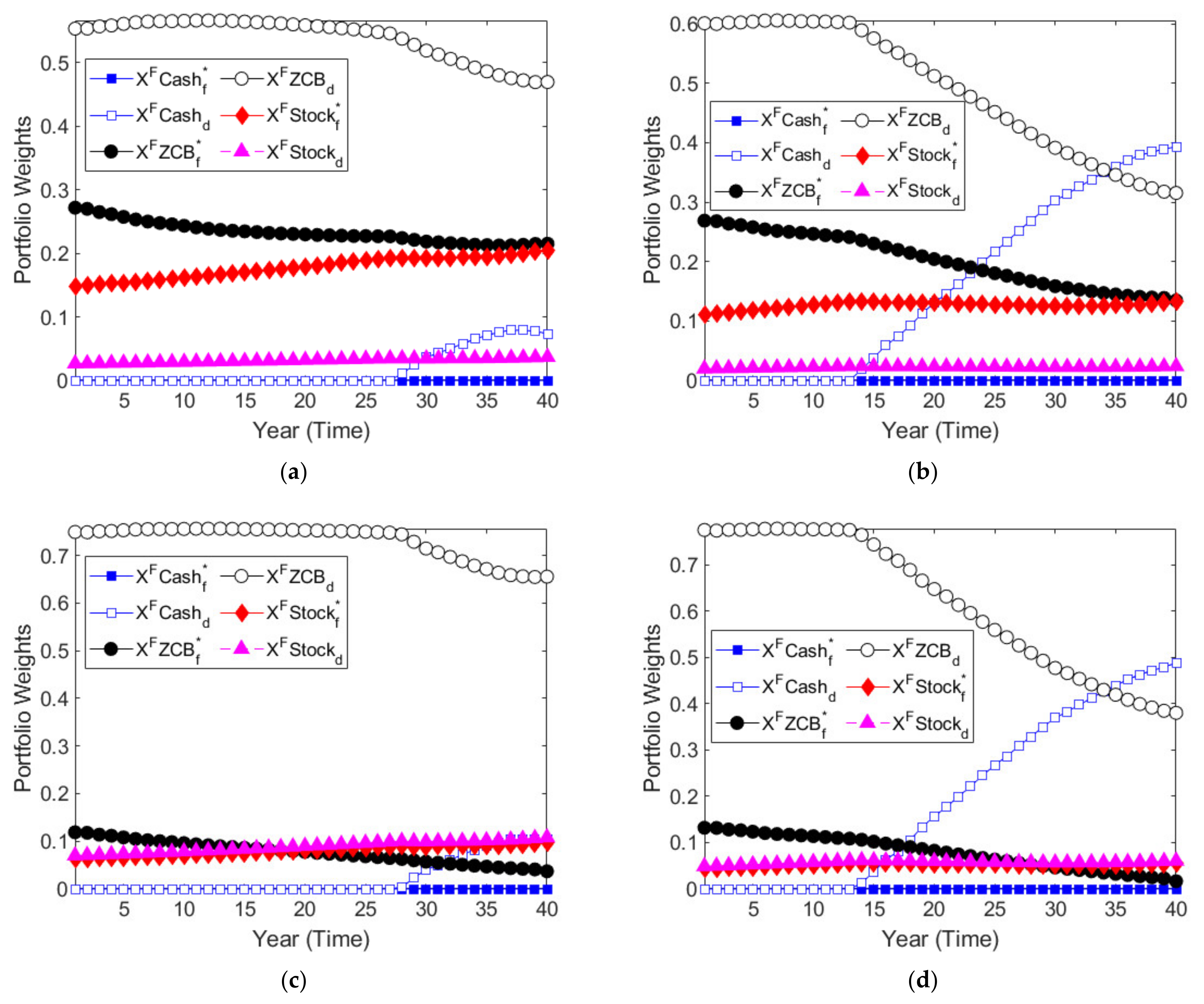
In our study, the most intuitive way to deal with the short sales constraints after dynamic optimization programming is to reset the zero weights in the short positions and then rescale the portfolio’s allocations in proportion to ensure it has invested 100% of the fund. Figure 3 then shows just the optimal proportions of the pension fund’s allocations, with no short sales and no excessive investment leverage, which means its allocative weights all range between 0 and 1.

The subfigures in Figure 3 have similar allocative patterns to Figure 1 and Figure 2, except that the fund’s allocations are shown to shrink when the short sales and leverage constraints are enforced. The short sales constraint restricts financing from both the domestic and foreign cash assets and thus limits the leverage investments in risky assets such as stocks and bonds in both domestic and foreign terms. In general, the domestic bond still occupies the predominant weight so that the pension fund can satisfy its minimum guarantee as its top priority.

Nonetheless, when the fund becomes much more risk-averse, as shown in the subfigures (b) and (d) relative to those in (a) and (c), the domestic bond and domestic cash positions gradually replace each other. The ultimate inclination to hold more domestic cash relative to domestic bonds reflects the fund’s conservative favorite position in increasingly holding the riskless asset in the final accumulation phase for fulfilling the upcoming payment obligation in annuities. Additionally, when the exchange rate is very volatile, as shown in the subfigures (c) and (d) relative to those in (a) and (b), investment weights in foreign risky assets such as foreign bonds and foreign stocks are obviously decreased in response to the severe exchange rate uncertainty.

Overall, the allocative patterns of the subfigures in Figure 3 are alike in comparison with those of Figures 7, 10, and 11 in the aforementioned study [27], which generally compress the leverage positions and limit zero weights in the short positions relative to a comparable scenario with no short sales constraints.

5. Conclusions

Fluctuations in foreign exchange rates have become increasingly important as pension funds consciously shift from local to global investments. To the best of our knowledge, our two-country model is the first model that effectively implements the cross-currency HJM framework in optimizing pension fund management with foreign investment. Our study contributes to building explicitly theoretical criteria with regard to international asset allocation for a self-contained DC pension plan in a stochastic environment that fully contains security risks, interest rate risks, exchange rate risks, and minimum guarantees. In contrast to the conventional framework of equilibrium interest rates adopted in programming- and dynamics-based portfolio research, the cross-currency HJM model can help to demonstrate the dynamics of assets’ price paths and solve the aforementioned stochastic dynamic programming problem of a DC pension plan. The dynamic programming submodel under the cross-currency HJM model then enables the concise representation of assets’ stochastic paths for both domestic and foreign economies.

Since the proposed solution can determine the relationships between stochastic dynamics in exchange rates and domestic and foreign interest rates, this provides a solution for programming optimization. Our study then further contributes to applying numerical analyses based on extracted estimates from real-world market data rather than using presumed estimates. The numerical analyses involved different scenarios and considered various degrees of risk aversion and the risk volatility of exchange rates. The results specifically reveal the different preferences for asset allocation (e.g., foreign versus domestic assets and risky versus riskless assets) during the pension fund’s accumulation phase. In a case involving foreign currency depreciation during our sample period, the optimal allocation strategy for a DC pension plan generally involves first holding bonds and stocks but then shorting cash assets in both foreign and domestic economies in the preliminary accumulation phase; the long positions are then reduced (and vice versa for cash assets). When allocative wisdom is applied, foreign cash is generally chosen as the main short-sale asset. It may be replaced by domestic cash if the foreign exchange market is volatile.

A limitation of this study is that, in practice, some pension funds may be regulated and unable to short-sell or leverage. Therefore, the present work could be extended. One possible extension is to include the short-selling and leverage constraints for developing other applicable allocation criteria of a DC pension plan under exchange rate risks and regulatory restrictions. Moreover, our two-country model could be extended to a multicountry model as the exposed exchange rate risks for a global fund can be multidimensional in practice. These are left for future research on the challenge of solving a comprehensive stochastic dynamic programming problem for a DC pension plan in a multinational investment environment.