Uniform Asymptotics of Solutions of Second-Order Differential Equations with Meromorphic Coefficients in a Neighborhood of Singular Points and Their Applications

Abstract

In this paper, we consider the problem of obtaining the asymptotics of solutions of differential operators in a neighborhood of an irregular singular point. More precisely, we construct uniform asymptotics for solutions of linear differential equations with second-order meromorphic coefficients in a neighborhood of a singular point and apply the results obtained to the equations of mathematical physics. The main results related to the construction of uniform asymptotics are obtained using resurgent analysis methods applied to differential equations with irregular singularities. These results allow us to construct asymptotics for any second-order equations with meromorphic coefficients—that is, with an arbitrary order of degeneracy. This also allows one to determine the type of a singular point and highlight the cases where the point is non-singular or regular.

1. Introduction

One of the fundamental sections of the theory of differential equations is the problem of constructing asymptotics for solutions of second-order equations in neighborhoods of regular and irregular singular points. The problem of constructing asymptotics for solutions of general boundary value problems for elliptic and parabolic equations in domains whose boundary contains a finite number of conic points is considered in Kondratiev’s papers [1,2], where solutions are considered in special spaces of functions that have derivatives summable with some weight. These spaces capture well the main feature of the solutions of such problems, in the sense that the solution is smooth everywhere except at conical points, and when approaching a conical point, the derivatives have power singularities. Moreover, these papers also show that for any linear differential equation with a regular singular point, the asymptotics of the solutions are conormal. The results obtained there make it possible to construct asymptotics for solutions of partial differential equations in a neighborhood of a regular singularity, as well as to obtain asymptotics for solutions of the Laplace equation defined on a manifold with a conical singularity.

One of the first papers that laid the foundation for a systematic study of problems on the construction of asymptotics of solutions in a neighborhood of infinity was Tomé’s paper [3], where for a particular case it was shown that the asymptotics of the solution of the problem under consideration can be represented as a formally divergent power series.

In a general setting, the problem of constructing asymptotics of solutions in a neighborhood of an irregular singular point for differential equations was formulated by Poincaré in [4,5], and also, a particular case of this problem was considered when the irregular singular point is infinity. In these papers, it was proved that the obtained formal divergent series are asymptotic series, and the idea was formulated that an integral transformation can be used to sum the obtained asymptotic series; in a particular case, it could be the Laplace transform. Using this integral transformation, an attempt was made to construct uniform asymptotics of this problem. However, the Laplace integral transform is applicable only in some particular cases. Therefore, the problem of constructing uniform asymptotics for differential equations with holomorphic coefficients in a neighborhood of infinity, which was formulated by Poincaré, has not yet been solved in the general case.

In [6], for second-order equations, the problem of constructing asymptotics of solutions in a neighborhood of infinity was considered—more precisely, the construction of asymptotics of solutions in the case of an irregular singular point, when the order of degeneracy is 2. In this case, the plane is divided into sectors, in each of which the asymptotics is constructed.

In [7], uniform asymptotics of solutions for the Helmholtz equation with constant coefficients were constructed in the two-dimensional case, which is a special case of the example considered in this paper.

In [8], uniform asymptotics are constructed for a wide class of differential equations, but there are sixth and higher order equations for which the asymptotics of solutions in the neighborhood of infinity have not yet been constructed.

In this article, we consider the problem of obtaining the asymptotics of solutions of second-order differential equations in a neighborhood of an irregular singular point. Namely, we first construct the asymptotics of solutions for arbitrary second-order ordinary differential equations with meromorphic coefficients, that is, with an arbitrary irregular singularity, and then we generalize this result to different types of second-order partial differential equations. Next, we show that our results can be used to construct asymptotics for the solution of the Laplace equation on a manifold with a beak-like singularity (see, for example, [9]).

The figures depict a cone and a beak (Figure 1 and Figure 2).

Figure 1. Cone.

Figure 2. Beak.

In [10], it is proved that any linear ordinary differential equation with holomorphic coefficients of order n can be represented as

$$\left({\left(-r^k\frac{d}{dr}\right)}^n+{\displaystyle \sum _{i=0}^{n-1}}{a}_i^0\left(r\right){\left(-r^k\frac{d}{dr}\right)}^i\right)u=0,$$

(1)

in which the formula for calculating the minimum non-negative $k\in Z$ is also obtained, and $a_i^0\left(r\right)={\sum }_{j=0}^{\infty }{a}_i^j{r}^j$ are holomorphic functions.

The operator symbol in (1) is the function

$$H(r,p)=p^n+{\displaystyle \sum _{i=0}^{n-1}}{a}_i^0\left(r\right)p^i,$$

and the main symbol of the differential operator is the function

$$H_0\left(p\right)=H(0,p)=p^n+{\displaystyle \sum _{i=0}^{n-1}}{a}_i^0\left(0\right)p^i.$$

A special case, when the roots of the main symbol are simple, was considered in [11] and then in the classical literature (see, for example, [6,12,13]), in which asymptotic expansions of solutions of some differential equations are constructed, and they are presented as products of the corresponding exponents by divergent power series:

$$u=e^{{\alpha }_1/r}{r}^{{\sigma }_1}{\displaystyle \sum _{k=0}^{\infty }}{a}_1^k{r}^k+e^{{\alpha }_2/r}{r}^{{\sigma }_2}{\displaystyle \sum _{k=0}^{\infty }}{a}_2^k{r}^k\dots +e^{{\alpha }_n/r}{r}^{{\sigma }_n}{\displaystyle \sum _{k=0}^{\infty }}{a}_n^k{r}^k,$$

(2)

where ${\alpha }_i,i=1,\cdots ,n$ are the roots of the polynomial $H_0\left(p\right)$, and $s_j$ and $a_i^k$ are some complex numbers.

The question of interpreting the obtained divergent series included in the expression defining the semi-classical asymptotics was left open; that is, there is no method for summing these divergent series. This question was solved in [14,15], where uniform asymptotics were constructed for this case.

If the asymptotic expansion (2) has at least two terms corresponding to the values ${\alpha }_1$ and ${\alpha }_2$ with different real parts (for definiteness, we assume that $Re{\alpha }_1>Re{\alpha }_2$), there is a significant difficulty in interpreting the obtained expansion. The point is that all terms of the second element of the semiclassical asymptotics (2) for $r\to 0,r>0$ are infinitesimal with respect to any term of the first element; that is, the first element is dominant and the second recessive. However, when the point r moves along the complex plane, the roles of the dominant and recessive components of the expansion can change places. In other words, the plane is conditionally divided into sectors in which one of the components is dominant and the other is recessive, and when moving from one sector to another, there is a change in leadership (the recessive becomes the main one and vice versa). However, in the neighborhood of the boundaries of these sectors, several components are of equal order, and none of them can be neglected. This phenomenon (the Stokes phenomenon) arises, for example, when considering Euler’s example (see [7]). This leads to the fact that the study of asymptotic expansions of solutions to the Equation (1) requires the introduction of a regular method of summation of divergent series to construct uniform asymptotics of solutions with respect to the variable r.

The summation method of similar asymptotic series based on the Laplace–Borel transform and the concept of a resurgent function was first introduced by J. Ecal [16]. This method was then used in the papers of B.-V. Schulze, B.Yu. Sternin, and V.E. Shatalov to study degenerate equations obtained by considering elliptic equations on manifolds with isolated singularities of the beak type, as well as to construct asymptotics for equations with a small parameter. In some cases, in weighted Sobolev spaces, for equations with a parameter and equations with degeneracy of the beak type, they managed to construct asymptotics for solutions (see [17,18,19]).

The main idea of resurgent analysis is that the Laplace–Borel transformations of the asymptotic series included in the quasi-classical asymptotics are power series in the dual variable p, converging in a neighborhood of the points ${\alpha }_j$. The inverse Borel transform then gives a regular way of summing these series. However, in this case, it is necessary to prove the infinite extension of the Laplace–Borel images of the solutions. For equations with irregular singular points, the proof of infinite extension was obtained in the papers of V. Shatalov and M. Korovina [9,14,15]. The results obtained in these articles make it possible to apply the methods of resurgent analysis to the construction of asymptotics for solutions of linear differential equations with holomorphic coefficients.

Second-order differential equations with singular points are used in various areas of mechanics. For example, the Laplace operator written in spherical coordinates has a singular point at zero [9]. In addition, a second-order equation of this type is used to solve the plane problem of finding the stress–strain state of a body of rectangular cross section with a cylindrical cavity in the motion of an ideal incompressible fluid [20]. In this case, equations with an irregular singular point arise. Another example of a second-order equation with a singular point, the DPE (Density Profile Equation), was studied by F. dell’Isola et al. [21,22].

Note also the papers [23,24,25,26,27], in which conormal asymptotics for solutions of elliptic operators are obtained. The resulting asymptotic representations in weighted Sobolev spaces were used in the study of basic boundary value problems for elliptic equations and systems.

In order to proceed to the construction of asymptotics for solutions of equations of mathematical physics, we first solve the problem of constructing uniform asymptotics in the neighborhood of an irregular singularity for ordinary differential equations; that is, we solve the Poincaré problem for second-order differential equations.

In Section 2, definitions and auxiliary statements are given.

In Section 3, the main result (Theorem 3) is formulated and proved, in which the asymptotics of solutions of ODEs with meromorphic coefficients are constructed in a neighborhood of some singular point, finite or infinite.

In Section 4, partial differential equations are considered and, in various examples, asymptotics of solutions for hyperbolic, parabolic, and elliptic equations are constructed. At the end of this section, examples are considered for the Helmholtz equation, as well as for the Laplace equation on a manifold with isolated singular points.

2. Definitions and Auxiliary Statements

Denote by $S_{R,\epsilon }$ the sector $S_{R,\epsilon }=\left\{r\right|-\epsilon <argr<\epsilon ,\left|r\right|<R\}$.

Definition 1.

A function f is analytical on $S_{R,\epsilon }$ and is of an exponential growth no more than k if there are non-negative constants C and α such that in the sector $S_{R,\epsilon }$ the following inequality is valid:

$$\left|f\right|<C{e}^{a\frac{1}{{\left|r\right|}^k}}.$$

Let us denote by $E_k\left(S_{R,\epsilon }\right)$ the space of functions of k-exponential growth. If $\epsilon$ can be chosen by any of $0<\epsilon \le 2\pi$, then we denote this space as $E_k\left(S_R\right)$; $E_k(S_R,L_2\left(S^1\right))$ is the space of functions of exponential growth as $r\to 0$ with values from $L_2\left(S^1\right)$.

Definition 2.

The k Laplace–Borel transform of the function $f\left(r\right)\in E_k\left(S_{R,\epsilon }\right)$ is the mapping $B_k:E_k\left(S_{R,\epsilon }\right)⟶E\left({\tilde{\mathsf{\Omega }}}_{R,\epsilon }\right)/E\left(C\right)$:

$$B_{k}f={\displaystyle \underset{0}{\overset{r_0}{\int }}}{e}^{-p/r^k}f\left(r\right)\frac{dr}{r^{k+1}},$$

where $r_0$ denotes an arbitrary point of the sector.

The inverse k Laplace–Borel transform is defined by the formula:

$$B_k^{-1}\tilde{f}=\frac{k}{2\pi i}\underset{\tilde{\gamma }}{\int }{e}^{p/r^k}\tilde{f}\left(p\right)dp.$$

The contour $\tilde{\gamma }$ is shown in Figure 3.

Figure 3. Contour $\tilde{\gamma }$ and domain ${\tilde{\mathsf{\Omega }}}_{R,\epsilon }$.

Note that for the k Laplace–Borel transform, the following formulas are true:

$$B_k\circ \left(-\frac{1}{k}{r}^{k+1}\frac{\partial }{\partial r}\right)f\left(r\right)=p{B}_{k}f,\frac{\partial }{\partial p}\circ B_{k}f=-B_k\left(\frac{1}{r^k}f\left(r\right)\right).$$

Definition 3.

The function $\tilde{f}$ is called infinitely extendable if for any number R there is a discrete set of points $Z_R$ in C such that the function $\tilde{f}$ is analytically extended from the initial domain of definition along any path with a length smaller than R, which does not pass through $Z_R$.

Definition 4.

The element f of the space $E_k\left(S_{R,\epsilon }\right)$ is called the k-resurgent function if its k Laplace–Borel transform $\tilde{f}=B_{k}f$ is infinitely extendable.

Theorem 1.

Let f be a resurgent function. Then, the solution of the equation

$$H\left(r,-r^k\frac{d}{dr}\right)u=f$$

is a resurgent function in the space $E_k\left(S_R\right)$.

Theorem 2.

If the polynomial $H_0\left(p\right)$ has simple roots at the points $p_1,\cdots ,p_m$, then in the space $E\left(S_R\right)$, the asymptotic expansion of the solution of the homogeneous equation

$$H\left(r,-r^2\frac{d}{dr}\right)u=0$$

has the form

$$u\left(r\right)\approx {\displaystyle \sum _{j=1}^m}exp\left(\frac{p_j}{r}\right)r^{{\sigma }_j}{\displaystyle \sum _{i=0}^{\infty }}{b}_i^j{r}^i,$$

(3)

where the sum is taken over the union of all the roots of the polynomial $H_0\left(p\right)$; $b_i^j,{\sigma }_j,j=1,\cdots ,m$ are some numbers.

For equations with degeneracy of ($k+1$)-order, where $k\in N$, i.e., for an equation of the form

$$H\left(r,-\frac{1}{k}{r}^{k+1}\frac{d}{dr}\right)u=0:$$

(i) 

In the case when the roots of the main symbol are simple, the asymptotics have the form

$$u\left(r\right)\approx {\displaystyle \sum _{j=1}^m}exp\left(\frac{p_j}{r^k}+{\displaystyle \sum _{i=1}^{k-1}}\frac{{\alpha }_{k-i}^1}{r^{k-i}}\right)r^{{\sigma }_j}{\displaystyle \sum _{i=0}^{\infty }}{b}_i^j{r}^i;$$

(4)

(ii) 

In the case when $k+1=\frac{m}{n}$, $m\in N,k\in N,m>k$, the asymptotics of the solution have the form

$$u\approx \sum _{j}exp\left(\frac{p_j}{r^{\frac{m}{k}-1}}+{\displaystyle \sum _{i=1}^{m-k-1}}\frac{{\alpha }_{m-k-i}^1}{r^{\frac{m-i}{k}-1}}\right)r^{{\sigma }_j}{\displaystyle \sum _{i=0}^{\infty }}{b}_i^j{r}^i.$$

(5)

The proof of these theorems can be found in [14,15].

3. Main Results

Consider the equation

$${\left(\frac{d}{dr}\right)}^{2}u+a_1\left(r\right)\left(\frac{d}{dr}\right)u+a_0\left(r\right)u=0,$$

(6)

where the functions $a_1\left(r\right),a_0\left(r\right)$ expand into Laurent series

$$a_1\left(r\right)=r^{-m}{\displaystyle \sum _{j=0}^{\infty }}{b}_j{r}^j,a_0\left(r\right)=r^{-k}{\displaystyle \sum _{j=0}^{\infty }}{c}_j{r}^j;$$

we choose the numbers $m,k\in Z$ so that the condition $b_0\ne 0,c_0\ne 0$ is satisfied. The point $r=0$ is, in general, a singular point of the Equation (6).

Let us construct asymptotics for the solution of the Equation (6) in a neighborhood of zero. Let us rewrite Equation (6) as

$${\left(\frac{d}{dr}\right)}^{2}u+r^{-m}{\displaystyle \sum _{j=0}^{\infty }}{b}_j{r}^j\left(\frac{d}{dr}\right)u+r^{-k}{\displaystyle \sum _{j=0}^{\infty }}{c}_j{r}^{j}u=0.$$

(7)

Since the following equality holds

$$\begin{array}{c}{r}^k{\left(\frac{d}{dr}\right)}^2={\left(r^{\frac{k}{2}}\frac{d}{dr}\right)}^2-\frac{k}{2}{r}^{\frac{k}{2}-1}\left(r^{\frac{k}{2}}\frac{d}{dr}\right),\hfill \end{array}$$

Equation (7) can be rewritten in the form

$${\left(r^{\frac{k}{2}}\frac{d}{dr}\right)}^{2}u-\frac{k}{2}{r}^{\frac{k}{2}-1}\left(r^{\frac{k}{2}}\frac{d}{dr}\right)u+r^{\frac{k}{2}-m}{\displaystyle \sum _{j=0}^{\infty }}{b}_j{r}^j\left(r^{\frac{k}{2}}\frac{d}{dr}\right)u+{\displaystyle \sum _{j=0}^{\infty }}{c}_j{r}^{j}u=0.$$

(8)

Theorem 3.

All asymptotics of the solution of the Equation (7) in spaces of exponential growth functions can be represented as

1. 

Let $k>2m$. If $k>2$, then

(i) 

For $k=2n+1,n=1,2,\cdots$ the asymptotics of the solution of the Equation (7) has the form

$$\begin{array}{c}u\left(r\right)\approx exp\left(\frac{p_1}{r^{n-\frac{1}{2}}}+{\displaystyle \sum _{i=1}^{2n-2}}\frac{{\alpha }_i^1}{r^{n-\frac{i}{2}-\frac{1}{2}}}\right)r^{{\sigma }_1}{\displaystyle \sum _{i=0}^{\infty }}{b}_i^1{r}^{\frac{i}{2}}+exp\left(\frac{p_2}{r^{n-\frac{1}{2}}}+{\displaystyle \sum _{i=1}^{2n-2}}\frac{{\alpha }_i^2}{r^{n-\frac{i}{2}-1}}\right)r^{{\sigma }_2}{\displaystyle \sum _{i=0}^{\infty }}{b}_i^2{r}^{\frac{i}{2}},\hfill \\ u\left(r\right)\in E_{n-\frac{1}{2}}\left(S_R\right);\hfill \end{array}$$

(9)

(ii) 

For $k=2n,n=2,3,\cdots$

$$\begin{array}{c}u\left(r\right)\approx exp\left(\frac{p_1}{r^{n-1}}+{\displaystyle \sum _{i=1}^{n-2}}\frac{{\alpha }_i^1}{r^{n-1-i}}\right)r^{{\sigma }_1}{\displaystyle \sum _{i=0}^{\infty }}{b}_i^1{r}^i+exp\left(\frac{p_2}{r^{n-1}}+{\displaystyle \sum _{i=1}^{n-2}}\frac{{\alpha }_i^2}{r^{n-i-1}}\right)r^{{\sigma }_2}{\displaystyle \sum _{i=0}^{\infty }}{b}_i^2{r}^i,\hfill \\ u\left(r\right)\in E_{n-1}\left(S_R\right),\hfill \end{array}$$

(10)

where $p_1$, $p_2$ are the roots of the polynomial

$$H_0\left(p\right)=p^2+{\left(\frac{1}{\frac{k}{2}-1}\right)}^2{c}_0.$$

(iii) 

For $k=2$ or $k=1,m=0,-1,\cdots$, the asymptotics of the solution are conormal.

(iv) 

For $k\le 0$, the solution is holomorphic.

2. 

Let $k<2m$. If $m>1$, then the asymptotics of the solution have the form

$$\begin{array}{c}u\approx exp\left({\displaystyle \sum _{i=2}^{m-1}}\frac{{\alpha }_i^1}{r^{m-i}}\right){\displaystyle \sum _{i=0}^{\infty }}{b}_i^1{r}^i+r^{\sigma }exp\left(-\frac{p_2}{r^{m-1}}+{\displaystyle \sum _{i=2}^{m-1}}\frac{{\alpha }_i^2}{r^{m-i}}\right){\displaystyle \sum _{i=0}^{\infty }}{A}_i^2{r}^i,\hfill \\ u\left(r\right)\in E_{m-1}\left(S_R\right);\hfill \end{array}$$

here $p_2=b_0/(m-1)$.

(i) 

If $m=1$, then the asymptotics is conormal.

(ii) 

If $m<1$, then the solution is holomorphic.

3. 

Let $k=2m$.

(i) 

If $m=1$, then the asymptotics of the solution are conormal.

(ii) 

If $m>1$, and if the roots are $p_1$, $p_2$ of the polynomial

$$H_0\left(p\right)=p^2-\frac{b_0}{m-1}p+c_0{\left(\frac{1}{m-1}\right)}^2$$

do not coincide, then the asymptotics have the form

$$u\left(r\right)\approx r^{{\sigma }_1}exp\left(-\frac{p_1}{r^{m-1}}+\sum _{i=2}^{m-1}\frac{{\alpha }_i^1}{r^{m-i}}\right)\sum _{i=0}^{\infty }{b}_i^1{r}^i+r^{{\sigma }_2}exp\left(-\frac{p_2}{r^{m-1}}+\sum _{i=‘2}^{m-1}\frac{{\alpha }_i^2}{r^{m-i}}\right)\sum _{i=0}^{\infty }{b}_i^2{r}^i.$$

(iii) 

If $p_1=p_2=\alpha$, then the problem reduces to the previous cases.

Here, by ${\sum }_{i=0}^{\infty }{b}_i^j{r}^i,j=1,2$ denotes the corresponding asymptotic series, while ${\alpha }_i^j,{\sigma }_j,j=1,2,\cdots ,$$i=1,\cdots ,n-2$ are some constants.

Proof. 

To prove the theorem, we consider three cases: (i) $k>2m$; (ii) $k<2m$; (iii) $k=2m$.

Case (i): $k>2m$. Under the condition $k>2m,k>2$, the Equation (8) has an irregular singularity. Let us rewrite the equation as

$$\begin{array}{c}{\left(-\frac{1}{\frac{k}{2}-1}{r}^{\frac{k}{2}}\frac{d}{dr}\right)}^{2}u-\frac{1}{\frac{k}{2}-1}{r}^{\frac{k}{2}-m}{\displaystyle \sum _{j=0}^{\infty }}{b}_j{r}^j\left(-\frac{1}{\frac{k}{2}-1}{r}^{\frac{k}{2}}\frac{d}{dr}\right)u+\hfill \\ +{\left(\frac{1}{\frac{k}{2}-1}\right)}^2{\displaystyle \sum _{j=0}^{\infty }}{c}_j{r}^{j}u+\frac{k}{2\left(\frac{k}{2}-1\right)}{r}^{\frac{k}{2}-1}\left(-\frac{1}{\frac{k}{2}-1}{r}^{\frac{k}{2}}\frac{d}{dr}\right)u=0.\hfill \end{array}$$

(11)

The main symbol of the Equation (11) has the form

$$H_0\left(p\right)=p^2+{\left(\frac{1}{\frac{k}{2}-1}\right)}^2{c}_0$$

Denote by $p_1,p_2$ the roots of this polynomial. Theorem 1 implies that the asymptotics of the solution (11) have the form

$$u\approx exp{\left(\frac{p_1}{r^{\frac{k}{2}-1}}+\sum _{i=1}^{k-3}\frac{{\alpha }_{k-2-i}^1}{r^{\frac{k-i}{2}-1}}\right)}^{}{r}^{{\sigma }_1}\sum _{i=0}^{\infty }{b}_i^1{r}^{\frac{i}{2}}+exp{\left(\frac{p_2}{r^{\frac{k}{2}-1}}+\sum _{i=1}^{k-3}\frac{{\alpha }_{k-2-i}^2}{r^{\frac{k-i}{2}-1}}\right)}^{}{r}^{{\sigma }_2}\sum _{i=0}^{\infty }{b}_i^2{r}^{\frac{i}{2}}$$

Let us separately consider the cases $k=2$ and $k=1$ with $m=0,-1,\cdots$. In the case of $k=2$, Equation (8) becomes

$${\left(r\frac{d}{dr}\right)}^{2}u-\left(r\frac{d}{dr}\right)u+r^{1-m}\sum _{j=0}^{\infty }{b}_j{r}^j\left(r\frac{d}{dr}\right)u+\sum _{j=0}^{\infty }{c}_j{r}^{j}u=0.$$

Let $k=1$ and $m=0,-1,\cdots$. Then, Equation (8) takes the form

$${\left(r\frac{d}{dr}\right)}^{2}u-\left(r\frac{d}{dr}\right)u+r^{1-m}\sum _{j=0}^{\infty }{b}_j{r}^j\left(r\frac{d}{dr}\right)u+r\sum _{j=0}^{\infty }{c}_j{r}^{j}u=0.$$

In these two cases, the asymptotics of the solution are conormal.

Thus, in the case for $k>2$, the asymptotics of the solution of the Equation (8) are asymptotics of the non-Fuchsian type; for $0<k\le 2$, the asymptotics are conormal.

Obviously, for $k\le 0$, the solution is a holomorphic function.

Case (ii): $k<2m$. Multiplying Equation (6) by $r^{2m}$ and making elementary transformations, we get

$${\left(r^m\frac{d}{dr}\right)}^{2}u-m{r}^{m-1}\left(r^m\frac{d}{dr}\right)u+\sum _{j=0}^{\infty }{b}_j{r}^j\left(r^m\frac{d}{dr}\right)u+r^{2m-k}\sum _{j=0}^{\infty }{c}_j{r}^{j}u=0.$$

(12)

Let $m>1$. Let us rewrite Equation (12) as

$$\begin{array}{c}{\left(-\frac{1}{m-1}{r}^m\frac{d}{dr}\right)}^{2}u+\frac{m}{m-1}{r}^{m-1}\left(-\frac{1}{m-1}{r}^m\frac{d}{dr}\right)u-\frac{b_0}{m-1}\left(-\frac{1}{m-1}{r}^m\frac{d}{dr}\right)u-\hfill \\ -\left(\frac{1}{m-1}\right){\displaystyle \sum _{j=1}^{\infty }}{b}_j{r}^j\left(-\frac{1}{m-1}{r}^m\frac{d}{dr}\right)u+r^{2m-k}{\left(-\frac{1}{m-1}\right)}^2{\displaystyle \sum _{j=0}^{\infty }}{c}_j{r}^{j}u=0.\hfill \end{array}$$

(13)

The main symbol of the operator from (13) is

$$H_0\left(p\right)=p^2-\frac{b_0}{m-1}p=p\left(p-\frac{b_0}{m-1}\right)$$

with two simple roots $p_1=0,p_2=\frac{b_0}{m-1}$.

From Theorem 2, it follows that the asymptotics of the solution to Equation (13) have the form

$$exp\left(\sum _{i=2}^{m-1}\frac{{\alpha }_i^0}{r^{m-i}}\right)\sum _{i=0}^{\infty }{A}_i^1{r}^i+r^{\sigma }exp\left(-\frac{b}{r^{m-1}}+\sum _{i=2}^{m-1}\frac{{\alpha }_i^1}{r^{m-i}}\right)\sum _{i=0}^{\infty }{A}_i^2{r}^i$$

If $m=1$, then Equation (12) takes the form

$${\left(r\frac{d}{dr}\right)}^{2}u-\left(r\frac{d}{dr}\right)u+\sum _{j=0}^{\infty }{b}_j{r}^j\left(r\frac{d}{dr}\right)u+r^{2-k}\sum _{j=0}^{\infty }{c}_j{r}^{j}u=0,$$

that is, the asymptotics of the solution are conormal.

Thus, for $k<2m$, we have obtained that for $1<m$ the asymptotics will be non-Fuchsian; for $m=1$, the asymptotics will be conormal.

As above, it is easy to see that for $m\le 0$, the solution is a holomorphic function.

Case (iii): $k=2m$. Let $m=1$. Then, Equation (8) takes the form

$${\left(r\frac{d}{dr}\right)}^{2}u-\left(r\frac{d}{dr}\right)u+\sum _{j=0}^{\infty }{b}_j{r}^j\left(r\frac{d}{dr}\right)u+r^{2-k}\sum _{j=0}^{\infty }{c}_j{r}^{j}u=0.$$

Therefore, the asymptotics of the solution of this equation are conormal.

Let $m>1$. Then, Equation (8) is transformed to the form

$$\begin{array}{c}{\left(-\frac{1}{m-1}{r}^m\frac{d}{dr}\right)}^{2}u-\frac{b_0}{m-1}\left(-\frac{1}{m-1}{r}^m\frac{d}{dr}\right)u+c_0{\left(\frac{1}{m-1}\right)}^{2}u-\hfill \\ -\left(\frac{1}{m-1}\right){\displaystyle \sum _{j=1}^{\infty }}{b}_j{r}^j\left(-\frac{1}{m-1}{r}^m\frac{d}{dr}\right)u+{\left(\frac{1}{m-1}\right)}^2{\displaystyle \sum _{j=1}^{\infty }}{c}_j{r}^{j}u-\frac{m}{m-1}{r}^{m-1}\left(-\frac{1}{m-1}{r}^m\frac{d}{dr}\right)u=0.\hfill \end{array}$$

The main symbol of the operator from the last equation has the form

$$H_0\left(p\right)=p^2-\frac{b_0}{m-1}p+c_0{\left(\frac{1}{m-1}\right)}^2.$$

Denote by $p_1,p_2$ two roots of this polynomial.

If $p_1\ne p_2$, then the roots are simple, and it follows from Theorem 2 that the asymptotics of the solution have the form

$$r^{{\sigma }_1}exp\left(-\frac{p_1}{r^{m-1}}+\sum _{i=2}^{m-1}\frac{{\alpha }_i^0}{r^{m-i}}\right)\sum _{i=0}^{\infty }{A}_i^1{r}^i+r^{{\sigma }_2}exp\left(-\frac{p_2}{r^{m-1}}+\sum _{i=2}^{m-1}\frac{{\alpha }_i^1}{r^{m-i}}\right)\sum _{i=0}^{\infty }{A}_i^2{r}^i.$$

If $p_1=p_2=\alpha$, then by changing the variable $u=e^{-\frac{\alpha }{r^{m-1}}}{u}_1$, from (7), we obtain an equation of the form

$${\left(\frac{d}{dr}\right)}^2{u}_1+r^{-m+1}\sum _{j=0}^{\infty }{b}_j^{\prime }{r}^j\left(\frac{d}{dr}\right)u_1+r^{2m+1}\sum _{j=0}^{\infty }{c}_j^{\prime }{r}^j{u}_1=0,$$

where $b_j^{\prime }$, $c_j^{\prime }$ are the corresponding constants.

To construct the asymptotics of this equation, it is necessary to apply the method described above.

If $m<1$, then the solution is holomophic. □

4. Examples

In this section, we illustrate the application of Theorems 2 and 3 both to second-order differential equations and to the basic operators of mathematical physics.

Let $\mathsf{\Omega }\subset {\mathbb{R}}^n$ be a domain with smooth boundary $\partial \mathsf{\Omega }$. Denote by $Q_{\infty }=\mathsf{\Omega }\times (0<t<\infty )$ the cylinder containing the points $(x,t)\in {\mathbb{R}}^{n+1}$; $\partial Q_{\infty }=\partial \mathsf{\Omega }\times (0\le t<\infty )$ is the lateral surface of the cylinder.

4.1. Construction of Asymptotics for Solutions of Second-Order Equations with Meromorphic Coefficients in a Neighborhood of Infinity

Consider the equation

$${\left(\frac{d}{dt}\right)}^{2}u+a^0\left(t\right)\left(\frac{d}{dt}\right)u+c^0\left(t\right)u=0;$$

(14)

where the functions $a^0\left(t\right),c^0\left(t\right)$ have poles at infinity; that is, in the exterior of the circle $\left|t\right|>R$, the functions $a^0\left(t\right),c^0\left(t\right)$ can be expanded in Laurent series

$$a^0\left(t\right)=t^m\sum _{j=0}^{\infty }\frac{a_j}{t^j},c^0\left(t\right)=t^k\sum _{j=0}^{\infty }\frac{c_j}{t^j}.$$

We choose $m\in Z,k\in Z$ so that $a_0^{}\ne 0,c_0\ne 0$.

Let us construct the asymptotics of the solution of Equation (14) as $t\to \infty$. Let us make the change $t=1/r$.

Since

$$\frac{d}{dt}v\left(t\right)=\frac{dv}{dr}\frac{dr}{dt}=-\frac{1}{t^2}\frac{dv}{dr}=-r^2\frac{dv}{dr},$$

then from Equation (14), we get

$${\left(-r^2\frac{d}{dr}\right)}^{2}v\left(r\right)+a\left(r\right)\left(-r^2\frac{d}{dt}\right)v\left(r\right)+c\left(r\right)v\left(r\right)=0,$$

(15)

where

$$a\left(r\right)=r^{-m}\sum _{j=0}^{\infty }{a}_j^{}{r}^j,c\left(r\right)=r^{-k}\sum _{j=0}^{\infty }{c}_j{r}^j.$$

Taking into account the obvious identity

$$r^4{\left(\frac{d}{dr}\right)}^2={\left(-r^2\frac{d}{dr}\right)}^2-2r^{}\left(r^2\frac{d}{dr}\right),$$

Equation (15) is converted to the form

$$r^4{\left(\frac{d}{dr}\right)}^{2}v\left(r\right)+2r\left(r^2\frac{d}{dr}\right)v\left(r\right)+r^{-m}\sum _{j=0}^{\infty }{a}_j{r}^j\left(-r^2\frac{d}{dt}\right)v\left(r\right)+r^{-k}\sum _{j=0}^{\infty }{c}_j{r}^{j}v\left(r\right)=0,$$

(16)

and making elementary transformations, we get

$${\left(\frac{d}{dr}\right)}^{2}v\left(r\right)+2r^{-1}\left(\frac{d}{dr}\right)v\left(r\right)+r^{-m-2}\sum _{j=0}^{\infty }{a}_j{r}^j\left(\frac{d}{dt}\right)v\left(r\right)+r^{-k-4}\sum _{j=0}^{\infty }{c}_j{r}^{j}v\left(r\right)=0.$$

(17)

Thus, the asymptotics of the solution of the Equation (17) are constructed according to Theorem 3.

4.2. Wave Equation

Consider the wave equation

$${\left(\frac{d}{dt}\right)}^{2}u(x,t)-a^0\left(t\right)\Delta u(x,t)=0,(x,t)\in Q_{\infty }$$

(18)

with the boundary condition

$${\left.\left(\alpha u+\beta \frac{\partial u}{\partial \nu }\right)\right|}_{\partial Q_{\infty }}=0;$$

(19)

here $\alpha \left(x\right)\ge 0,\beta \left(x\right)\ge 0$, $\alpha \left(x\right)\not\equiv 0,\alpha \left(x\right)+\beta \left(x\right)>0$, $\nu =({\nu }_1,\cdots ,{\nu }_n)$ is the outer unit normal vector to $\partial \mathsf{\Omega }$, the function $a^0\left(t\right)\ge 0$ is holomorphic in a neighborhood of infinity or has a pole at infinity; that is, there exists an exterior of the circle $\left|t\right|>R$ such that the function $a^0\left(t\right)$ expands in it in a Laurent series

$$a^0\left(t\right)=t^k\sum _{j=0}^{\infty }\frac{a_j}{t^j},$$

(20)

where $k\in Z$, and k can always be chosen so that the condition $a_0\ne 0$ is fulfilled.

If $k\le 0$, then the series (20) in the neighborhood of infinity is a Taylor series.

Let us construct the asymptotics of the solution of the problem (18) and (19) as $t\to \infty$, in the space of functions of exponential growth [28].

Using the method of separation of variables, we look for a solution in the form $u(x,t)=Y\left(x\right)v\left(t\right)$, and we obtain a system of equations

$$\Delta Y\left(x\right)+\lambda Y\left(x\right)=0,$$

(21)

$${\left(\frac{d}{dt}\right)}^{2}v\left(t\right)+a^0\left(t\right)\lambda v\left(t\right)=0$$

(22)

and the boundary condition

$$\begin{array}{c}{\left.\left(\alpha Y+\beta \frac{\partial Y}{\partial \nu }\right)\right|}_{\partial \mathsf{\Omega }}=0.\hfill \end{array}$$

(23)

Denote by ${\lambda }_n$ the eigenvalues of the operator corresponding to the problem (21) and (23), and by $Y_n\left(x\right)$ its eigenfunctions.

Since $\alpha \left(x\right)\ge 0,\alpha \left(x\right)\not\equiv 0$, then $\lambda =0$ is not an eigenvalue of the problem (21) and (23).

Lemma 1.

All asymptotics of solutions of Equation (22), in spaces of functions of exponential growth as $t\to \infty$, have the following form:

1. 

Let $k_1=k+4>2$. Then, for $k=2n_1+1,n_1=-1,0,\cdots$, the asymptotics of the solution of the Equation (22) in the space of functions of exponential growth have the form

$$\begin{array}{c}v\left(t\right)\approx exp\left(p_1{t}^{n_1+\frac{3}{2}}+{\displaystyle \sum _{i=1}^{2n-2}}{\alpha }_i^1{t}^{n_1-\frac{i}{2}+\frac{3}{2}}\right)t^{-{\sigma }_1}{\displaystyle \sum _{i=0}^{\infty }}{b}_i^1{t}^{-\frac{i}{2}}+exp{\left(p_2{t}^{n_1+\frac{3}{2}}+{\displaystyle \sum _{i=1}^{2n-2}}{\alpha }_i^2{t}^{n_1-\frac{i}{2}+\frac{3}{2}}\right)}^{}{t}^{-{\sigma }_2}{\displaystyle \sum _{i=0}^{\infty }}{b}_i^2{t}^{-\frac{i}{2}},\hfill \\ v\left(t\right)\in E_{n_1+\frac{3}{2}}\left(S_R\right);\hfill \end{array}$$

2. 

For $k=2n_1,n_1=0,1,\cdots$, the asymptotics of the solution to the Equation (22) in the space of functions of exponential growth have the form

$$\begin{array}{c}v\left(t\right)\approx exp\left(p_1{t}^{n_1+1}+{\displaystyle \sum _{i=1}^n}{\alpha }_i^1{t}^{n_1+1-i}\right)t^{-{\sigma }_1}{\displaystyle \sum _{i=0}^{\infty }}{b}_i^1{t}^{-i}+exp\left(p_2{t}^{n_1+1}+{\displaystyle \sum _{i=1}^n}{\alpha }_i^2{t}^{n_1+1-i}\right)t^{-{\sigma }_2}{\displaystyle \sum _{i=0}^{\infty }}{b}_i^2{t}^{-i},\hfill \\ v\left(t\right)\in E_{n_1+1}\left(S_R\right),\hfill \end{array}$$

where $p_1$, $p_2$ are the roots of the polynomial

$$H_0\left(p\right)=p^2+{\left(\frac{1}{\frac{k_1}{2}-1}\right)}^2\lambda a_0.$$

Under the condition $k_1=k+4\le 2$, the asymptotics of the solution will be conormal.

Proof. 

Let us proceed to the construction of the asymptotics of the Equation (22) as $t\to \infty$. We make the change $1/r$. Then, Equation (22) takes the form

$${\left(-r^2\frac{d}{dr}\right)}^{2}v\left(r\right)+r^{-k}a\left(r\right)\lambda v\left(r\right)=0.$$

(24)

Since

$$r^4{\left(\frac{d}{dr}\right)}^2+2r\left(r^2\frac{d}{dr}\right)={\left(r^2\frac{d}{dr}\right)}^2,$$

then Equation (24) can be rewritten in the form

$${\left(\frac{d}{dr}\right)}^{2}v\left(r\right)+2r^{-1}\left(\frac{d}{dr}\right)v\left(r\right)+r^{-k-4}a\left(r\right)\lambda v\left(r\right)=0.$$

(25)

where $m=1$, and $k_1=k+4$.

First, consider the case $k_1>2m=2$. If $k_1=k+4$, then the asymptotics of the solution of Equation (25) for odd $k_1=2n+1,n=1,\cdots$ are constructed by Equation (9), and in the case of even $k_1$ by Equation (10).

If we introduce the notation $k=2n_1+1,n_1=-1,0,\cdots$, then $k_1=k+4=2n_1+5=2n+1$. Since the equality $n-\frac{1}{2}=\frac{2n_1+5}{2}-1=n_1+\frac{3}{2}$ holds, then from Equation (9), it follows that

$$\begin{array}{c}u\approx exp\left(\frac{p_1}{r^{n-\frac{1}{2}}}+{\displaystyle \sum _{i=1}^{2n-2}}\frac{{\alpha }_i^1}{r^{n-\frac{i}{2}-\frac{1}{2}}}\right)r^{{\sigma }_1}{\displaystyle \sum _{i=0}^{\infty }}{b}_i^1{r}^{\frac{i}{2}}+exp\left(\frac{p_2}{r^{n-\frac{1}{2}}}+{\displaystyle \sum _{i=1}^{2n-2}}\frac{{\alpha }_i^2}{r^{n-\frac{i}{2}-1}}\right)r^{{\sigma }_2}{\displaystyle \sum _{i=0}^{\infty }}{b}_i^2{r}^{\frac{i}{2}}=\hfill \\ =exp\left(\frac{p_1}{r^{n_1+\frac{3}{2}}}+{\displaystyle \sum _{i=1}^{2n-2}}\frac{{\alpha }_i^1}{r^{n_1-\frac{i}{2}+\frac{3}{2}}}\right)r^{{\sigma }_1}{\displaystyle \sum _{i=0}^{\infty }}{b}_i^1{r}^{\frac{i}{2}}+exp\left(\frac{p_2}{r^{n_1+\frac{3}{2}}}+{\displaystyle \sum _{i=1}^{2n-2}}\frac{{\alpha }_i^2}{r^{n_1-\frac{i}{2}+\frac{3}{2}}}\right)r^{{\sigma }_2}{\displaystyle \sum _{i=0}^{\infty }}{b}_i^2{r}^{\frac{i}{2}}.\hfill \end{array}$$

In the case when $k_1=k+4=2n=2n_1+4$, $n_1=0,1,2\cdots$, and since $n-1=frac2n_1+42-1=n_1+1$, Equation (10) implies

$$\begin{array}{c}u\left(r\right)\approx exp\left(\frac{p_1}{r^{n-1}}+{\displaystyle \sum _{i=1}^{n-2}}\frac{{\alpha }_i^1}{r^{n-1-i}}\right)r^{{\sigma }_1}{\displaystyle \sum _{i=0}^{\infty }}{b}_i^1{r}^i+exp\left(\frac{p_2}{r^{n-1}}+{\displaystyle \sum _{i=1}^{n-2}}\frac{{\alpha }_i^2}{r^{n-i-1}}\right)r^{{\sigma }_2}{\displaystyle \sum _{i=0}^{\infty }}{b}_i^2{r}^i=\hfill \\ =exp\left(\frac{p_1}{r^{n_1+1}}+{\displaystyle \sum _{i=1}^n}\frac{{\alpha }_i^1}{r^{n_1+1-i}}\right)r^{{\sigma }_1}{\displaystyle \sum _{i=0}^{\infty }}{b}_i^1{r}^i+exp\left(\frac{p_2}{r^{n_1+1}}+{\displaystyle \sum _{i=1}^n}\frac{{\alpha }_i^2}{r^{n_1-i+1}}\right)r^{{\sigma }_2}{\displaystyle \sum _{i=0}^{\infty }}{b}_i^2{r}^i,\hfill \end{array}$$

where $p_1$, $p_2$ are the roots of the polynomial

$$H_0\left(p\right)=p^2+\lambda {\left(\frac{1}{\frac{k+4}{2}-1}\right)}^2{a}_0={\left(\frac{2}{2+k}\right)}^2\lambda a_0+p^2.$$

If $k_1\le 2m=2$, then taking into account the fact that $m=1$, it follows from Theorem 3 that the asymptotic of the solution is conormal. □

Now, we can construct a general solution for the problems in (18) and (19). Denote by $v_j\left(t\right)$ the solution of Equation (22) with $\lambda ={\lambda }_j$.

Preposition 1.

All asymptotes of solutions to the problem (18) and (19) in the space of exponentially growing functions in the neighborhood of infinity by t can be represented as a linear combination of functions $u_j(x,t)\in E_{k_j}(S_R,L_2\left(\mathsf{\Omega }\right)),j=0,1,\cdots$

$$u_j(x,t)\approx v_j\left(t\right)Y_{{\lambda }_j}\left(x\right).$$

Remark 1.

Theorem 3 is also applicable to the problem where the Klein–Gordon–Fock equation is considered instead of the wave Equation (18).

4.3. Heat Equation

Consider the heat equation

$$\left(\frac{d}{dt}\right)u(x,t)-a^0\left(t\right)\Delta u\left(x,t\right)=0,(x,t)\in Q_{\infty }$$

(26)

with the boundary condition

$${\left.\left(\alpha u+\beta \frac{\partial u}{\partial \nu }\right)\right|}_{\partial Q_{\infty }}=0;$$

(27)

where $\alpha \left(x\right)\ge 0,\beta \left(x\right)\ge 0$, $\alpha \left(x\right)\not\equiv 0,\alpha \left(x\right)+\beta \left(x\right)>0$, $\nu =({\nu }_1,\cdots ,{\nu }_n)$ is the outer unit normal vector to $\partial \mathsf{\Omega }$, and the function $a^0\left(t\right)\ge 0$ is holomorphic in a neighborhood of infinity or has a pole at infinity; that is, there exists such an exterior of the circle $\left|t\right|>R$ that the function $a^0\left(t\right)$ expands in it in a Laurent series (20), where $k\in Z$, and k can always be chosen so that the condition $a_0\ne 0$ is satisfied. If $k\le 0$, then the series (20) in the neighborhood of infinity is a Taylor series.

Let us construct the asymptotics of the solution of the problem (26) and (27) as $t\to \infty$ in the space of functions of exponential growth.

Using the method of separation of variables, we look for a solution in the form $u(x,t)=Y\left(x\right)v\left(t\right)$, and we obtain a system of equations

$$\Delta Y\left(x\right)+\lambda Y\left(x\right)=0,$$

(28)

$$\left(\frac{d}{dt}\right)v\left(t\right)+a^0\left(t\right)\lambda v\left(t\right)=0$$

(29)

and the boundary condition

$$\begin{array}{c}{\left.\left(\alpha Y+\beta \frac{\partial Y}{\partial \nu }\right)\right|}_{\partial \mathsf{\Omega }}=0.\hfill \end{array}$$

(30)

Denote by ${\lambda }_n$ the eigenvalues of the operator corresponding to problems (28) and (30) and through $Y_n\left(x\right)$ the corresponding eigenfunctions.

Lemma 2.

The asymptotics of the solution of Equation (29) as $t\to \infty$ have the form

$$v\left(t\right)\approx exp\left(p_1{t}^{k+1}+{\displaystyle \sum _{i=0}^k}{\alpha }_{k-i}^1{t}^{k-i}\right)t^{-\sigma }{\displaystyle \sum _{i=0}^{\infty }}{b}_i^1{t}^{-i};$$

here $p_1=-\frac{1}{k+1}\lambda a_0$, ${\alpha }_i^1,\sigma$ are some constants, ${\displaystyle \sum _{i=0}^{\infty }}{b}_i^1{t}^i$ is an asymptotic series.

Proof. 

Let us proceed to the construction of the asymptotics of Equation (29) as $t\to \infty$. We make the change $t=1/r$. Then, Equation (29) can be rewritten as

$$\left(-\frac{1}{k+1}{r}^{2+k}\frac{d}{dr}\right)v\left(r\right)+\frac{1}{k+1}a\left(r\right)\lambda v\left(r\right)=0,$$

(31)

for which the main symbol is $H_0\left(p\right)=p+\frac{1}{k+1}\lambda a_0$. Theorem 2 implies

$$v\left(r\right)\approx exp\left(\frac{p_1}{r^{k+1}}+{\displaystyle \sum _{i=0}^k}\frac{{\alpha }_i^1}{r^{k-i}}\right)r^{\sigma }{\displaystyle \sum _{i=0}^{\infty }}{b}_i^1{r}^i,$$

where $p_1=-\frac{1}{k+1}\lambda a_0$, ${\alpha }_i^1,\sigma$ are some constants, and ${\sum }_{i=0}^{\infty }{b}_i^1{r}^i$ is an asymptotic series.

Further, making the reverse change from r to t, we obtain the assertion of Lemma 2. □

Remark 2.

The solution to the (29) equation is

$$\begin{array}{c}v\left(r\right)=Cexp\lambda \left(\int \frac{a_0}{r^{k+2}}dr+\int {\displaystyle \sum _{i=1}^{k+1}}\frac{{\alpha }_i}{r^{k+2-i}}dr+\int {\displaystyle \sum _{i=k+2}^{\infty }}\frac{{\alpha }_i}{r^{k+2-i}}dr\right)=\hfill \\ =Cexp\left(\lambda \frac{a_0}{r^{k+1}}+{\displaystyle \sum _{i=0}^k}\frac{{\alpha }_i^1}{r^{k-i}}\right)r^{\sigma }g\left(r\right),\hfill \end{array}$$

where $g\left(r\right)$ is a holomorphic function and can be represented as

$$g\left(r\right)=Cexp\lambda \int {\displaystyle \sum _{i=k+2}^{\infty }}\frac{{\alpha }_i}{r^{k+2-i}}dr=Cexp\lambda {\displaystyle \sum _{i=k+2}^{\infty }}\frac{{\alpha }_i}{i-k-1}{r}^{i-k-1}.$$

Consequently, the series ${\displaystyle \sum _{i=0}^{\infty }}{b}_i^1{r}^i$ is convergent.

Denote by $v_j^t\left(t\right)$ the solution of the Equation (29) for $\lambda ={\lambda }_j$.

Preposition 2.

All asymptotes of solutions of problems (26) and (27) as $t\to \infty$, in the space of exponentially growing functions, can be represented as a linear combination of functions $u_j(x,t),$$j=0,1,\cdots$, i.e.,

$$u_j(x,t)\approx v_j^t\left(t\right)Y_{{\lambda }_j}\left(x\right).$$

4.4. Asymptotics of the Solution of the Helmholtz Equation

4.4.1. Asymptotics of the Solution of the Helmholtz Equation at Infinity

We write the Laplace operator in polar coordinates

$$\left(\frac{1}{\rho }\frac{\partial }{\partial \rho }\left(\rho \frac{\partial }{\partial \rho }\right)+\frac{1}{{\rho }^2}\frac{{\partial }^2}{\partial {\phi }^2}\right)u+\lambda u=0.$$

(32)

Obviously, this equation has two singular points $\rho =0$ and $\rho =\infty$. However, at the point $\rho =0$, the Equation (32) has a regular singularity. This implies that the asymptotics of the solution of this equation in the neighborhood of $\rho =0$ are conormal.

Therefore, we construct the asymptotics of the solutions of Equation (32) in a neighborhood of infinity, that is, as $\rho \to \infty$.

Let us separate the variables

$$u(\rho ,\phi )=V\left(\rho \right)G\left(\phi \right),$$

we get the equation for the function $G\left(\phi \right)$:

$$-G^{″}\left(\phi \right)=\mu G\left(\phi \right),G\left(\phi \right)=G(\phi +2\pi ).$$

(33)

The solution of the (33) equation is

$$G_k\left(\phi \right)=C_{1}cosk\phi +C_{2}sink\phi ,k\in Z,\sqrt{\mu }=k.$$

(34)

It follows that $\mu =k^2$ is an eigenvalue of the (33) problem, which corresponds to the eigenfunction (34).

After the separation of variables, the equation for the function $V\left(\rho \right)$ has the form

$${\left(\rho \frac{d}{d\rho }\right)}^{2}V\left(\rho \right)+\lambda {\rho }^{2}V\left(\rho \right)-\mu V\left(\rho \right)=0.$$

(35)

Note that the point $\rho =0$ is a regular singular point of Equation (35); that is, the asymptotic behavior of the solution of Equation (35) in a neighborhood of zero is conormal.

Lemma 3.

Let $\lambda \ne 0$. All asymptotics of solutions of Equation (35) in the space of functions of exponential growth in a neighborhood of infinity have the form

$$V\left(\rho \right)\approx {\rho }^{-\frac{1}{2}}\left(exp\left({\lambda }_1\rho \right){\displaystyle \sum _{i=0}^{\infty }}{A}_i^1{\rho }^{-i}+exp\left({\lambda }_2\rho \right){\displaystyle \sum _{i=0}^{\infty }}{A}_i^2{\rho }^{-i}\right);$$

(36)

where ${\lambda }_i,i=1,2$ denotes the roots of the polynomial $p^2+\lambda$, and ${\sum }_{i=0}^{\infty }{A}_i^j{x}^i$ is the corresponding asymptotic series.

Let $\lambda =0$. Then, the asymptotics of solutions to the equation are conormal.

Proof. 

Let us make the change $r=1/\rho$; thus, we get

$$r^2{\left(r\frac{d}{dr}\right)}^{2}V\left(r\right)+\lambda V\left(r\right)-r^2\mu V\left(r\right)=0.$$

(37)

Since the following identity holds

$$r^2{\left(r\frac{d}{dr}\right)}^2=\left(r^2\frac{d}{dr}\right)\left(r^2\frac{d}{dr}\right)-r\left(r^2\frac{d}{dr}\right),$$

then Equation (37) can be rewritten as

$${\left(-r^2\frac{d}{dr}\right)}^{2}V\left(r\right)+r\left(-r^2\frac{d}{dr}\right)V\left(r\right)+\lambda V\left(r\right)-r^2\mu V\left(r\right)=0.$$

(38)

We make the substitution $V\left(r\right)=r^{\sigma }{V}_1\left(r\right)$. Since

$${\left(r^2\frac{d}{dr}\right)}^{2}V\left(r\right)=r^{\sigma }\left(\sigma \left(\sigma +1\right)r^2+2\sigma r\left(r^2\frac{d}{dr}\right)+{\left(r^2\frac{d}{dr}\right)}^2\right)V_1\left(r\right),$$

then substituting the obvious equality in the Equation (38), we obtain

$${\left(-r^2\frac{d}{dr}\right)}^2{V}_1\left(r\right)+\lambda V_1\left(r\right)+\left(2\sigma -1\right)r\left(r^2\frac{d}{dr}\right)V_1\left(r\right)+\left(\sigma (\sigma +1)-\sigma -\mu \right)r^2{V}_1\left(r\right)=0.$$

(39)

Putting $\sigma =1/2$, Equation (39) becomes

$${\left(-r^2\frac{d}{dr}\right)}^2{V}_1\left(r\right)+\lambda V_1\left(r\right)+\left(\frac{1}{4}-\mu \right)r^2{V}_1\left(r\right)=0.$$

(40)

The main symbol of this equation is $p^2+\lambda$.

Consider the case $\lambda \ne 0$. Denote by ${\lambda }_i,i=1,2$ the roots of this polynomial. By Theorem 2, the solution of Equation (40) in a neighborhood of zero has the asymptotics

$$V\left(r\right)\approx r^{\frac{1}{2}}\left(exp\left(\frac{{\lambda }_1}{r}\right){\displaystyle \sum _{i=0}^{\infty }}{A}_i^1{r}^i+exp\left(\frac{{\lambda }_2}{r}\right){\displaystyle \sum _{i=0}^{\infty }}{A}_i^2{r}^i\right).$$

Let now $\lambda =0$; then, the equation has the form

$${\left(-r^2\frac{d}{dr}\right)}^2{V}_1\left(r\right)+\left(\frac{1}{4}-\mu \right)r^2{V}_1\left(r\right)=0.$$

(41)

Using formulas

$${\left(-r^2\frac{d}{dr}\right)}^2=2r^3\frac{d}{dr}+r^4{\left(\frac{d}{dr}\right)}^2,$$

we get the equation

$${\left(\frac{d}{dr}\right)}^2{V}_1\left(r\right)+2r^{-1}\frac{d}{dr}{V}_1\left(r\right)+\left(\frac{1}{4}-\mu \right)r^{-2}{V}_1\left(r\right)=0.$$

(42)

It follows from Theorem 3 that the asymptotics of the Equation (40) are conormal. □

Denote by $V_k\left(\rho \right)$ the solution of the Equation (35), where $\mu =k^2$.

Preposition 3.

The solution of the Equation (32) can be represented as linear combinations of functions

$$u_k(\rho ,\phi )=G_k\left(\phi \right)V_k\left(\rho \right).$$

4.4.2. Asymptotics of the Solution of the Helmholtz Equation in ${\mathbb{R}}^n$

Consider the Helmholtz equation in n-dimensional space.

$$\left(\frac{1}{{\rho }^{n-1}}\frac{\partial }{\partial \rho }\left({\rho }^{n-1}\frac{\partial }{\partial \rho }\right)+\frac{1}{{\rho }^2}{\Delta }_{\theta }\right)u+\lambda u=0.$$

(43)

where ${\Delta }_{\theta }$ is the Laplace–Beltrami operator

$${\Delta }_{\theta }={\displaystyle \sum _{i=2}^n}\frac{1}{{sin}^2{\theta }_2\cdots {sin}^2{\theta }_{i-1}{sin}^{n-i}{\theta }_i}\frac{\partial }{\partial {\theta }_i}\left({sin}^{n-i}{\theta }_i\frac{\partial }{\partial {\theta }_i}\right).$$

Let us apply the method of separation of variables to the Equation (43)

$$u(\rho ,\theta )=V\left(\rho \right)G\left(\theta \right);$$

thus, we get a system of equations

$$\begin{array}{c}{\left(\rho \frac{d}{d\rho }\right)}^{2}V\left(\rho \right)+(n-2)\rho \frac{\partial }{\partial \rho }V\left(\rho \right)+\lambda {\rho }^{2}V\left(\rho \right)=\mu V\left(\rho \right),\hfill \\ {\Delta }_{\theta }G\left(\theta \right)=\mu G\left(\theta \right).\hfill \end{array}$$

where $\mu$ denotes the eigenvalue of the Laplace–Beltrami operator. The singular points of the (43) equation are $\rho =0$ and $\rho =\infty$.

Obviously, in a neighborhood of zero, the asymptotics of the solution will be conormal. Let us find the asymptotics in a neighborhood of an infinitely distant singular point. As above, we make the replacement $\rho =1/r$. We get the equation

$${\left(r^2\frac{d}{dr}\right)}^{2}V\left(r\right)-(n-3)r\left(-r^2\frac{\partial }{\partial r}\right)V\left(r\right)+\lambda V\left(r\right)-r^2\mu V\left(r\right)=0.$$

(44)

Let us make a substitution $V\left(r\right)=r^{\sigma }{V}_1\left(r\right)$. As above, putting $\sigma =\frac{3-n}{2}$, we get the equation

$$\begin{array}{c}{\left(r^2\frac{d}{dr}\right)}^2{V}_1\left(r\right)+\lambda V_1\left(r\right)+\left(\frac{\left(3-n\right)\left(n-1\right)}{4}-\mu \right)r^2{V}_1\left(r\right)=0.\hfill \end{array}$$

The main symbol is $H_0\left(p\right)=p^2+\lambda$.

Consider the case $\lambda \ne 0$. By Theorem 1, the solution of the Equation (44) in a neighborhood of zero has the asymptotics

$$V\left(r\right)\approx r^{\frac{3-n}{2}}\left(exp\left(\frac{{\lambda }_1}{r}\right){\displaystyle \sum _{i=0}^{\infty }}{A}_i^1{r}^i+exp\left(\frac{{\lambda }_2}{r}\right){\displaystyle \sum _{i=0}^{\infty }}{A}_i^2{r}^i\right);$$

where ${\lambda }_i,i=1,2$ denotes the roots of the polynomial.

If $\lambda =0$, then the asymptotic behavior is conormal.

4.4.3. Asymptotics of the Solution of the Helmholtz Equation with a Variable Coefficient at the Lowest Term

Consider the Helmholtz equation with a variable coefficient at the lowest term

$$\left(\frac{1}{\rho }\frac{\partial }{\partial \rho }\left(\rho \frac{\partial }{\partial \rho }\right)+\frac{1}{{\rho }^2}\frac{{\partial }^2}{\partial {\phi }^2}\right)u+\lambda a\left(\rho \right)u=0,$$

(45)

where

$$a\left(\rho \right)={\rho }^{-k}{\displaystyle \sum _{j=0}^{\infty }}{a}_j{\rho }^j.$$

We are looking for a solution to Equation (45) in the form

$$u(\rho ,\phi )=V\left(\rho \right)G\left(\phi \right).$$

Then, for the function $V\left(\rho \right)$, we have

$${\left(\rho \frac{d}{d\rho }\right)}^{2}V\left(\rho \right)+\lambda a\left(\rho \right){\rho }^{2}V\left(\rho \right)-\mu V\left(\rho \right)=0.$$

(46)

Since

$${\left({\rho }^2\frac{d}{d\rho }\right)}^2=2{\rho }^3\frac{d}{d\rho }+{\rho }^4{\left(\frac{d}{d\rho }\right)}^2,$$

from (46), we get the equation

$${\left(\frac{d}{d\rho }\right)}^{2}V\left(\rho \right)+2{\rho }^{-1}\frac{d}{d\rho }V\left(\rho \right)+\lambda {\rho }^{-k-2}{\displaystyle \sum _{j=0}^{\infty }}{a}_j{\rho }^{j}V\left(\rho \right)-\mu {\rho }^{-4}V\left(\rho \right)=0.$$

(47)

where $m=1$. We introduce the notation $k_1=k+2,k_0=max(4,k_1)$.

1.

If $k\ne 2$, and since $4>2m$, then it follows from Theorem 3 that the asymptotics of the solution of the Equation (47) have the form

$$\begin{array}{c}V\left(\rho \right)\approx exp\left(\frac{p_1}{{\rho }^{n-\frac{1}{2}}}+{\displaystyle \sum _{i=1}^{2n-2}}\frac{{\alpha }_i^1}{{\rho }^{n-\frac{i}{2}-\frac{1}{2}}}\right){\rho }^{{\sigma }_1}{\displaystyle \sum _{i=0}^{\infty }}{b}_i^1{\rho }^{\frac{i}{2}}+exp\left(\frac{p_2}{{\rho }^{n-\frac{1}{2}}}+{\displaystyle \sum _{i=1}^{2n-2}}\frac{{\alpha }_i^2}{{\rho }^{n-\frac{i}{2}-1}}\right){\rho }^{{\sigma }_2}{\displaystyle \sum _{i=0}^{\infty }}{b}_i^2{\rho }^{\frac{i}{2}},\hfill \\ V\left(\rho \right)\in E_{n-\frac{1}{2}}\left(S_R\right),\hfill \end{array}$$

(48)

for $k_0=2n+1,n=1,2,\cdots$; and the form

$$\begin{array}{c}V\left(\rho \right)\approx exp\left(\frac{p_1}{{\rho }^{n-1}}+{\displaystyle \sum _{i=1}^{n-2}}\frac{{\alpha }_i^1}{{\rho }^{n-1-i}}\right){\rho }^{{\sigma }_1}{\displaystyle \sum _{i=0}^{\infty }}{b}_i^1{\rho }^i+exp\left(\frac{p_2}{R^{n-1}}+{\displaystyle \sum _{i=1}^{n-2}}\frac{{\alpha }_i^2}{{\rho }^{n-i-1}}\right){\rho }^{{\sigma }_2}{\displaystyle \sum _{i=0}^{\infty }}{b}_i^2{\rho }^i,\hfill \\ V\left(\rho \right)\in E_{n-1}\left(S_R\right),\hfill \end{array}$$

(49)

for $k_0=2n,n=1,2,\cdots$; $p_1$, $p_2$ are the roots of the following polynomial

$$H_0\left(p\right)=p^2+{\left(\frac{1}{\frac{k_0}{2}-1}\right)}^2{c}_0.$$

where $c_0=\lambda a_0$ provided that $k_1>4$ and $c_0=\mu$.

2.

Let $k=2$, and for $\lambda a_0\ne \mu$, then the asymptotics have the form (49).

If $\lambda a_0=\mu$, then we rewrite Equation (46) as

$${\left(\frac{d}{d\rho }\right)}^{2}V\left(\rho \right)+2{\rho }^{-1}\frac{d}{d\rho }V\left(\rho \right)+\lambda R^{-k^0-2}{\displaystyle \sum _{j=0}^{\infty }}{a}_{j+1}{\rho }^{j}V\left(\rho \right)=0.$$

We choose $k_0$ so that $a_1\ne 0$. Then, it follows from Theorem 3 that for $k_0=1$ the asymptotics are constructed by the Equation (48). If $k_0\le 0$, then the asymptotic behavior of the solution is conormal.

Denote by $V_k\left(x\right)$ the solution of the Equation (46) where $\mu =k^2$. Then, the asymptotics of the solution of the Equation (45) satisfy Preposition 1.

Let us now show how Theorem 3 can be applied to construct asymptotics for solutions of the Laplace operator, given on manifolds with isolated singularities. As is well known, there are two types of isolated features: conical and beak type.

4.5. Asymptotics of the Solution of the Laplace Equation in a Cone

In a neighborhood of a conical singular point, we choose polar coordinates $(r,\phi )$, and in these coordinates, the Laplace equation has the form

$$\begin{array}{c}\frac{1}{{\rho }^2}\left({\left(\rho \frac{\partial }{\partial \rho }\right)}^2+c^2\frac{{\partial }^2}{\partial {\phi }^2}\right)u(\rho ,\phi )=0.\hfill \end{array}$$

(50)

To construct asymptotics for the solution of the (50) equation in a neighborhood of a conical point, we apply the method of separation of variables, after which we reduce the problem to the study of an equation with a regular singular point.

As a result, we find that zero is a regular singularity, and the asymptotic behavior in the neighborhood of zero is conormal.

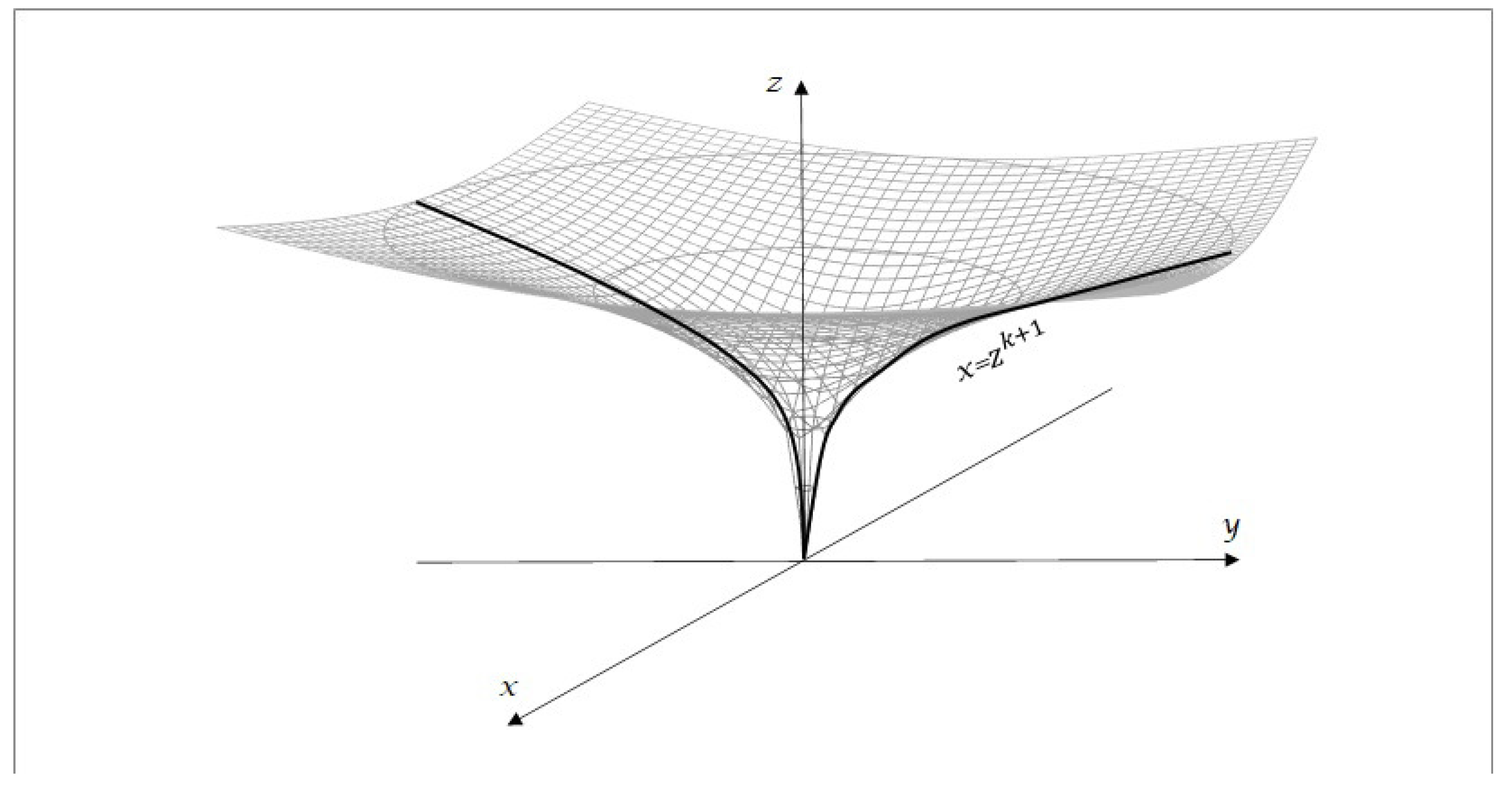
4.6. Asymptotics of the Solution of the Laplace Equation on a Manifold with an nth-Order Beak-Type Singularity

Consider the Laplace equation $\Delta u=0$ on a Riemannian two-dimensional manifold with an nth-order beak-type singularity. This means that the Riemannian metric is induced from ${\mathbb{R}}^3$ by an embedding, which is defined as a mapping of the manifold onto a surface, which is the surface of rotation of the parabola branch $y=r^n$ around the axis $\overrightarrow{0r}$ to ${\mathbb{R}}^3$.

We choose polar coordinates $(r,\phi )$ on the manifold in a neighborhood of zero and construct the asymptotics of the solution in a neighborhood of the singular point $r=0$.

The Laplace equation on a manifold has the form (see, for example, [9])

$$\frac{1}{1+n^2{r}^{2n-2}}{r}^{2n}\frac{{\partial }^{2}u}{\partial r^2}+n{r}^{2n-1}\frac{\left(n^2-n\right)r^{2n-2}+1}{{\left(1+n^2{r}^{2n-2}\right)}^2}\frac{\partial u}{\partial r}+{\left(\frac{\partial }{\partial \phi }\right)}^{2}u=0.$$

(51)

Obviously, the point $r=0$ is an irregular singular point of this equation.

Applying the method of separation of variables and substituting the function $u(r,\phi )=V\left(r\right)G\left(\phi \right)$ into Equation (51), with respect to the functions $V\left(r\right)$ and $G\left(\phi \right)$, we obtain the system of equations

$$\frac{1}{1+n^2{r}^{2n-2}}\frac{d^{2}V\left(r\right)}{d{r}^2}+n{r}^{-1}\frac{\left(n^2-n\right)r^{2n-2}+1}{{\left(1+n^2{r}^{2n-2}\right)}^2}\frac{dV\left(r\right)}{dr}-r^{-2n}\lambda V\left(r\right)=0,$$

(52)

$$\frac{d^2}{d{\phi }^2}G\left(\phi \right)=\lambda G\left(\phi \right),G\left(\phi \right)=G(\phi +2\pi ).$$

(53)

As is known, the eigenvalue of the operator corresponding to Equation (53) has the form $\lambda =k^2$, where $k\in Z$, and the eigenfunction $G_k\left(\phi \right)$ corresponding to this eigenvalue is the expansion

$$G_k\left(\phi \right)=C_{1}cosk\phi +C_{2}sink\phi ,\sqrt{\lambda }=k.$$

Let us apply Theorem 3 to the Equation (52).

If $k\ne 0$, then $m=1,k=2n>2$. It follows from Theorem 3 that the asymptotics will have the form

$$\begin{array}{c}V\left(r\right)\approx exp\left(\frac{p_1}{r^{n-1}}\right)r^{{\sigma }_1}{\displaystyle \sum _{i=0}^{\infty }}{b}_i^1{r}^i+exp\left(\frac{p_2}{r^{n-1}}\right)r^{{\sigma }_2}{\displaystyle \sum _{i=0}^{\infty }}{b}_i^2{r}^i,\hfill \\ V\left(r\right)\in E_{n-1}\left(S_R\right),\hfill \end{array}$$

where $p_i,i=1,2,$ are the roots of the polynomial

$$H_0\left(p\right)=p^2+{\left(\frac{k}{n-1}\right)}^2.$$

If $k=0$, then Equation (52) becomes

$$\frac{d^{2}V\left(r\right)}{d{r}^2}+n{r}^{-1}\frac{(n^2-n)r^{2n-2}+1}{(1+n^2{r}^{2n-2})}\frac{dV\left(r\right)}{dr}=0.$$

It follows from Theorem 3 that the asymptotics of solutions to this equation are conormal.

It is easy to show that the asymptotics in a neighborhood of zero have the form $C_{-1}/r^{n-1}$.

Denote by $V_k\left(r\right)$ the solution of the Equation (52) corresponding to the eigenvalue $\lambda =k^2$. Then, the following statement is true.

Preposition 4.

All asymptotics of solutions of the Equation (51) in the space of functions of $n-1$ exponential growth $E_{n-1}(S_R,S^1)$ can be represented as linear combinations

$$u_k(\rho ,\phi )=G_k\left(\phi \right)V_k\left(r\right),$$

where $u_k(\rho ,\phi )\in E_{n-1}(S_R,S^1)$.

5. Conclusions

The article solves the Poincaré problem for second-order ordinary differential equations, i.e., we obtain uniform asymptotics of solutions for a second-order equation with arbitrary irregular singularities. This result is of particular interest for constructing asymptotics for solutions of various equations of mathematical physics in the neighborhood of irregular singular points, which is demonstrated by the examples given in the article.

In addition, the results of this article can be applied in the theory of differential equations on manifolds with both conical and beak-like singularities. Also of particular interest is the further study of the asymptotics obtained in Theorem 1—more precisely, the question of the conditions on the coefficients of the equations that would ensure the convergence of the asymptotic series contained in the asymptotics of the solutions.

An example of such a problem, where the wave equation is considered and the convergence of the series included in the asymptotics of its solution is studied, is presented in [29].

References

1. Kondrat’ev, V.A. Boundary value problems for parabolic equations in closed regions. Tr. Mosk. Mat. Obs. 1966, 15, 400–451. [Google Scholar]
2. Kondrat’ev, V.A. Boundary value problems for elliptic equations in domains with conical or angular points. Tr. Mosk. Mat. Obs. 1967, 16, 209–292. [Google Scholar]
3. Thomé, L.W. Zür Theorie der linearen Differentialgleichungen. J. Reine Angew. Math. 1872, 74, 193–217. [Google Scholar]
4. Poincaré, H. Sur les intégrales irrégulieres des équations linéaires. Acta Math. 1886, 8, 295–344. [Google Scholar] [CrossRef]
5. Poincaré, H. Analysis of the mathematical and natural works of Henri Poincaré. In Selected Works: Mathematics; Theoretical Physics; Nauka: Moscow, Russia, 1974; Volume 3. [Google Scholar]
6. Olver, F.W.J. Asymptotics and Special Functions; (AKP Classics); A K Peters/CRC Press: Wellesley, MA, USA, 1997. [Google Scholar]
7. Sternin, B.; Shatalov, V. Borel–Laplace Transform and Asymptotic Theory. Introduction to Resurgent Analysis; CRC Press: Boca Raton, FL, USA, 1996. [Google Scholar]
8. Korovina, M. Asymptotics of Solutions of Linear Differential Equations with Holomorphic Coefficients in the Neighborhood of an Infinitely Distant Point. Mathematics 2020, 8, 2249. [Google Scholar] [CrossRef]
9. Korovina, M.V. Asymptotics of solutions of partial differential equations with higher degenerations and the laplace equation on a manifold with a cuspidal singularity. Differ. Equ. 2013, 49, 588–598. [Google Scholar] [CrossRef]
10. Kats, D.S. Computation of the asymptotics of solutions for equations with polynomial degeneration of the coefficients. Differ. Equ. 2015, 51, 1589–1594. [Google Scholar] [CrossRef]
11. Strenberg, W. Über die Asymptotische Integration von Differentialgleichungen; Verlag von Julius Springer: Berlin, Germany, 1920. [Google Scholar]
12. Coddington, E.; Levinson, N. Theory of Ordinary Differential Equations; Krieger Publishing Company: Malabar, FL, USA, 1958. [Google Scholar]
13. Cesari, L. Asymptotic Behavior and Stability Problems in Ordinary Differential Equations; Springer: Berlin/Heidelberg, Germany, 1963. [Google Scholar]
14. Korovina, M.V.; Shatalov, V.E. Differential equations with degeneration and resurgent analysis. Differ. Equ. 2010, 46, 1267–1286. [Google Scholar] [CrossRef]
15. Korovina, M.V. Existence of resurgent solutions for equations with higher-order degeneration. Differ. Equ. 2011, 47, 346–354. [Google Scholar] [CrossRef]
16. Ecalle, J. Cinq applications des fonctions resurgentes. Publ. Math. D’Orsay 1984, 84T62, 110. [Google Scholar]
17. Schulze, B.-W.; Sternin, B.; Shatalov, V. Asymptotic Solutions to Differential Equations on Manifolds with Cusps; Max-Planck-Institut fur Mathematik: Bonn, Germany, 1996; p. MPI 96-89. [Google Scholar]
18. Schulze, B.-W.; Sternin, B.; Shatalov, V. An Operator Algebra on Manifolds with Cusp-Type Singularities. Ann. Glob. Anal. Geom. 1998, 16, 101–140. [Google Scholar] [CrossRef]
19. Sternin, B.Y.; Shatalov, V.E. Differential Equations in Spaces with Asymptotics on Manifolds with Cusp Singularities. Differ. Equ. 2002, 38, 1764–1773. [Google Scholar] [CrossRef]
20. Sciarra, G.; dell’Isola, F.; Hutter, K. Dilatational and compacting behavior around a cylindrical cavern leached out in a solid-fluid elastic rock salt. Int. J. Geomech. 2005, 5, 233–243. [Google Scholar] [CrossRef] [Green Version]
21. dell’Isola, F.; Gouin, H.; Seppecher, P. Radius and surface tension of microscopic bubbles by second gradient theory. Comptes Rendus Acad. Sci. 1995, 320, 211–216. [Google Scholar]
22. dell’Isola, F.; Gouin, H.; Rotoli, G. Nucleation of spherical shell-like interfaces by second gradient theory: Numerical simulations. Eur. J. Mech. B Fluids 1996, 15, 545–568. [Google Scholar]
23. Matevossian, O.A. Solutions of exterior boundary-value problems for the elasticity system in weighted spaces. Sb. Math. 2001, 192, 1763–1798. [Google Scholar] [CrossRef]
24. Matevossian, H.A. On solutions of mixed boundary value problems for the elasticity system in unbounded domains. Izv. Math. 2003, 67, 895–929. [Google Scholar] [CrossRef]
25. Matevossian, H.A. On the polyharmonic Neumann problem in weighted spaces. Complex Var. Elliptic Equ. 2019, 64, 1–7. [Google Scholar] [CrossRef]
26. Matevossian, H.A. Asymptotics and uniqueness of solutions of the elasticity system with the mixed Dirichlet–Robin boundary conditions. Mathematics 2020, 8, 2241. [Google Scholar] [CrossRef]
27. Migliaccio, G.; Matevossian, H.A. Exterior biharmonic problem with the mixed Steklov and Steklov-type boundary conditions. Lobachevskii J. Math. 2021, 42, 1886–1899. [Google Scholar] [CrossRef]
28. Korovina, M.V.; Matevossian, H.A.; Smirnov, I.N. Uniform Asymptotics of Solutions of the Wave Operator with Meromorphic Coefficients. Appl. Anal. 2021. [Google Scholar] [CrossRef]
29. Korovina, M.V.; Matevossian, H.A.; Smirnov, I.N. On the Asymptotics of Solutions of a Boundary Value Problem for the Hyperbolic Equation at t. Lobachevskii J. Math. 2021, 42, 3684–3695. [Google Scholar] [CrossRef]
Figure 1. Cone.
Mathematics 10 02465 g001
Figure 2. Beak.
Mathematics 10 02465 g002
Figure 3. Contour γ ˜ and domain Ω ˜ R , ε .
Mathematics 10 02465 g003
Publisher’s Note: MDPI stays neutral with regard to jurisdictional claims in published maps and institutional affiliations.