Article

Exponentially-Fitted Fourth-Derivative Single-Step Obrechkoff Method for Oscillatory/Periodic Problems

by
Ashiribo Senapon Wusu
1,2,†,
Olusola Aanu Olabanjo
2,3,*,† and
Manuel Mazzara
4,†
1
Department of Mathematics, Lagos State University, Lagos 102101, Nigeria
2
Africa Center of Excellence for Innovative and Transformative STEM Education (ACEITSE), Lagos State University, Lagos 102101, Nigeria
3
Department of Mathematics, Morgan State University, Baltimore, MD 21251, USA
4
Institute of Software Development and Engineering, Innopolis University, Innopolis 420500, Russia
*
Author to whom correspondence should be addressed.
These authors contributed equally to this work.
Mathematics 2022, 10(14), 2392; https://doi.org/10.3390/math10142392
Submission received: 12 June 2022 / Revised: 26 June 2022 / Accepted: 1 July 2022 / Published: 7 July 2022
(This article belongs to the Special Issue Advanced Numerical Analysis and Scientific Computing)

Abstract

:
The quest for accurate and more efficient methods for solving periodic/oscillatory problems is gaining more attention in recent time. This paper presents the construction and implementation of a family of exponentially-fitted Obrechkoff methods using a six-step flowchart discussed in the literature. A single-step Obrechkoff method involving terms up to the fourth derivative was used as the base method. We also present the stability and convergence properties of the constructed family of methods. Two numerical examples were used to illustrate the performance of the constructed methods.

1. Introduction

Ordinary Differential Equations (ODEs) that exhibit pronounced oscillatory or periodic behaviour in their solutions are often encountered in fields such as chemistry, engineering, electronic, mechanics and astrophysics [1,2,3]. Many of the classical methods for solving prominent classes of problems in ODE have been developed using only monomials as a basis [1,4,5,6,7,8]. In [9], the authors used a hybrid method to examine the direct solution of higher order (second, third and fourth order) initial value problem (IVP) of ordinary differential equations. However, in practice, many classical methods usually perform poorly when applied to problems with pronounced periodic or oscillatory behaviour in their solution [3,10,11]. This is due to the fact that for better accuracy to be achieved, a very small step size would be required with corresponding decrease in performance, especially in terms of efficiency [1]. One way to overcome this barrier is to adapt classical methods for such problems. The adaptation which is called “exponential/trigonometric fitting” involves the replacement of some of the highest order monomials of the basis by exponentials or trigonometric [3,11].Detailed analysis of the oscillation–preserving behaviour of some existing RKN–type methods were analysed from the point of view of geometric integration in [12]. Authors in [13] presented surveys on recent advances in the allied challenges of discretizing highly oscillatory ordinary differential equations and computing numerical quadrature of highly oscillatory integrals. They also attempted to sketch the mathematical foundations of a general approach to these issues [13] .
A pioneering work in the use of exponentially–fitted formulae for differential equations was conducted by [14]. The authors in [14] constructed integration formulae which contains free parameters - chosen so that a given function exp ( q ) where q is real, satisfies the integration formulae exactly. The proposed method in [14] was on a one-step formulae, however, in [15], A-stable fourth order exponentially-fitted formulae based on a linear two-step formula was derived. Using the concept proposed in [15], the author in [16] proposed a Multiderivative Linear Multistep Method (MLMM) with k = 1 in the second derivative formulae. Many authors have proposed specially adapted Runge–-Kutta (RK) algorithms to solve this class of problems [17,18,19,20]. In this direction, exponentially–fitted RK (EFRK) methods which integrate exactly first–order systems whose solutions can be expressed as linear combinations of functions of the form { exp ( λ t ) , exp ( λ t ) } or { cos ( ω t ) , sin ( ω t ) } were introduced in [21,22]. The construction of an implicit trigonometrically-fitted single-step method with a second derivative using trigonometric basis function was proposed in [23].
In this work, we used the six–step flowchart described in [3] to construct a class of exponentially–fitted single-step fourth-derivative Obrechkoff methods suitable for solving
y = f ( x , y ) , x x 0 , X , y ( x 0 ) = y 0 .

2. Construction of Method

A classical fourth-derivative single-step Obrechkoff method for solving the first order initial value problem (1) can generally be written as
y j + 1 = a 0 y j + h b 1 f j + 1 + b 0 f j + h 2 c 1 f j + 1 + c 0 f j + h 3 d 1 f j + 1 + d 0 f j + h 4 e 1 f j + 1 + e 0 f j
where a 0 , b 0 , b 1 , c 0 , c 1 , d 0 , d 1 , e 0 and e 1 are coefficients to be determined. Here, we present the construction of the exponentially-fitted variants of (2) using the six-step flowchart described in [3]. Following the six-step flowchart, the corresponding linear difference operator L [ h , a ] is obtained as
L [ h , a ] y ( x ) = y ( x + h ) a 0 y ( x ) h b 1 y ( x + h ) + b 0 y ( x ) h 2 c 1 y ( x + h ) + c 0 y ( x ) h 3 d 1 y ( x + h ) + d 0 y ( x ) h 4 e 1 y ( x + h ) + e 0 y ( x )
where a : = ( a 0 , b 0 , b 1 , c 0 , c 1 , d 0 , d 1 , e 0 , e 1 ) . Step II of the procedure requires that we get the maximum value of M such that the algebraic system
L m * ( a ) = h m L [ h , a ] x m | x = 0 = 0 | m = 0 , 1 , 2 , , M 1
can be solved. The above results in
L 0 * ( a ) = 1 a 0 = 0
L 1 * ( a ) = b 0 b 1 + 1 = 0
L 2 * ( a ) = 2 b 1 2 c 0 2 c 1 + 1 = 0
L 3 * ( a ) = 3 b 1 6 c 1 6 d 0 6 d 1 + 1 = 0
L 4 * ( a ) = 4 b 1 12 c 1 24 d 1 24 e 0 24 e 1 + 1 = 0
L 5 * ( a ) = 5 b 1 20 c 1 60 d 1 120 e 1 + 1 = 0
L 6 * ( a ) = 6 b 1 30 c 1 120 d 1 360 e 1 + 1 = 0
L 7 * ( a ) = 7 b 1 42 c 1 210 d 1 840 e 1 + 1 = 0
L 8 * ( a ) = 8 b 1 56 c 1 336 d 1 1680 e 1 + 1 = 0
and the algebraic system is compatible when M = 9 . In addition, the solution only results in the coefficients of the associated classical method to be adapted. To exponentially fit the associated classical method, we proceed to step III of the six–step flowchart and obtain expressions for G + ( Z , a ) and G ( Z , a ) which are respectively defined as
G + ( Z , a ) = 1 2 E 0 * ( z , a ) + E 0 * ( z , a )
G ( Z , a ) = 1 2 z E 0 * ( z , a ) E 0 * ( z , a )
where E 0 * ( ± z , a ) = e ω x L [ h , a ] e ± ω x and Z = z 2 . The expressions for G + ( Z , a ) and G ( Z , a ) are respectively obtained as
G + ( Z , a ) = a 0 + sinh Z b 1 Z d 1 Z 3 / 2 + cosh Z c 1 Z e 1 Z 2 + 1 c 0 Z e 0 Z 2
G ( Z , a ) = cosh Z b 1 d 1 Z b 0 + sinh Z c 1 Z e 1 Z 3 / 2 + 1 Z d 0 Z
where ω , the frequency of oscillation is real or imaginary, z = ω h = ω h . (For the trigonometric case, i.e., ω is imaginary, we choose z = ω h = i μ h , i.e., z 2 = μ 2 h 2 = Z .)
To implement step IV, consider the reference set of M functions:
1 , x , , x K , exp ( ± ω x ) , x exp ( ± ω x ) , , x P exp ( ± ω x )
with K + 2 P = M 3 . Since for our method M = 9 , we have five possibilities, which we shall respectively refer to as S1, S2, S3, S4 and S5:
  • S1: K = 8 , P = 1 , the classical case with the set
    1 , x , x 2 , x 3 , x 4 , x 5 , x 6 , x 7 , x 8
  • S2: K = 6 , P = 0 , the mixed case with the set
    1 , x , x 2 , x 3 , x 4 , x 5 , x 6 , exp ( ± ω x )
  • S3: K = 4 , P = 1 , the mixed case with the set
    1 , x , x 2 , x 3 , x 4 , exp ( ± ω x ) , x exp ( ± ω x )
  • S4: K = 2 , P = 2 , the mixed case with the set
    1 , x , x 2 , exp ( ± ω x ) , x exp ( ± ω x ) , x 2 exp ( ± ω x )
  • S5: K = 0 , P = 3 , the mixed case with the set
    1 , exp ( ± ω x ) , x exp ( ± ω x ) , x 2 exp ( ± ω x ) , x 3 exp ( ± ω x )
In order to get the corresponding coefficients of the method associated with each case, we implement step V of the algorithm by solving the algebraic system
L k * = 0 , 0 k K , G ( p ) ± ( Z , a ) = 0 , 0 p P
and the coefficients of the methods associated with each case are respectively obtained as follows:
S1 :: (K,P) = (8,−1)
a 0 = 1 b 0 = b 1 = 1 2 c 0 = c 1 = 3 28 d 0 = d 1 = 1 84 e 0 = e 1 = 1 1680
Equation (17) gives the coefficients of the classical method associated with Equation (2).
S2 :: (K,P) = (6,0)
a 0 = 1 b 0 = b 1 = 1 2 c 0 = c 1 = z 4 120 sinh z 2 5 z z 2 12 cosh z 2 10 z 2 z 2 + 12 sinh z 2 6 z cosh z 2 d 0 = d 1 = z 4 60 z 2 720 sinh z 2 + 360 z cosh z 2 120 z 2 z 2 + 12 sinh z 2 6 z cosh z 2 e 0 = e 1 = z z 2 + 60 cosh z 2 12 z 2 + 10 sinh z 2 120 z 2 z 2 + 12 sinh z 2 6 z cosh z 2
S3 :: (K,P) = (4,1)
a 0 = 1 b 0 = b 1 = 1 2 c 0 = c 1 = z 4 12 z 2 + z 2 36 z sinh ( z ) + 96 cosh ( z ) 96 12 z 2 z 2 + z sinh ( z ) 4 cosh ( z ) + 4 d 0 = d 1 = 4 z 2 + 6 + z 2 + 24 cosh ( z ) 9 z sinh ( z ) 6 z 2 z 2 + z sinh ( z ) 4 cosh ( z ) + 4 e 0 = e 1 = z 4 + 12 z 2 z 2 + 48 z sinh ( z ) + 12 z 2 + 4 cosh ( z ) 48 12 z 4 z 2 + z sinh ( z ) 4 cosh ( z ) + 4
S4 :: (K,P) = (2,2)
a 0 = 1 b 0 = b 1 = 1 2 c 0 = c 1 = sinh z 2 2 z 3 + 21 z + 24 sinh ( z ) 18 z 2 cosh z 2 3 z sinh 3 z 2 2 z 2 2 z 2 + 1 cosh z 2 2 z sinh z 2 cosh 3 z 2 d 0 = d 1 = z 3 cosh z 2 + sinh z 2 3 z 2 + 3 z sinh ( z ) 16 cosh ( z ) + 16 z 3 2 z 2 + 1 cosh z 2 2 z sinh z 2 cosh 3 z 2 e 0 = e 1 = sinh z 2 2 z 3 21 z + 12 sinh ( z ) + 6 z 2 cosh z 2 z sinh 3 z 2 2 z 4 2 z 2 + 1 cosh z 2 2 z sinh z 2 cosh 3 z 2
S5 :: (K,P) = (0,3)
a 0 = 1 b 0 = b 1 = 2 4 z 3 6 2 z 2 + 1 sinh ( z ) + 2 z 2 + 3 z cosh ( z ) 6 z + 3 sinh ( 2 z ) z z 2 + 3 z 2 2 z 2 + 3 z sinh ( z ) + 6 z 2 cosh ( z ) 3 sinh 2 ( z ) c 0 = c 1 = 2 z 4 3 z 2 ( 4 cosh ( z ) + 3 ) + 9 sinh 2 ( z ) + 12 z sinh ( z ) z 2 z 2 + 3 z 2 2 z 2 + 3 z sinh ( z ) + 6 z 2 cosh ( z ) 3 sinh 2 ( z ) d 0 = d 1 = 2 2 z 3 ( cosh ( z ) + 2 ) + 6 sinh ( z ) 3 sinh ( 2 z ) 6 z ( cosh ( z ) 1 ) z 3 z 2 + 3 z 2 2 z 2 + 3 z sinh ( z ) + 6 z 2 cosh ( z ) 3 sinh 2 ( z ) e 0 = e 1 = z 4 + 2 z 3 sinh ( z ) + z 2 ( 3 6 cosh ( z ) ) 3 sinh 2 ( z ) + 6 z sinh ( z ) z 4 z 2 + 3 z 2 2 z 2 + 3 z sinh ( z ) + 6 z 2 cosh ( z ) 3 sinh 2 ( z )
As expected, the exponentially fitted variants reduce to the classical method as z 0 .

3. Error Analysis :: Local Truncation Error (lte)

The leading term of the local truncation error (lte) for the exponentially-fitted method with respect to the basis functions
1 , x , , x K , exp ( ± ω x ) , x exp ( ± ω x ) , , x P exp ( ± ω x )
is of the form
l t e E F ( t ) = ( 1 ) P + 1 h M L K + 1 * ( a ( Z ) ) ( K + 1 ) ! Z P + 1 D K + 1 ( D 2 ω 2 ) P + 1 y ( x )
with K, P and M satisfying the condition K + 2 P = M 3 , [3].
For the five methods constructed in this work, the leading terms of the local truncation error are obtained as follows:
  • S1 :: ( K , P ) = ( 8 , 1 )
    l t e E F ( t ) = h 9 y ( 9 ) ( x ) 25,401,600
  • S2 :: ( K , P ) = ( 6 , 0 )
    l t e E F ( t ) = h 9 20 z z 2 + 42 cosh z 2 z 4 + 180 z 2 + 1680 sinh z 2 100,800 z 4 z 2 + 12 sinh z 2 6 z cosh z 2 × u ( 9 ) ( t ) ω 2 u ( 7 ) ( t )
  • S3 :: ( K , P ) = ( 4 , 1 )
    l t e E F ( t ) = h 9 720 z 8 z 2 + z sinh ( z ) 4 cosh ( z ) + 4 × 2880 240 z 2 + 24 z 4 + z 6 24 z 4 + 50 z 2 + 120 cosh ( z ) + z z 4 + 240 z 2 + 2880 sinh ( z ) × y ( 9 ) ( x ) 2 ω 2 y ( 7 ) ( x ) + ω 4 y ( 5 ) ( x )
  • S4 :: ( K , P ) = ( 2 , 2 )
    l t e E F ( t ) = h 9 12 z 9 2 z 2 + 1 cosh z 2 2 z sinh z 2 cosh 3 z 2 × z 3 2 z 2 + 85 cosh z 2 + z 3 cosh 3 z 2 + 2 sinh z 2 192 + 99 z 2 + 7 z 4 192 cosh ( z ) + 108 z sinh ( z ) ) 18 z 2 sinh 3 z 2 × y ( 9 ) ( x ) 3 ω 2 y ( 7 ) ( x ) + 3 ω 4 y ( 5 ) ( x ) ω 6 y ( 3 ) ( x )
  • S5 :: ( K , P ) = ( 0 , 3 )
    l t e E F ( t ) = h 9 4 4 z 3 6 2 z 2 + 1 sinh ( z ) + 2 z 2 + 3 z cosh ( z ) 6 z + 3 sinh ( 2 z ) z z 2 + 3 z 2 2 z 2 + 3 z sinh ( z ) + 6 z 2 cosh ( z ) 3 sinh 2 ( z ) + 1 z 8 × y ( 9 ) ( x ) 4 ω 2 y ( 7 ) ( x ) + 6 ω 4 y ( 5 ) ( x ) 4 ω 6 y ( 3 ) ( x ) + ω 8 y ( x )

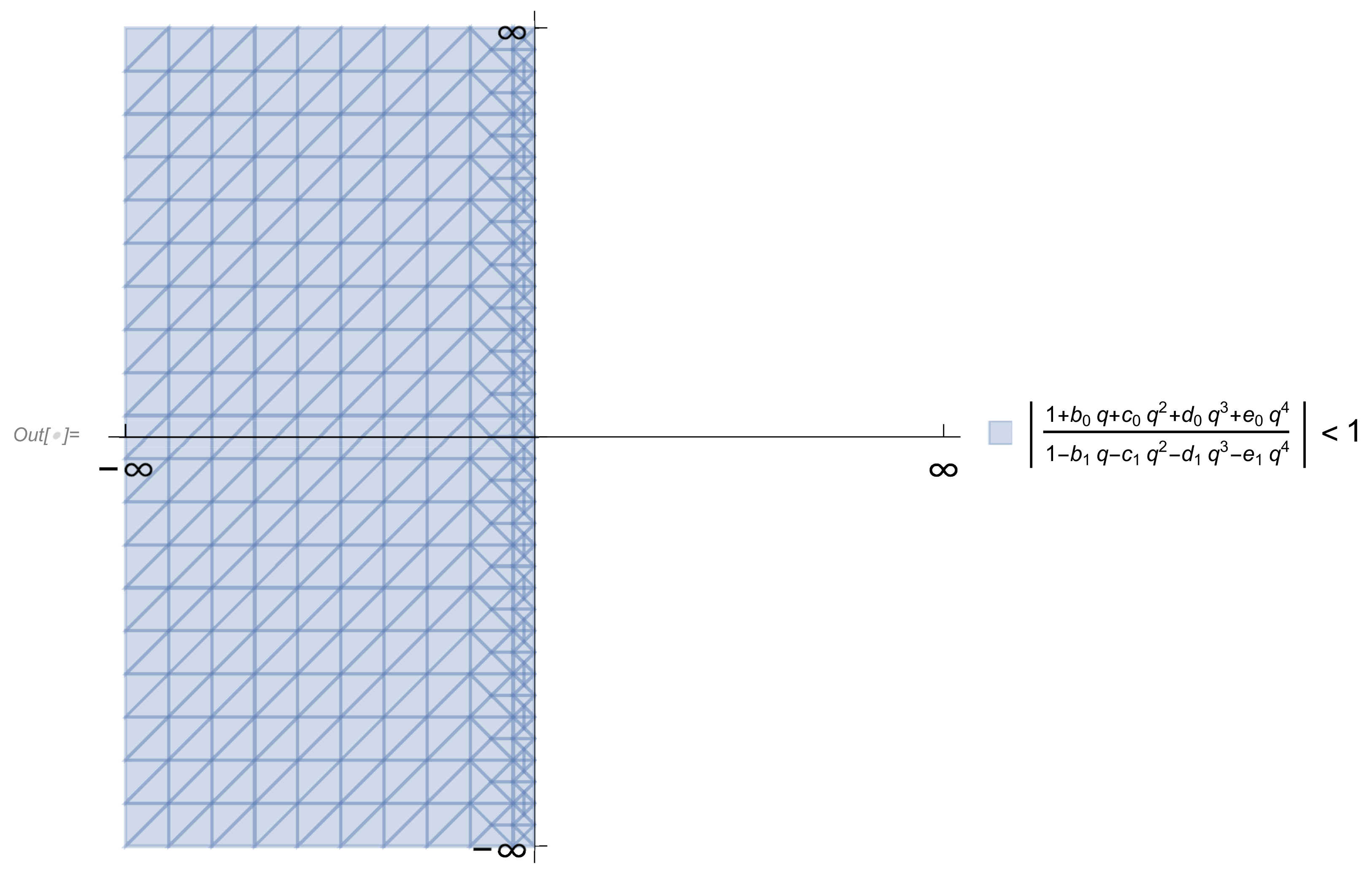
4. Convergence and Stability Analysis

Theorem 1
(Dahlquist Theorem). The necessary and sufficient conditions for a linear multistep method to be convergent are that it be consistent and zero-stable [4].
Dahlquist Theorem (1) also holds true for exponetially-fitted-based algorithms but the concepts of consistency and stability have to be adapted since their coefficients are no longer constants.
Definition 1.
An exponentially-fitted method associated with the fitting space (22) is said to be of exponential order q, relative to the frequency ω if q is the maximum value of M such that the algebraic system L m * ( a ) = 0 | m = 0 , , M 1 is compatible [3].
Definition 2.
A linear multistep method is said to be consistent if it has order P 1 [1,4].
Since the order of the constructed method, M = 9 1 for all the constructed schemes, the consistency requirement is satisfied. Hence, the constructed schemes are all consistent.
Definition 3.
The method Equation (2) is zero stable if no root of the first characteristic polynomial has modulus greater than one and if every root with modulus one is simple [1,2].
In order to establish the stability of (2), we apply Equation (2) to the test problems y = λ y and obtain the stability function R ( q ) , of the class of methods as
y n + 1 y n = R ( q ) = 1 + b 0 q + c 0 q 2 + d 0 q 3 + e 0 q 4 1 b 1 q c 1 q 2 d 1 q 3 e 1 q 4 , with q = λ h .
Definition 4.
A region of absolute stability is a region in the complex plane, throughout which R ( q ) < 1 . Any closed curve defined by R ( q ) = 1 is an absolute stability boundary. In addition, any interval ( α , β ) of the real line is said to be the interval of absolute stability if the method is stable for all q ( α , β ) [1,4].
The absolute stability regions for all the methods constructed in this work are the same and given in Figure 1.
From Figure 1, it can be seen that stability region of the methods contains the entire left half plane, hence they are all A-stable and have their absolute stability interval as , 0 .

5. Numerical Results

In this section, we considered two test problems. The constructed methods are implemented on these test problems and the obtained results were compared with those of the classical eighth-order Runge-Kutta (RK-8) method.

5.1. Problem 1

The first test problem considered in this work is the initial value problem given as
y y = 0.001 cos x , y ( 0 ) = 1 , y = 0
with exact solution
y ( x ) = cos x + 0.0005 x sin x
This problem was studied in [24,25]. Using different stepsizes, we implement the constructed methods on this problem and present the maximum absolute errors in Table 1.
For this problem, the exponentially fitted methods gave better results compared with their classical counterpart and the Runge–Kutta method as seen from Table 1.

5.2. Problem 2

The inhomogeneous equation
y + 100 y = 99 sin x , y ( 0 ) = 1 , y = 11 .
with exact solution
y ( x ) = sin ( x ) + sin ( 10 x ) + cos ( 10 x )
is considered as the second test case. This problem has also been studied by [24,26]. The constructed methods were implemented on it with different stepsizes and the results obtained were also compared with those of the Runge-Kutta method. The table of maximum absolute errors is given in Table 2.
Again, the exponentially fitted methods gave better results compared with their classical counterpart and the Runge-Kutta method as seen from Table 2.

6. Conclusions

An exponentially-fitted one-step fourth-derivative Obrechkoff method for oscillatory problems was constructed. The new methods are self-starting and of algebraic order eight. The stability and convergence properties of the constructed method were analysed and we showed that the new methods are A-stable. The results obtained from the numerical examples show that the new methods are suitable for solving periodic/oscillatory problems.

Author Contributions

Conceptualization, A.S.W. and O.A.O.; methodology, A.S.W. and O.A.O.; software, A.S.W. and M.M.; validation, A.S.W. and O.A.O.; formal analysis, A.S.W. and O.A.O.; investigation, A.S.W. and O.A.O.; resources, A.S.W. and O.A.O.; data curation, A.S.W. and O.A.O.; writing—original draft preparation, A.S.W. and O.A.O.; writing—review and editing, M.M. and A.S.W.; visualization, A.S.W. and O.A.O.; supervision, M.M. and A.S.W. All authors have read and agreed to the published version of the manuscript.

Funding

This research received no external funding.

Institutional Review Board Statement

Not applicable.

Informed Consent Statement

Not applicable.

Data Availability Statement

Not applicable.

Conflicts of Interest

The authors declare no conflict of interest.

References

  1. Lambert, J.D. Computational Methods in ODEs; Wiley: New York, NY, USA, 1973. [Google Scholar]
  2. Lambert, J. Numerical Methods for Ordinary Differential Systems; Wiley: New York, NY, USA, 1991. [Google Scholar]
  3. Ixaru, L.; Vanden Berghe, G. Exponential Fitting: Mathematics and Its Applications; Kluwer Academic Publishers: Alphen aan den Rijn, The Netherlands, 2004. [Google Scholar]
  4. Butcher, J. Numerical Methods for Ordinary Differential Equations; Wiley: New York, NY, USA, 2008. [Google Scholar]
  5. Akanbi, M.A. On 3-stage Geometric Explicit Runge-Kutta Method for Singular Autonomous Initial Value Problems in Ordinary Differential Equations. Computing 2011, 92, 243–263. [Google Scholar] [CrossRef]
  6. Wusu, A.S.; Okunuga, S.A.; Sofoluwe, A.B. A Third-Order Harmonic Explicit Runge-Kutta Method for Autonomous Initial Value Problems. Glob. J. Pure Appl. Math. 2012, 8, 441–451. [Google Scholar]
  7. Wusu, A.S.; Akanbi, M.A. A Three-Stage Multiderivative Explicit Runge-Kutta Method. Am. J. Comput. Math. 2013, 3, 121–126. [Google Scholar] [CrossRef] [Green Version]
  8. Wusu, A.S.; Akanbi, M.A.; Fatimah, B.O. On the Derivation and Implementation of a Four Stage Harmonic Explicit Runge-Kutta Method. Appl. Math. 2015, 6, 694–699. [Google Scholar] [CrossRef] [Green Version]
  9. Abolarin, O.E.; Adeyefa, E.; Kuboye, J.O.; Ogunware, B.G. A Novel Multiderivative Hybrid Method for the Numerical Treatment of Higher Order Ordinary Differential Equations. Al Dar Res. J. Sustain. 2020, 4, 43–56. [Google Scholar]
  10. Simos, T.E. An exponentially-fitted Runge-Kutta method for the numerical integration of initial-value problems with periodic or oscillating solutions. Comput. Phys. Commun. 1998, 115, 1–8. [Google Scholar] [CrossRef]
  11. Vanden Berghe, G.; Daele, M. Exponentially-fitted Stomer/Verlet methods. J. Numer. Anal. Ind. Appl. Math. 2006, 1, 241–255. [Google Scholar]
  12. Wu, X.; Wang, B.; Mei, L. Oscillation-preserving algorithms for efficiently solving highly oscillatory second-order ODEs. Numer. Algorithms 2021, 86, 693–727. [Google Scholar] [CrossRef]
  13. Iserles, A. On the Numerical Analysis of Rapid Oscillation. In CRM Proceedings and Lecture Notes; Centre for Mathematical Sciences: Cambridge, UK, 2004; pp. 1–15. [Google Scholar]
  14. Liniger, W.S.; Willoughby, R.A. Efficient Integration methods for Stiff System of ODEs. SIAM J. Numer. Anal. 1970, 7, 47–65. [Google Scholar] [CrossRef]
  15. Jackson, L.W.; Kenue, S.K. A Fourth Order Exponentially Fitted Method. SIAM J. Numer. Anal. 1974, 11, 965–978. [Google Scholar] [CrossRef]
  16. Cash, J.R. On exponentially fitting of composite multiderivative Linear Methods. SIAM J. Numer. Anal. 1981, 18, 808–821. [Google Scholar] [CrossRef]
  17. Coleman, J.P.; Duxbury, S.C. Mixed collocation methods for y = f(x;y). J. Comput. Appl. Math. 2000, 126, 47–75. [Google Scholar] [CrossRef] [Green Version]
  18. Avdelas, G.; Simos, T.E.; Vigo-Aguiar, J. An embedded exponentially-fitted Runge-Kutta method for the numerical solution of the Schrodinger equation and related periodic initial-value problems. Comput. Phys. Commun. 2000, 131, 52–67. [Google Scholar] [CrossRef]
  19. Franco, J.M. An embedded pair of exponentially fitted explicit Runge-Kutta methods. J. Comput. Appl. Math. 2002, 149, 407–414. [Google Scholar] [CrossRef] [Green Version]
  20. Bettis, D.G. Runge-Kutta algorithms for oscillatory problems. J. Appl. Math. Phys. (ZAMP) 1979, 30, 699–704. [Google Scholar] [CrossRef]
  21. Vanden Berghe, G.; Meyer, H.D.; Daele, M.V.; Hecke, T.V. Exponentially-fitted explicit Runge-Kutta methods. Comput. Phys. Commun. 1999, 123, 7–15. [Google Scholar] [CrossRef]
  22. Vanden Berghe, G.; Meyer, H.D.; Daele, M.; Hecke, T. Exponentially fitted Runge-Kutta methods. J. Comput. Appl. Math. 2000, 125, 107–115. [Google Scholar] [CrossRef] [Green Version]
  23. Ngwane, F.F.; Jator, S.N. Trigonometrically–fitted second derivative method for oscillatory problems. SpringerPlus 2014, 3, 304. [Google Scholar] [CrossRef] [Green Version]
  24. Zhai, W.; Chen, B. Exponentially Fitted RKNd Methods for Solving Oscillatory ODEs. Adv. Math. 2013, 42, 393–404. [Google Scholar]
  25. Franco, J. Exponentially fitted explicit Runge-Kutta-Nystrom methods. J. Comput. Appl. Math. 2004, 167, 1–19. [Google Scholar] [CrossRef] [Green Version]
  26. Van de Vyver, H. A Runge-Kutta-Nystrom pair for the numerical integration of perturbed oscillators. Comput. Phys. Commun. 2005, 167, 129–142. [Google Scholar] [CrossRef]
Figure 1. Region of absolute stability for the constructed methods.
Mathematics 10 02392 g001
Table 1. Maximum absolute error for constructed methods on Section 5.1 with step-size h = 2 i π , i = 0 , 1 , 2 , 3 .
iRK-8 ( K , P ) = ( 8 , 1 ) ( K , P ) = ( 6 , 0 ) ( K , P ) = ( 4 , 2 ) ( K , P ) = ( 2 , 1 ) ( K , P ) = ( 0 , 3 )
08.256847 × 10 1 1.701678 × 10 5 0.0000000.0000000.0000002.220446 × 10 16
15.921881 × 10 3 1.485065 × 10 5 1.516774 × 10 8 1.160079 × 10 13 4.170189 × 10 14 9.992007 × 10 16
29.221257 × 10 5 6.125912 × 10 8 6.400131 × 10 11 1.488434 × 10 11 6.878617 × 10 12 7.895672 × 10 13
31.154806 × 10 6 2.425554 × 10 10 3.548604 × 10 11 1.3173 × 10 9 3.317455 × 10 10 7.396323 × 10 11
Table 2. Maximum absolute error for constructed methods on Section 5.2 with step-size h = 2 i π , i = 0 , 1 , 2 , 3 , 4 , 5 .
iRK-8 ( K , P ) = ( 8 , 1 ) ( K , P ) = ( 6 , 0 ) ( K , P ) = ( 4 , 2 ) ( K , P ) = ( 2 , 1 ) ( K , P ) = ( 0 , 3 )
02.385689 × 10 27 2.3854026.994405 × 10 15 5.77316 × 10 15 1.210143 × 10 14 3.719247 × 10 14
12.779917 × 10 37 2.4100111.507892 × 10 7 1.467305 × 10 4 4.454081 × 10 3 7.805366
21.036922 × 10 39 2.4137782.714209 × 10 7 4.764676 × 10 5 6.398771 × 10 3 1.120104
31.466513 × 10 12 2.377447 × 10 1 4.035951 × 10 10 4.450952 × 10 8 4.873151 × 10 6 5.310473 × 10 4
44.728532 × 10 1 1.336235 × 10 3 1.392109 × 10 12 1.123486 × 10 10 1.137188 × 10 8 1.153992 × 10 6
55.249947 × 10 3 5.711746 × 10 6 1.162043 × 10 11 6.347695 × 10 11 3.808664 × 10 11 4.012365 × 10 9
Publisher’s Note: MDPI stays neutral with regard to jurisdictional claims in published maps and institutional affiliations.

