
Learning-Oriented QoS- and Drop-Aware Task Scheduling for Mixed-Criticality Systems
by
 , ,
, ,
Behnaz Ranjbar
1,2,* ,
,
Hamidreza Alikhani
2,
Bardia Safaei
2,
Alireza Ejlali
2,* and
Akash Kumar
1,* 1
CFAED, Technische Universität (TU) Dresden, 01069 Dresden, Germany
2
Department of Computer Engineering, Sharif University of Technology, Tehran 11365-11155, Iran
*
Authors to whom correspondence should be addressed.
Computers 2022, 11(7), 101; https://doi.org/10.3390/computers11070101
Submission received: 17 May 2022
/
Revised: 9 June 2022
/
Accepted: 16 June 2022
/
Published: 22 June 2022
(This article belongs to the Special Issue Human Understandable Artificial Intelligence)
Abstract
:In Mixed-Criticality (MC) systems, multiple functions with different levels of criticality are integrated into a common platform in order to meet the intended space, cost, and timing requirements in all criticality levels. To guarantee the correct, and on-time execution of higher criticality tasks in emergency modes, various design-time scheduling policies have been recently presented. These techniques are mostly pessimistic, as the occurrence of worst-case scenario at run-time is a rare event. Nevertheless, they lead to an under-utilized system due to frequent drops of Low-Criticality (LC) tasks, and creation of unused slack times due to the quick execution of high-criticality tasks. Accordingly, this paper proposes a novel optimistic scheme, that introduces a learning-based drop-aware task scheduling mechanism, which carefully monitors the alterations in the behaviour of the MC system at run-time, to exploit the generated dynamic slacks for reducing the LC tasks penalty and preventing frequent drops of LC tasks in the future. Based on an extensive set of experiments, our observations have shown that the proposed approach exploits accumulated dynamic slack generated at run-time, by 9.84% more on average compared to existing works, and is able to reduce the deadline miss rate by up to 51.78%, and 33.27% on average, compared to state-of-the-art works.
1. Introduction
Modern embedded systems in various applications such as automotive, avionics, and medical devices, are getting more complex due to integrating many functions with different criticality levels into a common platform [1,2,3]. In these systems (called Mixed-Criticality (MC) systems), the correct execution of all tasks with higher criticality levels (HC tasks) must be guaranteed in any situation, while low-criticality tasks (LC tasks) can be penalized in emergency situations [2,4,5]. For instance, drones are an MC system, where the engine control (i.e., the function that ensures the safe execution of the operation) is an HC task, and the process of recording a video (which is its main mission) is considered as an LC task [6,7].
From the MC task analysis perspective, the MC systems are designed to support the worst-case scenario in any situation and guarantee the safety of an MC system. Therefore, HC tasks are analyzed with optimistic and pessimistic assumptions to obtain different Worst-Case Execution Times (WCETs) [8,9]. At run-time, if the execution time of an HC task exceeds its optimistic WCET (i.e., requires additional resources), the system switches from low-criticality (LO) mode to high-criticality (HI) mode (also called emergency mode), and all HC tasks will be scheduled based on their pessimistic WCETs to guarantee the system’s safety. In the HI mode, it is possible that some or all LC tasks are dropped to ensure the correct execution of the HC tasks [2,5,10], which reduces the result’s quality. However, there are some issues in designing MC systems in a pessimistic manner, including (1) under-utilization at run-time, and (2) frequent drop of LC tasks in the HI mode. In the latter case, considering a constant value for the drop rate (a parameter that specifies the minimum jobs that must be executed between two consecutive drops of an LC task) may have a negative impact on the execution of other tasks and consequently cause the system not to execute its mission correctly. This is despite the fact that many of the existing MC scheduling algorithms have employed this approach by analyzing the tasks at design-time and specified the LC tasks that must be dropped if the system switches its mode to HI. In these studies, the dropping policies remain unchanged during run-time, which causes the system to be under-utilized due to the unnecessary dropping of some LC tasks. Therefore, it is necessary to consider the run-time behaviour of MC systems along with the assumptions that have been made at design-time (i.e., monitoring the state of the system and controlling the task dropping in the HI mode), to improve the utilization and Quality of Service (QoS) for LC tasks [2].
Many studies have concentrated on improving the timing behaviour of these systems in both design- and run-time phases. From a design-time point of view, different scheduling policies have been presented to guarantee the real-time constraints of HC tasks while improving the LC tasks’ QoS in the HI mode [7,10,11]. However, most of these approaches design the MC system pessimistically, which causes the system to be under-utilized at run-time. In addition, their policies unnecessarily drop LC tasks, which degrades their service requirements in favor of HC tasks in the HI mode. In addition, some run-time approaches improve the QoS by proposing a new scheduling policy or exploiting the dynamic slacks [4,8,12]. However, due to the lack of complete observation of the MC system’s behaviour, the decision may be ineffective, and there may be no guarantee of meeting the LC tasks’ service requirements.
To this end, we propose SOLID, a novel optimistic mechanism that reduces the number of drops for the LC tasks by observing the system’s behavior changes at run-time. This goal has been achieved by exploiting the generated dynamic slacks in the decision-making process for the online task dropping to execute more LC tasks in the HI mode and enhance their schedulability. Since we are not aware of the amount of generated dynamic slacks during run-time in advance, Machine-Learning (ML) approaches can be employed as a management technique for the prediction. Therefore, utilizing ML techniques as part of the SOLID has enabled it to partially exploit the dynamic slack to improve the QoS for the LC tasks in the HI mode. In these schemes, the learner finds the optimum drop rate for the LC tasks, prevents frequent drops in HI mode, and consequently reduces their deadline miss rate. We also extend the proposed mechanism, which is lenient in applying the learned drop-rate data to the scheduler. Accordingly, the main contributions of this article are:
- Presenting a novel adaptive technique with high QoS to schedule MC tasks at run-time.
- Proposing a learning-based drop-aware MC task scheduling mechanism, called SOLID, to improve the QoS by exploiting the generated dynamic slacks rigorously, during run-time with no HC tasks’ deadline misses.
- Extending the proposed mechanism (SOLID) to a mechanism that uses accumulated dynamic slack moderately, called LIQUID.
The proposed approaches were analyzed with an extensive set of evaluations. Experiments show that the proposed approaches can exploit the generated dynamic slacks by 9.84% on average and reduce the deadline miss rate by 33.27% on average compared to existing studies.
The rest of this paper is organized as follows: We first review the related studies in Section 2. The system models and preliminaries are discussed in Section 3. In Section 4, we present a motivational example along with a problem statement to explain the problem to the readers better. The proposed approaches is discussed in detail in Section 5, and finally we analyze and conclude the experiments in Section 6 and Section 7, respectively.
2. Related Works
The majority of the existing studies in the context of MC systems have focused on proposing techniques for managing different aspects of the system, e.g., task schedulability and QoS at design-time. However, a few efforts also been conducted to manage these parameters at run-time. Although researchers in [2] give a comprehensive study in the field of task scheduling techniques and QoS improvement in MC systems in run-time and design-time phases, this section provides an overview of the existing studies, which are very close to the proposed approach. In addition, as part of our review, we also introduce some learning-based approaches in the field. Table 1 summarizes these works with their respective properties, such as considering single/multi-core (S/M-Core) platform, MC/non-MC task Model, run-/design-time approach, Using of ML, and QoS improvement (offline/online-manner). In this table, None means that the researchers do not consider the property in their work.
Since most MC systems are safety-related and real-time, the task schedulability in terms of QoS is typically analyzed at design-time to guarantee the correct execution of tasks before their deadlines to prevent catastrophic damages while the system is operating. Row 1 of Table 1 introduces some studies which improve the QoS of LC tasks in the HI mode while investigating the task scheduling feasibility. The authors in [5,7,9,11,13] have focused on MC systems to guarantee the LC tasks’ QoS in the worst-case scenario (up to their WCETs). In these approaches, executing the minimum number of instances (i.e., dropping fewer instances of LC tasks) in the HI mode is ensured. However, all these approaches are applicable at design-time to guarantee the minimum QoS. This is despite the fact that the system does not operate in the worst-case scenario at run-time in most cases. Therefore, the guaranteed minimum QoS of LC tasks could be improved. Although authors in [7] have proposed an approach to enhance the QoS by determining a constant drop rate parameter for LC tasks and guaranteeing their schedulability in the HI mode based on the defined parameter, their presented scheme has been analyzed in the worst-case scenario of tasks’ execution, while there may exist significant amount of idle time in the processor at run-time, which could be used for improving the QoS of LC tasks. Some articles in the field of MC systems such as [14,15,16] have presented the scheduling algorithms for multi-core processors, which can also improve the LC tasks’ QoS (row 2). However, these methods have been presented to guarantee the tasks’ deadlines in the worst-case scenario at design-time.
From the MC task scheduling on multi-core processors perspective at run-time, Sigrist et al. [17] (row 3) have studied the recent task scheduling mechanisms, and evaluated the effect of run-time overheads, such as task execution monitoring, overrunning detection, and mode switching. However, they have not improved the task scheduling and QoS at run-time. To improve the LC tasks’ QoS at run-time, researchers in [4,8,12,18,19] have presented the run-time adaptability mechanisms by exploiting the accumulated dynamic slack to execute more LC tasks in the HI mode (row 4). In [4], a run-time schedulability analysis has been presented, and LC tasks are executed in free slack time if the conditions are met. Researchers in [18] have also presented an effective solution for reducing the number of mode switches and consequently LC task dropping by using the generated dynamic slack for executing HC tasks when they overrun. Bate et al. [19] have also proposed a protocol that handles mode switches and ensures that LC tasks are executed more frequently. However, in such three works, some LC tasks may be dropped frequently and continuously when the system switches to the HI mode, which is unacceptable in any situation in some MC systems. In addition, all dynamic slack is not exploited in [12] properly since the algorithm only uses the dynamic slack generated by HC tasks’ execution. Fixed-priority Earliest-Deadline-First (EDF) scheduling algorithm has been used in the presented algorithm of [8], which is less efficient compared to the common EDF [23], such as EDF with Virtual Deadline (EDF-VD). These methods may drop LC tasks frequently due to improper system design and insufficient dynamic slack.
When considering the system’s property optimization at run-time, there exist several studies which have proposed ML-based methods to manage the task schedulability to improve the performance (executing more tasks in the system) [20,21,22] (row 5). However, these approaches could not manage different operational modes, including (1) scheduling all tasks to be executed successfully before their deadlines and (2) guaranteeing and improving the minimum QoS when the system switches to the HI mode. The downsides of the previous approaches have motivated us to study the MC systems’ behaviour at run-time, and propose an ML-based approach to improve the LC tasks’ QoS in multi-core platforms.
3. System Model
This paper focuses on a multi-core platform, consisting of c homogeneous cores . The system executes MC applications, in which analogous to many state-of-the-art studies [4,5,7,9,24], we consider a set of n independent periodic MC tasks . Each task is represented as , where is the criticality level of the task. We consider a dual-criticality system, where tasks can be high-critical ( = HC), or low-critical ( = LC). In these dual-criticality systems, each task has two Worst-Case Execution Times (WCETs), i.e., optimistic (), and pessimistic (). For each task , if = HI, then we have , and if = LO, then . In addition, denotes the deadline of the task , which is equal to its period [7]. represent the virtual deadline () which provides a higher priority for HC task , while the tasks are scheduled in the LO mode. Details regarding the definition and computation of the virtual deadlines are explained in [10]. As mentioned earlier, dropping all LC tasks in the HI mode is not acceptable in industrial applications. Thus, researchers in [7,11] have defined a drop rate parameter for each LC task to be employed in the HI mode. This parameter specifies the minimum jobs that must be executed between two consecutive drops of an LC task. It is represented as (s,m)-deadline, where at most, s jobs could be dropped out of m jobs [11]. The authors in [7] have considered a specific case with s = 1 and m = . Accordingly, we also utilize the same definition as in [7,11], for the case that s = 1. In this definition, if = 1, it means that all jobs of would be dropped in the HI mode. As we used several symbols and notations, a list of them is provided in Table 2 for easy following.
MC System Operational Model: Initially, the system begins its operation in the LO mode, where all of the LC and HC tasks must be executed before their deadlines. If the execution time of at least one HC task exceeds its optimistic WCET (), the system switches to the HI mode. In the HI mode, all of the HC tasks are considered to be executed up to their pessimistic WCET (). Therefore, LC tasks will be scheduled based on their defined drop rate values in favor of HC tasks; therefore, all these HC tasks can be executed correctly before their deadlines. Finally, in case there are no remaining ready HC tasks in the queue of the cores, the system will safely switch back to the LO mode and continue its operation [3,4,5,9,11,24].
4. Motivational Example and Problem Statement
The main motivation for our proposed method comes from the fact that the MC systems are typically designed in a way that they are obliged to map and schedule the tasks in the worst-case scenario at design-time, before the system starts its operation. This is despite the fact that the application’s QoS, system utilization, and deadline miss rate of LC tasks in case of HI mode switching will be affected while the application is executing at run-time. Indeed, the properties of MC systems can be improved according to the status of the tasks’ execution over time. To support this claim, let us consider a simple drone application composed of five tasks . For the sake of simplicity, assume that the application runs on a single-core processor. The tasks’ timing parameters have been shown in Table 3. The period of task () is equal to the task’s relative deadline. In addition, since the EDF-VD algorithm is used to schedule the task, a virtual deadline (, which is less than the relative deadline) is needed to be defined for HC tasks (the detail of how it is computed, has been explained in [10]).
In this example, , , and are HC tasks and and are LC tasks. Each task function is determined in Table 3. Dropping an LC task, such as , could be acceptable in HI mode, but it should not frequently happen due to its responsibility. For instance, in multimedia tasks, e.g., , the maximum drop rate (i.e., the rate of skipping the videos) must be guaranteed when the MC systems are designed to satisfy the customers. More specifically, the minimum QoS of LC tasks must be guaranteed in the HI mode. Hence, most of the previously MC scheduling algorithms have been designed based on the maximum drop rate of LC tasks before the system starts its operation. Furthermore, these rates are kept constant during the tasks’ operation at run-time when the system switches to the HI mode. Figure 1 illustrates four task scheduling approaches, including (1) Method of [10], a design-time approach that drops all LC tasks in the HI mode, (2) Methods of [7,11], the design-time approaches, which drop LC tasks based on their drop-rates in the HI mode, (3) Method of [7,11], investigating their approaches at run-time, and finally, (4) Proposed method in this paper. According to this figure, each task has several jobs, released at the beginning of its period. Therefore, a released job (j) of task is shown by with an upward arrow.
Figure 1a depicts the task scheduling procedure under the principles of the proposed mechanism in [10]. Accordingly, assume that all of the tasks should comply with their specified time budget ( in the LO mode and in the HI mode) to be executed correctly. This figure shows that the system switches to the HI mode by overrunning. In this figure, the jobs of (), and () are dropped twice in the HI mode, which is not acceptable in many MC applications. Figure 1b shows a scheduling mechanism which can schedule LC tasks in the HI mode [7,11]. Accordingly, the LC tasks are dropped based on their predefined drop-rate parameters. In this scenario, only , and will not be executed in the HI mode. As it can be seen, the presented approaches in [7,11] enable the MC system to schedule LC tasks in the HI mode, and improve the LC tasks’ QoS. Nevertheless, their design principles in the MC systems are all considered in the worst-case scenario of the task execution, which is not optimal. At run-time, the tasks are typically finished earlier than their WCET in most cases, and then some dynamic slack would be created. As an example, Figure 1c shows the run-time behavior of the system, where some dynamic slack has been generated, and the tasks have finished their execution earlier. Therefore, other tasks could start their execution earlier, and the core would spend more time in the idle mode, compared to the scheduling mechanism depicted in Figure 1b.
Based on what we have learned, it is recommended that the system should be able to manage its behavior during run-time, to minimize the drop rate of some LC tasks in the HI mode. As a result of this action, the QoS will be enhanced, e.g., less video will be skipped, which is desirable. Figure 1d represents the task scheduling at run-time, where the dynamic slack has been used to minimize the drop rate when the system is in the HI mode (such as and which are not dropped). Although we are not aware of the amount of dynamic slack in advance, they could be exploited to improve the QoS.
Motivated by the above mentioned example, prior to explaining the details of our novel scheduling technique, we define the constraints, and the objective function, as follows:
Deadline Constraints: Each HC task with the WCET , running on core must finish its execution ( is the finish time of task ) correctly before its deadline () in both LO and HI modes. In addition, all LC tasks must finish their execution before their deadlines in LO mode. In addition, in case of switching to the HI mode, most LC tasks must finish their execution before their deadlines according to their drop rate .
Objective Function: We optimize the MC system QoS at run-time by maximizing the LC tasks’ QoS in the system by utilizing the following objective function: Maximize or Minimize , where DMR is deadline miss rate and the QoS is defined as the percentage of executed LC tasks in the HI mode to all LC tasks [7,25,26] (, where is the number of all LC tasks and is the number of executed LC tasks before their deadlines), which can be optimized by optimizing their drop rates () (). The QoS is computed at the end of each hyper-period based on the number of non-executed LC tasks. Hence, the hyper-period is the Least Common Multiple (LCM) of all tasks’ periods.
The problem is how to use the generated dynamic slack at run-time to maximize the QoS for satisfying the timing constraint. While we are not aware of the amount of dynamic slack in the future, it is possible to turn it into a partially controllable entity at run-time to optimize the intended objective. This could be done by using ML techniques. Therefore, this paper proposes a novel learning-based and drop-aware scheduling for MC tasks running on a multi-core platform. As discussed below, we utilize our newly proposed technique to use the generated dynamic slack at run-time to achieve better performance and QoS.
5. Proposed Method in Detail
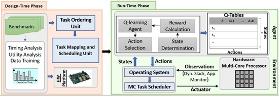
In this section, we present SOLID; a novel Strict learning-Oriented Quality-of-Service- and Drop-aware task scheduling mechanism for MC systems, to apply in the run-time phase. As illustrated in Figure 2, our proposed approach contains a design-time, and a run-time phase. Application characteristics, architecture information, and QoS metric are counted as inputs and scheduled tasks, and QoS improvement are the outputs. Accordingly, we first need to analyze the task schedulability at design-time based on their characteristics (Section 5.1) to guarantee the minimum QoS requirement for the system. Therefore, we use the approach of [7,11] to ensure the task schedulability and the minimum QoS. In addition, to manage the resources of the system architecture, we should also map the tasks at design-time in the multi-core platform. Finally, we exploit our newly introduced learning-based optimization mechanism at run-time (Section 5.2). In the following, we explain the details of the proposed approach in each of these phases.
5.1. An Overview of the Design-Time Approach
This section focuses on task mapping and scheduling at design-time. According to Figure 2, the timing properties of tasks are obtained by running real-world benchmarks on a hardware platform (more details about the benchmarks and the platform are provided in Section 6). We map the tasks on the multi-core platform and validate the schedulability test using the tasks’ parameters in the worst-case scenario. In addition, as part of ML technique employment, since embedded MC systems are the target systems, some aspects of the learning process, data, and model training are conducted at design-time, with robust offline learning techniques in the worst-case scenarios. More detail is discussed in Section 5.2.2. Since the generated dynamic slack is used to execute more LC tasks in the case of mode switches, we study multi-core platforms to see how the core and task ordering policies affect the system’s outputs. Nevertheless, there are two main issues in task mapping the tasks [27]: (1) Core selection, which we have decided to use broadly heuristic techniques, e.g., First-Fit (FF), Best-Fit (BF), and Worst-Fit (WF), (2) Order of tasks to be mapped. Accordingly, we use the Decreasing-Criticality (DC) and Decreasing-Utilization (DU) heuristic, which indicates that the tasks are sorted in decreasing order of their criticality levels or utilization.
In order to schedule the tasks on cores, a well-known scheduling algorithm, EDF-VD, is used. Since this algorithm has been widely studied in previous studies, we mention this algorithm briefly in this and the next sub-sections. To test the task schedulability during the mapping, the EDF-VD scheduling algorithm conditions are employed [7,10]. Generally, the mapped tasks on the same core are schedulable if all HC tasks can be executed correctly before their deadlines in any condition, and all of the LC tasks could be schedulable in the LO mode. In the HI mode, LC tasks can be scheduled based on their defined drop rates (i.e., the LC tasks’ minimum QoS can be guaranteed in the worst-case scenario), as discussed in Section 3. As a result, a set of tasks is schedulable under the EDF-VD in both operational modes on each core if the following necessary and sufficient conditions are met [7]. Equation (2) presents the maximum utilization bounds for MC systems in both LO and HI modes that it must be less than one to let the tasks be schedulable under EDF-VD at run-time and also the system switch safely between the modes. Since the LC tasks must be dropped in the HI mode based on their drop-rate values with no effect on HC tasks’ execution, Equation (3) presents the sufficient condition for executing both HC and LC tasks in this HI mode (The information and the proofs of these conditions have been explained in detail in [7]).
where denotes the total utilization of the tasks with the same criticality level l, mapped on a same core in the mode k, and is the hyper-period of the mapped tasks on a core.
5.2. Run-Time Approach: Employment of SOLID
The main goal of SOLID is to enhance the LC tasks’ QoS (i.e., minimizing the number of dropped LC tasks) under the mode switching situation by exploiting the dynamic slacks at run-time, with no deadline misses of HC tasks in any situation. This capability has been brought to SOLID by exploiting learning-based techniques. Note that the learning algorithm and the scheduling algorithm are independent, and we do not use learning techniques to schedule the tasks. In fact, the proposed approach is independent of the task scheduling algorithm, and the learning process is used to improve the QoS independent of scheduling tasks. Here, any scheduling algorithm can be applied to the tasks; however, this learning-based task scheduling mechanism is built upon the EDF-VD algorithm. To guarantee the schedulability of HC tasks in both LO and HI modes, when the system begins its operation, HC tasks are scheduled based on their virtual deadlines, and the LC tasks are scheduled based on their actual deadlines. In the HI mode, all HC tasks are scheduled based on their actual deadlines, while the LC tasks will be scheduled according to the SOLID scheduling principles. It should be mentioned that although the learning process can be done independently of the scheduler, its timing overhead to obtain the new drop rate values of LC tasks may be significant in real-time systems. Therefore, we can consider its timing overhead while checking the task schedulability. The details of the timing overhead of the learning process and how it is considered in schedulability test are presented in Section 6.3. In this section, we first overview the employed reinforcement learning technique as part of our proposed mechanism; then, we fully describe SOLID, based on the mentioned learning technique.
5.2.1. Learning-Based System Properties Optimization
Reinforcement Learning (RL) can be applied to systems with a considerable dynamism through trial and error. By using the historical data and learning from past events, it can improve the performance based on the dynamic changes [28]. The Q-learning/SARSA technique, which is recently been used in many emerging applications, such as robotics, and Unmanned Aerial Vehicles (UAV) [29,30], uses the RL technique to perform the run-time management/optimization of the system properties in single or multi-core processors. The general Q-learning/SARSA technique consists of the three main components [31,32], including: (1) a discrete set of states , (2) a discrete set of actions , and (3) reward function R. The states and actions determine the rows and columns of the Q-table of the learning-based algorithm, respectively (shown in Figure 2). The algorithm collects the current state , and determines the next action (). A value-based algorithm is represented with for each state-action pair in the Q-table. The Q-values are updated based on the corresponding computed reward in every iteration. The Q-values are calculated according to Equation (4) [31,32,33], which is based on the SARSA learning algorithm [34,35]. The algorithm learns the optimal action in every state, and this process is repeated until a predefined convergence criterion is met. Note that SARSA and Q-learning are two RL methods and tend to optimize the results in the end. However, SARSA is an online policy, while Q-learning is offline. These two different policies lead to different next action selection and Q-table updating. Since the proposed approach is composed of offline and online phases, and it is critically important to have a robust offline training technique for considering the worst-case scenarios before the system gets operational at run-time, SARSA would be the best choice for finding the optimum value (because there is no urgency at design-time to find the optimum value). Therefore, SARSA can explore most of the states in the data training.
where , and represent the state and action at time t, respectively. Furthermore, and indicate their values at time . determines the learning rate of overriding the old data in the table by the new acquired data (). R is the reward function, and is the discount rate to determine the importance of the future reward (). In this work, we set the values of to 0.2, and to 0.5. These values are determined based on a wide range of experiments, which are set to obtain the best improvement.
5.2.2. SOLID Optimization
In order to maximize the QoS in MC systems, here we propose our learning-based approach for the operation of the system in HI mode. It should be mentioned that the time of the system mode changes and how long the system stays in each mode are unknown. As a result, the system encounters dynamic slacks with varying lengths, which would result in different actions in the intended mode. In SOLID, the agent controller has been designed to maximize the QoS by decreasing the LC tasks’ drop rates (i.e., drop less often) when the system switches to the HI mode. Note that no action is required in the learning process if the dynamic slack is too small. In order to update the Q-table, we check the generated dynamic slack at the end of each hyper-period. Based on the available slack, we update the Q-table, and decisions are taken (i.e., the new drop-rate value is determined). It should be mentioned that since we target real-time embedded MC systems, we conduct some parts of the learning process, data, and model training for the Q-table at design-time with robust offline learning techniques in the worst-case scenarios. The reason is that the learned Q-table can be utilized to quickly determine the optimal actions based on the system state and also reduce the probability of bad decisions. Then, by using this data and what the learning algorithm learns from this training phase at design-time and also the obtained historical data at run-time, the algorithm improves its prediction process as time passes. In the following, we first explain the system state, action determination, and reward computation for the learning process to generate the Q-table values. Then, we present the proposed approach in detail.
System State Determination: There are various criteria for determining the system states. In our proposed scheme, for the Q-table, the states of the system depend on the available CPU utilization and dropped LC task in a period. To represent the states in a formal way, for each state , , where . Both utilization and dropped tasks are normalized to their maximum value (shown by ). We also define 10 ranges to determine the percentage of missed tasks to all tasks. As an example, consider as the utilization range (). Therefore, we have , which indicates the variation in the rate of dropped LC tasks for the fixed utilization range. In each iteration, according to the unused utilization and the rate of dropped tasks in the previous hyper-period, the current state is determined for the Q-table. Here, we select an optimal action for the current system state. Thus, the system can gradually reach the optimal state.
Learning Action Determination: There are various methods for determining the optimal action according to the state . In this paper, the well-known -greedy policy has been exploited, in which the dynamic policy is used for adjusting [36]. In -greedy policy, random action is selected from the actions set with the probability of , i.e., the best action is selected with the largest Q-value with the probability of . We first use a dynamic -greedy policy with the value of at design-time to prevent the probability of the learning algorithm being stuck at few Q-values. Accordingly, we can accelerate the learning process. Afterward, the fixed -greedy policy is used with the value of at run-time to ensure that the system reaches the optimum state and chooses the best action based on the Q-values, which has the maximum value. The action space in the Q-table illustrates an increase/decrease in a LC task’s drop-rate (,.., ). It should be noted that the minimum values of drop-rates are equal to the initial values that is used for schedulability analysis at design-time.
Reward Computation: In general, the reward indicates how well the learning algorithm performed in the previous step. This approach calculates the reward at the end of each hyper-period based on the available dynamic slack. Hence, when there is less accumulated dynamic slack at the end of the hyper-period, it means more core capacity () has been used on that hyper-period for the core cr. The considered reward function for the Q-table shows in Equation (5), which is based on the generated dynamic slack at the end of each period.
The reward function considers three scenarios. If the utilization falls into the unsafe zone that may cause deadline violation, the decision will be penalized. Unsafe zone means the utilization may increase more than one, where EDF-VD cannot guarantee the timeliness of all tasks. Accordingly, it results in a negative value (, where and has a constant value) for the reward function, which decreases the Q-value in Equation (4), i.e., reduces the probability of choosing it in the future. In Equation (5), we set the value of equal to 100 to highly impact the value of the reward function in a negative manner. In addition, since our goal is to use all of the accumulated dynamic slack to optimize the system property, would be the optimum case for the reward function (presented in Equation (2)). However, since there may be some errors in the first phases of the learning technique, we consider the upper bound of core utilization () to be less than one (). In fact, it can be equal to , where has an extremely low positive value, such as . Hence, we consider a value less than the maximum core utilization as the core utilization limit to never let it violate the threshold.
Actual Execution Time Predictor Policy: Due to releasing several jobs of a task in each hyper-period, the execution times of jobs may be different in each hyper-period. We have to predict the execution times to compute the core utilization () in Equation (2), according to the previous run-time tasks’ execution times. This prediction is based on the following equation, where is the predicted execution time of task for hyper-period , is the regression coefficient, and is the error (presents how different the estimated value is from the actual one). In the evaluations, x is assumed to be eight.
Figure 2 depicts our proposed learning-based drop-aware task scheduling mechanism. It consists of the environment, i.e., hardware platform, the agent, and its interaction with the operating system and the applications. This learning-based property improvement technique has been designed for a system based on its states, and action determination algorithms discussed earlier. The scheduler schedules the tasks based on the EDF-VD on multi-core processors at run-time. At the end of each hyper-period, the accumulated dynamic slack, and the number of dropped LC tasks in the HI mode are observed. The proposed learning phase decides how to increase/decrease the LC tasks’ drop-rates based on the Q-table and reward function value. The major goal of SOLID is to use most of the created slack-time and consequently maximize the core utilization by optimizing the LC-tasks’ drop-rates. In the learning process, the agent observes the state at a time period instance , computes the award, updates the Q-table, and performs an action. The action (a) is selected from the predefined action set in the specified Q-Table (, where k is the maximum number of actions corresponding to each table). The chosen action is applied for the next time period (). After decoding the actions for the HI mode by the operating systems, based on the new LC task drop rates, the policies of the task scheduling and LC tasks dropping will be updated in the case that the system mode switches to the HI mode.
To guarantee meeting the deadline of HC tasks, although we try our best effort and define the hard margin to avoid missing the deadlines, it could happen for the EDF algorithm in the worst-case scenario that the core is fully utilized and all tasks are executed up to their WCETs at run-time, while some LC tasks’ drop-rates were increased according to learned data. It may lead to some deadline misses for HC tasks. As a result, SOLID is strict in applying the learned data into the scheduler to ensure meeting the deadlines in the worst-case scenario. The scheduler in SOLID approach always considers the initial drop-rate values () and drops LC tasks based on them in the HI mode. To apply the leaned data, the dynamic slack is detected at run-time. When an HC task finishes its execution early, a dynamic slack is generated due to the early completion. Based on the learned drop rate values, the scheduler in SOLID releases the LC jobs to execute in this generated dynamic slack. Therefore, LC tasks are executed more times (drop fewer) by exploiting the slack time generated only from the early completion of HC tasks’ executions and improving the QoS in the HI mode. Although it introduces an extra workload for the system, it causes to prevents affecting the early LC tasks’ releases on HC tasks’ timeliness. We require judicious slack management to determine whether it is feasible to release an LC job at a time point.
However, in order to be lenient in applying the learned drop-rate data into the scheduler, we extend SOLID to LIQUID, which uses accumulated dynamic slack moderately to improve QoS.
5.3. LIQUID Approach
In LIQUID (Learning-Based Quality-of-Service- and Drop-Aware MC Task Scheduling Mechanism), such as what we proposed in SOLID, the proposed learning algorithm operates independently of the scheduler. However, in despite of SOLID, LIQUID applies the learned data into the scheduler with no restriction and taking care of generated dynamic slack by HC tasks. The scheduler in LIQUID approach always considers the learned drop-rate values, and LC tasks are dropped based on them in the case of mode switches.
To make both approaches explicit, consider a task with , which means one job would be dropped among three jobs in the HI mode. If the learned drop-rate after a hyper-period is equal to , it means one job would be dropped among six jobs. Therefore, the rate of task dropping would be half in comparison with the initial value. In fact, one more job among six jobs would be scheduled and executed. LIQUID always considers for the LC task when the system switches to the HI mode. While in SOLID, considers for task . If there is sufficient accumulated dynamic slack at run-time to execute based on the learned , the task is released. In this work, we exploit and adapt the early-release policy, presented in [27], which is an effective slack management technique in MC systems and based on a known mechanism, called wrapper-task mechanism [37,38].
Algorithm: Algorithm 1 illustrates the pseudo-code of the run-time approach, including both scheduling and learning procedures at the same time. As inputs, the algorithm takes the tasks and their characteristics (e.g., WCET, criticality level, period, and drop-rate, period), the hardware platform, and its major configuration information (such as the number of cores), and finally, the minimum QoS requested by the tasks. In addition, since a part of the learning process is done at design-time, the Q-table is obtained and taken as input. On the other hand, improvements in the LC tasks’ QoS and the scheduled tasks are defined as outputs at the end (Time). At each time, the scheduler checks the status of the tasks in each core, whether they are overrun or not, which results in mode switching (line 4). This unit also checks the periods of tasks whether they would be released or not. All tasks on every core are scheduled based on the EDF-VD algorithm (line 5). In the case of mode switches to the HI, the LC tasks are dropped based on their defined drop rate values to guarantee the correct execution of HC tasks. In lines 7–11, the number of dropped LC tasks are counted to be used in the learning process. If the system switches back to the LO mode, a parameter (CountDrop) for each task, which counts the number of released LC tasks in the HI mode, is set to zero (lines 13–14). Besides, there is a function (line 17) that checks whether the output of each task is ready. When ready, the task is removed from the core queue, and the generated dynamic slack is added to the slack array (lines 17–18). The learning process is conducted at the end of each hyper-period (lines 19–29). In this process, the number of dropped LC tasks in the HI mode and the accumulated dynamic slack are used to determine the state (line 20). As mentioned earlier, since the Greedy policy is used, if a random number is less than , a random action is selected (line 22, exploration phase of learning process); otherwise, an action with the maximum value in the Q-table is chosen for that particular state (line 23, exploitation phase of learning process). Based on the chosen action, a new drop-rate is determined for the task (line 25). Consequently, the reward function updates the Q-table (lines 26–27). Note that if an embedded system is kept running for a long time, although the system is in the exploitation phase over time, which uses the learned data, as can be illustrated from the policy, there is still a slight chance to learn if there is any pattern shift.
| Algorithm 1 Proposed Learning-Based Scheme at Run-Time |
| Input:Task Set, Cores, Q-table |
| Output:QoS, Scheduled Tasks |
| 1: procedure LEARNING-BASED QoS OPTIMIZATION() |
| 2: for each cr in Cores do = 0; |
| 3: for t = 1 to Time do |
| 4: [,] = TaskStatusCheck(Tasks) |
| 5: [] = EDF-VD (, Cores) |
| 6: if = = 1 then |
| 7: for each released LC do |
| 8: + = 1; |
| 9: if mod(,) = = 0 then + = 1; |
| 10: end if |
| 11: end for |
| 12: else |
| 13: for each do = 0; |
| 14: end for |
| 15: end if |
| 16: = TaskOutputCheck(Tasks) |
| 17: if = = 1 then = |
| 18: end if |
| 19: if mod(t,) = = 0 then |
| 20: State = Deter-State (,) |
| 21: k = rand (1); //(0<k<1) //ϵ-Greedy Policy |
| 22: if then = argrand |
| 23: else = argmax |
| 24: end if |
| 25: Set the new task’s drop-rate based on the action |
| 26: R = CompReward () // Equation (5) |
| 27: //Equation (4) |
| 28: = 0; = 0; |
| 29: end if |
| 30: end for |
| 31: end for |
| 32: end procedure |
6. System Setup and Evaluation
The experiments are conducted on a Linux-based machine equipped with 1.4 GHz, a quad-core processor, and 16GB of memory. Since there are no real-life MC benchmarks to conduct the experiments, the major related studies have evaluated their proposed techniques by using synthetic task sets [7,8,9,17]. However, in addition to synthetic task sets, we use various real-time tasks included in MiBench benchmark suite [39] for the evaluations. Besides, we analyze and compare the efficiency of proposed approaches against various methods [7,8,9,11,12] in terms of schedulability, run-time QoS improvement, and available free slack at the end of a hyper-period. Researchers in [7,11] use the EDF-VD scheduling algorithm while dropping LC tasks in the HI mode according to the drop-rate parameter, without using the run-time adaptability. In [9], the QoS is improved by degrading the WCETs of LC tasks in the HI mode. In [8,12], the run-time adaptability is employed by exploiting the accumulated dynamic slack. A dynamic reservation-based task scheduling algorithm has been presented in [12] to minimize the deadline miss rate by using the dynamic slack, which is generated by the early completion of HC tasks. In [8], a fixed-priority EDF is used, and the QoS is improved by precising the LC tasks’ WCETs in the HI mode.
6.1. Evaluation with Real-Life Benchmarks
As mentioned, MiBench benchmark suite [39] has been used, which is dedicated to applications such as automotive, network, and telecommunications. More specifically, we consider the benchmarks of ‹edge›, ‹smooth›, ‹epic›, and ‹corner› as the LC tasks and ‹qsort›, ‹insertsort›, ‹matrixmult›, ‹dijkstra›, ‹bitcount›, and ‹FFT› as the HC tasks in our system evaluations. To achieve their execution times, these benchmarks have been executed on the ODROID XU4 hardware platform. We consider the utilization of the tasks in the [0.05,0.1] interval (to be able to execute more tasks in a core), and the period/deadline of the tasks are computed according to the utilization and WCET values [7,10]. More detail on WCETs values has been reported in [40]. In addition, the values of the drop-rate () for the LC tasks are randomly generated between 1 and its maximum value (which has been set to four in our experiments), based on the uniform distribution. Table 4 represents the normalized number of deadline misses (NDM), normalized to method of [9]), and the QoS of different methods. As shown in this table, at run-time, LIQUID has provided the maximum QoS and the minimum NDM compared to the other methods. In addition, since the methods of [7,11] have also presented a design-time drop-aware approach to not drop LC tasks frequently when the system switches to the HI mode, the QoS has a high value (and low NDM value) compared to the other existing studies. Although the proposed techniques in [8,12] are run-time approaches, which improve the QoS, they are not well designed to exploit better from run-time profit. However, since [12] uses the EDF-VD algorithm, which well utilizes the system’s capacity compared to the other existing scheduling algorithms, e.g., fixed-priority, and also exploits the generated dynamic slack, it provides better results in terms of QoS and NDM in comparison with [8].
In addition, as mentioned in Section 3, we define a drop-rate value for each of the LC tasks in the HI mode. At run-time, these values are optimized based on the generated dynamic slacks. In our experiments, the drop-rate values for 4 LC tasks have been updated from to , which has led to QoS improvement at run-time.
We evaluate the effects of different partitioning algorithms and task ordering policies on the LC tasks’ QoS during the run-time phase for the mentioned real task set with the utilization of , where c is the number of cores. We have run the experiment 50 times and reported the average results in this section. As mentioned in Section 5.1, three heuristics of FF, BF, and WF are used to select a core for the process of task mapping. In addition, we have also employed two task ordering policies, i.e., Decreasing-Utilization (DU), and Decreasing-Criticality (DC), while mapping the tasks on the cores. Since the result of BF is very close to the result of FF, we only illustrate the results for BF and WF in this section. Figure 3 represents the QoS of the LC tasks at run-time, normalized to BF-DC policy, with different numbers of cores while using our proposed LIQUID technique. The results show that the DC policy for task ordering performs better than the DU policy under both BF and WF heuristics. The reason for having better results under the BF heuristic is an uneven distribution of tasks among the cores. It means that the first cores are selected to execute most of the HC tasks, while the rest of the cores are chosen to execute the LC tasks. Therefore, by switching the system to the HI mode, there is less force to drop LC tasks in favor of HC tasks. In addition, achieving better results under the WF heuristic with the DC task ordering policy for the LC and HC tasks is due to the more evenly task distribution among the cores. Therefore, more amount of dynamic slack would be generated, which could be used to execute the LC tasks and improve the QoS if the system switches its mode. In addition, using the WF heuristic for selecting the cores to map a task has a better result than using the BF heuristic under the DU task ordering policy. This is due to more task balancing among all cores, while the BF heuristic aims to schedule the tasks under the minimum required number of cores. As a result, while employment of the WF heuristic leads to a uniform utilized core, due to scheduling more evenly task distribution on cores, the system may frequently switch to the HI mode, and consequently, more LC tasks would be dropped in the HI mode.
6.2. Evaluation with Synthetic Task Sets
Now we investigate the efficiency of LIQUID and SOLID under the presence of synthetic task sets. To generate synthetic task sets, analogous to [5,9,10], we consider dual-criticality task sets that are generated for various system utilization bounds ( = ). We randomly add tasks to the task set to increase , (where is the number of cores) until it reaches a given threshold in the [0.05,1] interval, with steps of 0.05. In addition, the periods of tasks are selected in the range of [100, 900] ms. For each utilization threshold, 50 task sets are generated. Since the mode switching probability determines how often the system switches to the HI mode, and, therefore, impacts the speed of learning in this mode, in the conducted experiments, we have considered different ratios of , from the [0.2,0.8] interval. The timing overhead of task execution interruption in the EDF task scheduling algorithm is in the order of [41], which has been considered as the part of tasks’ WCETs in experiments. In addition, the actual execution time of a task follows the normal distribution of which the mean and standard deviation are and [42].
6.2.1. Effects of System Utilization
Considering the requirement of service maximization in MC systems, which is represented with drop-rate parameters for LC tasks, in this section, we first discuss the task schedulability under different utilization bounds in Figure 4. Then we evaluate the LC tasks’ QoS at run-time under different methods by varying the system utilization bound. Figure 5 illustrates the run-time QoS improvement under different scheduling algorithms. In this experiment, the number of LC and HC tasks in each task set is almost the same (). In addition, we do not change the run-time behaviour of HC tasks while varying the utilization by considering an almost constant ratio of low-to-high WCET for the HC tasks ().
To evaluate the effects of varying utilization bound on the task schedulability at design-time, 1000 task sets are generated and evaluated. The task schedulability shows the ratio of task sets which are deemed as schedulable. Hence, a task set is schedulable if all HC and LC tasks can be executed correctly before their deadlines in the LO mode, and also all HC tasks and most LC tasks (based on their drop rate values) can be executed correctly before the deadlines in the HI mode. As shown in Figure 4, since we have used the same design-time policy for the schedulability test as in [7,11], the results of these methods and our methods are the same. In addition, when the utilization is less than 0.7, LIQUID, SOLID, and methods of [7,11] always schedule the tasks. These methods could sometimes schedule the tasks as long as the utilization is smaller than 0.85. Moreover, LIQUID and SOLID provide a better task schedulability, compared to [8], due to using a different task scheduling approach than in [8], which is fixed-priority EDF. Furthermore, this figure illustrates that the schedulability in methods of [9,12] is worse than LIQUID. The main reason for this issue is that we prevent the frequent drop of LC tasks in the worst-case scenario (in the case of mode switches), while the other two methods may frequently drop LC tasks in the HI mode, and consequently, the task set would not be schedulable. Accordingly, the frequent LC tasks dropping in other approaches may cause the system not to carry out its mission correctly [7].
Figure 5 shows the normalized QoS for different approaches. As shown, the amount of provided improvement is negligible in the low utilization bound. In addition, the QoS of the LC tasks is decreased by utilization increment in all methods. The reason is that utilization increment increases the number of both LC and HC tasks. Therefore, the system may switch to the HI mode more often. Although the LIQUID has more opportunity to learn due to more often mode switches and improve the learning process, all HC tasks’ deadlines must be guaranteed in the HI mode, which causes more LC tasks to be dropped and, consequently, QoS reduction (QoS is the fraction of executed LC tasks before their deadlines to all LC tasks). However, due to the most favorable use of dynamic slacks at run-time, LIQUID has improved QoS better than the other methods. Besides, compared to the state-of-the-art, the methods of [7,11] have provided more improvements in each utilization point due to maximizing the QoS at design-time. In addition, the QoS of the SOLID is better than methods of [7,11] due to using slack time at run-time to execute more LC tasks. However, in SOLID, since meeting the HC tasks’ deadlines is guaranteed under any circumstances, and the dynamic slack is reclaimed carefully, it has less improvement than LIQUID. Since we evaluate the methods at run-time in terms of QoS, Li et al. [12] have exploited the dynamic slack to improve the QoS, while the other methods have almost the same behaviour at run-time. As a result, the method of [12] has a better improvement compared to the results of [8,9]. Note that the QoS is zero for in all methods due to existing no schedulable task set under these methods when the utilization is more than 0.85. Since we guarantee that the LC tasks are not frequently dropped in the HI mode, more conditions must be checked to execute more tasks in the system, which leads the task sets to be unschedulable at high utilization.
6.2.2. Effects of HC Tasks’ Run-Time Behaviour
Since we investigate the MC systems’ run-time behaviour, and the proposed method efficiency is influenced by how often the system switches to the HI mode, we vary the optimistic WCET of HC tasks, determining the mode switching probability. In this regard, as part of our evaluations, we consider the low-to-high WCET ratio () for the HC tasks in three different ranges of [0.2,0.4], [0.4,0.6], and [0.6,0.8]. Here, we assumed , and the number of LC and HC tasks in each task set is almost the same ().
Figure 6 depicts the LC tasks’ deadline miss rate for different approaches when varying low-to-high WCET ratio. The deadline miss rate is the ratio of the number of dropped LC tasks to the total number of tasks released in a time interval. Besides, the low-to-high WCET ratio increment means that the system switches less often to the HI mode due to having a high value of WCET for the HC tasks in the LO mode. The mode switching probability is decreased during run-time. As a result, it causes the system to be in LO mode most of the time, leading to fewer deadline misses. However, due to using the generated dynamic slack at run-time, the LIQUID reduces significantly the number of LC task drops compared to the other studies. Referring to the aforementioned reasons in Section 6.2.1, it has the same explanation for comparison with the results of state-of-the-art. Note that LIQUID may cause the HC tasks’ deadlines to be missed. SOLID copes with this issue and executes the LC tasks more, based on their new learned drop-rate value if there is some slack generated by HC tasks’ early finishes, to improve the QoS. In the end, the deadline miss rate is decreased under LIQUID by up to 47.87% and 32.45% on average, compared to the other works. In addition, SOLID could reduce the deadline miss rate by up to 43.47% (4.4% worse than LIQUID) and 28.33% (4.12% worse than LIQUID) on average.
Since we exploit the generated dynamic slack at run-time to prevent some LC tasks from dropping and consequently decrease the deadline miss rate, we investigate the amount of unused core utilization during a hyper period. The amount of generated dynamic slack would be different in the HI mode while varying the low-to-high WCET ratio. As shown in Figure 7, LIQUID can use more amount of dynamic slack, compared to the state-of-the-art. Unlike the methods in [7,11], which are design-time approaches, in LIQUID, we can use the dynamic slacks at run-time to improve the LC tasks’ drop-rates and then decrease the deadline miss rate. Furthermore, since the method of [9] is also a design-time approach, it could not use the free unused core utilization to improve the intended objective. Besides, Ref. [8] approach provides a better result in comparison with the technique of [12] due to its task scheduling policy, especially when the system switches to the HI mode. It seems that in [8], the system switches back sooner. Therefore, HC tasks are not executed up to their high-WCET, which leads the system to spend more time in the idle mode during a hyper-period. Due to the possibility of HC tasks’ deadline misses, SOLID handles it, and thus, less generated dynamic slack would be reclaimed. Based on our observations, exploiting the accumulated dynamic slack (generated at run-time) enables LIQUID and SOLID to reduce the free dynamic slack by 7.32% and 6.82%, on average, respectively, compared to the existing methods. Besides, Table 5 represents the values of normalized deadline miss rate and unused free dynamic slack, shown in Figure 6 and Figure 7.
6.2.3. Impacts of Task Mixtures
We further evaluate the proposed approaches against the other methods under different HC task distribution variations. In this regard, Figure 8 and Figure 9 represent the deadline miss rate at run-time and the free dynamic slack in one hyper period, respectively, when the HC tasks’ utilization (i.e., more number of HC tasks, compared to LC tasks) to all of the generated tasks’ utilization varies in three different ratio ranges of [0.2,0.4], [0.4,0.6], and [0.6,0.8]. In addition, in this part of our simulation, we assume and .
According to Figure 8, when more HC tasks are scheduled in the system, the mode switching probability is higher. It causes the system to drop LC tasks due to mode switching to execute all HC tasks correctly before their deadlines. It helps LIQUID to accelerate the learning process due to the more frequent mode switches and significantly improve the QoS by dropping fewer LC tasks in the future. In addition, since there would be fewer LC tasks in the system (by increasing the number of HC tasks in the system, while the system’s utilization is constant), fewer LC tasks are dropped at run-time by the proposed schemes, which improves the QoS. Figure 9 shows that there is less free dynamic slack at the end of the hyper period while increasing the range. In fact, since fewer LC tasks are scheduled in the system by increasing the , the generated dynamic slack in the HI mode has been used for fewer LC tasks to improve their drop-rates value and, consequently, reduce the deadline miss rate. According to Figure 8, LIQUID (SOLID) can decrease the deadline miss rate by up to 54.15% (44.88%), and 40.52% (30.39%) on average, compared to the state-of-the-art. In addition, LIQUID (SOLID) can exploit the dynamic slack (generated at run-time) by 12.35% (11.95%) on average, in comparison with the existing methods. Besides, Table 6 represents the values of normalized deadline miss rate and unused free dynamic slack, shown in Figure 8 and Figure 9.
6.2.4. Investigating the LC Tasks’ Drop-Rate Parameter
Now, we evaluate the effects of varying the task mixtures on the increment of LC tasks’ drop-rate parameters. This parameter is increased by exploiting the dynamic slack through a learning algorithm employed in the proposed scheme at run-time. Varying determines the percent of existing HC/LC tasks in a task set. Therefore, as mentioned in Section 6.2.3, when there are more HC tasks in the system, the QoS will have a higher value. It means that there is more increment in the drop-rate parameter value of LC tasks, which causes to drop fewer LC tasks and consequently decreases the deadline miss rate. This fact can be observed in Figure 10, in which the average increment in drop-rate parameter for , , and are 47.05%, 66.32%, and 73.21%, respectively.
6.3. Investigating the Timing and Memory Overheads of ML Technique
Although the RL technique has been reported to be lightweight and highly suitable for the systems, compared to other types of learning techniques [28], the main issues are its convergence and timing overhead. Accordingly, similar to other studies [31], we have reduced the feasible actions to reduce the complexity and convergence issues. In the following, we investigate the timing and memory overheads of the employed learning technique.
Consider a system with an m-core processor running an application with n tasks. To investigate the timing overhead of the learning process in each hyper-period, we analyze it on two systems, Intel® Core i7 processor and 2.5 GHz, and ARM Cortex A-15 core and 2 GHz. Since the learning process can be done for each core parallel, its process time is independent of the number of cores. From the complexity point of view, lines 19–29 of Algorithm 1 represent the learning process, in which for finding the maximum Q-value based on the obtained state (in a row of the table), a for-loop is used (line 23). Therefore, we can conclude that the complexity of the learning process depends on the number of actions in the Q-table (O(A)). According to our measurement at run-time, the maximum and average timing overhead in Intel core (ARM core) are 1.2 ms (4.1 ms) and 0.1 ms (0.53 ms), respectively. Since the maximum timing overheads are significant, to maintain the HC tasks’ timeliness, we consider the learning process as a task with the WCET, equal to the maximum timing overhead and a period equal to hyper-period, while checking the task schedulability at design-time.
Furthermore, we need to clarify the amount of required memory space for storing the Q-table in terms of memory overhead. Accordingly, we store a two-dimensional array with rows and columns, in which the rows and columns show the states (S), and actions (A), respectively. Since the value of a table cell is in the range of [−100,100], it is required to consider at most 8 bits for storing each cell. As a result, we need bits to store the Q-table. For an application with 30 tasks, the amount of required memory space for saving the Q-table with 100 states would be bits = 3 kB.
7. Conclusions and Future Studies
In this paper, we proposed a novel approach, a learning-based drop-aware task scheduling mechanism, to reduce the deadline miss rate at run-time, with the aim of providing higher QoS. To achieve this goal, the dynamic slack is exploited at run-time, and since the system is unaware of the amount of generated dynamic slack in advance, the proposed scheme introduces an adaptive LC task dropping technique that uses an ML technique to exploit the slack and increase the survivability of low-criticality tasks. Based on an extensive set of experiments, the proposed schemes can decrease the deadline miss rate by up to 51.78%, and 31.32% on average, and also exploit the accumulated dynamic slack generated at run-time, by 9.84% more on average, compared to the existing works. The proposed learning approach was also analyzed in terms of run-time timing overhead to ensure no effect on missing the tasks’ deadlines. Although the timing overhead has been considered, it still has a large value for embedded real-time systems, which is viewed as a limitation/drawback of the proposed scheme. Another limitation of the proposed method is the large exploration time of the learning process. Since the parameters would be updated through the learning process at the end of each hyper-period, the proposed method does not apply to applications with a large hyper-period.
As prospective future research, we would extend our scheme by reducing the complexity of the ML technique to reduce its timing overhead. The proposed method would also be developed for systems with more than two criticality levels, and based on that, we should reduce the computation and overheads. We also would extend our proposed learning approach to exploit the dynamic slack in order to optimize other objectives such as power consumption while guaranteeing the deadline and reliability requirements in different modes of operation. In addition, we have planned to evaluate the proposed approach on hardware platforms to show its efficiency.
Author Contributions
Conceptualization, A.K.; software, B.R. and H.A.; validation, B.R., B.S. and A.K.; formal analysis, B.R., H.A. and A.K.; investigation, B.R., B.S. and A.K.; writing—original draft preparation, B.R. and B.S.; writing—review and editing, B.R., B.S., A.E. and A.K.; supervision, A.K.; project administration, A.K.; funding acquisition, A.K. All authors have read and agreed to the published version of the manuscript.
Funding
This work is supported in part by the German Research Foundation (DFG) within the Cluster of Excellence Center for Advancing Electronics Dresden (CFAED) at the Technische Universität Dresden.
Institutional Review Board Statement
Not applicable.
Informed Consent Statement
Not applicable.
Data Availability Statement
All data were presented in main text.
Conflicts of Interest
The authors declare no conflict of interest.
Abbreviations
The following abbreviations are used in this manuscript:
| BF | Best-Fit |
| DC | Decreasing Criticality |
| DU | Decreasing Utilization |
| EDF | Earliest-Deadline-First |
| EDF-VD | EDF with Virtual Deadline |
| FF | First-Fit |
| HC | High-Criticality |
| HI mode | HIgh-criticality mode |
| LC | Low-Criticality |
| LCM | Least Common Multiple |
| LO mode | LOw-criticality mode |
| MC | Mixed-Criticality |
| ML | Machine Learning |
| NDM | Number of Deadline Misses |
| QoS | Quality-of-Service |
| RL | Reinforcement Learning |
| UAV | Unmanned Aerial Vehicles |
| WCET | Worst Case Execution Time |
| WF | Worst-Fit |
References
- Baruah, S.; Bonifaci, V.; D’angelo, G.; Li, H.; Marchetti-Spaccamela, A.; Van Der Ster, S.; Stougie, L. Preemptive uniprocessor scheduling of mixed-criticality sporadic task systems. J. ACM (JACM) 2015, 62, 1–33. [Google Scholar] [CrossRef] [Green Version]
- Burns, A.; Davis, R.I. A Survey of Research into Mixed Criticality Systems. ACM Comput. Surv. 2017, 50, 1–37. [Google Scholar] [CrossRef] [Green Version]
- Sahoo, S.S.; Ranjbar, B.; Kumar, A. Reliability-Aware Resource Management in Multi-/Many-Core Systems: A Perspective Paper. J. Low Power Electron. Appl. 2021, 11, 7. [Google Scholar] [CrossRef]
- Lee, J.; Chwa, H.S.; Phan, L.T.X.; Shin, I.; Lee, I. MC-ADAPT: Adaptive Task Dropping in Mixed-Criticality Scheduling. ACM Trans. Embed. Comput. Syst. (TECS) 2017, 16, 1–21. [Google Scholar] [CrossRef]
- Guo, Z.; Yang, K.; Vaidhun, S.; Arefin, S.; Das, S.K.; Xiong, H. Uniprocessor Mixed-Criticality Scheduling with Graceful Degradation by Completion Rate. In Proceedings of the IEEE Real-Time Systems Symposium (RTSS), Nashville, TN, USA, 11–14 December 2018; pp. 373–383. [Google Scholar]
- Baruah, S.; Li, H.; Stougie, L. Towards the Design of Certifiable Mixed-criticality Systems. In Proceedings of the IEEE Real-Time and Embedded Technology and Applications Symposium (RTAS), Stockholm, Sweden, 12–15 April 2010; pp. 13–22. [Google Scholar]
- Ranjbar, B.; Safaei, B.; Ejlali, A.; Kumar, A. FANTOM: Fault Tolerant Task-Drop Aware Scheduling for Mixed-Criticality Systems. IEEE Access 2020, 8, 187232–187248. [Google Scholar] [CrossRef]
- Huang, L.; Hou, I.H.; Sapatnekar, S.S.; Hu, J. Improving QoS for global dual-criticality scheduling on multiprocessors. In Proceedings of the IEEE International Conference on Embedded and Real-Time Computing Systems and Applications (RTCSA), Hangzhou, China, 18–21 August 2019; pp. 1–11. [Google Scholar]
- Liu, D.; Guan, N.; Spasic, J.; Chen, G.; Liu, S.; Stefanov, T.; Yi, W. Scheduling Analysis of Imprecise Mixed-Criticality Real-Time Tasks. IEEE Trans. Comput. (TC) 2018, 67, 975–991. [Google Scholar] [CrossRef] [Green Version]
- Baruah, S.; Bonifaci, V.; DAngelo, G.; Li, H.; Marchetti-Spaccamela, A.; van der Ster, S.; Stougie, L. The Preemptive Uniprocessor Scheduling of Mixed-Criticality Implicit-Deadline Sporadic Task Systems. In Proceedings of the Euromicro Conference on Real-Time Systems (ECRTS), Pisa, Italy, 11–13 July 2012; pp. 145–154. [Google Scholar]
- Gettings, O.; Quinton, S.; Davis, R.I. Mixed Criticality Systems with Weakly-Hard Constraints. In Proceedings of the International Conference on Real Time and Networks Systems (RTNS), Lille, France, 4–6 November 2015; pp. 237–246. [Google Scholar]
- Li, Z.; Ren, S.; Quan, G. Dynamic Reservation-Based Mixed-Criticality Task Set Scheduling. In Proceedings of the IEEE Conf. on High Performance Computing and Communications, Cyberspace Safety and Security, Embedded Software and System (HPCC,CSS,ICESS), Paris, France, 20–22 August 2014; pp. 603–610. [Google Scholar]
- Ranjbar, B.; Hoseinghorban, A.; Sahoo, S.S.; Ejlali, A.; Kumar, A. Improving the Timing Behaviour of Mixed-Criticality Systems Using Chebyshev’s Theorem. In Proceedings of the Design, Automation & Test in Europe Conference & Exhibition (DATE), Grenoble, France, 1–5 February 2021; pp. 264–269. [Google Scholar]
- Ramanathan, S.; Easwaran, A. Mixed-criticality scheduling on multiprocessors with service guarantees. In Proceedings of the IEEE International Symposium on Real-Time Distributed Computing (ISORC), Singapore, 29–31 May 2018; pp. 17–24. [Google Scholar]
- Pathan, R.M. Improving the quality-of-service for scheduling mixed-criticality systems on multiprocessors. In Proceedings of the Euromicro Conference on Real-Time Systems (ECRTS), Dubrovnik, Croatia, 27–30 June 2017. [Google Scholar]
- Pathan, R.M. Improving the schedulability and quality of service for federated scheduling of parallel mixed-criticality tasks on multiprocessors. In Proceedings of the Euromicro Conference on Real-Time Systems (ECRTS), Barcelona, Spain, 3–6 July 2018. [Google Scholar]
- Sigrist, L.; Giannopoulou, G.; Huang, P.; Gomez, A.; Thiele, L. Mixed-criticality runtime mechanisms and evaluation on multicores. In Proceedings of the IEEE Real-Time and Embedded Technology and Applications Symposium (RTAS), Seattle, WA, USA, 13–16 April 2015; pp. 194–206. [Google Scholar]
- Hu, B.; Huang, K.; Huang, P.; Thiele, L.; Knoll, A. On-the-fly fast overrun budgeting for mixed-criticality systems. In Proceedings of the International Conference on Embedded Software (EMSOFT), Pittsburgh, PA, USA, 2–7 October 2016; pp. 1–10. [Google Scholar] [CrossRef] [Green Version]
- Bate, I.; Burns, A.; Davis, R.I. A Bailout Protocol for Mixed Criticality Systems. In Proceedings of the Euromicro Conference on Real-Time Systems (ECRTS), Lund, Sweden, 7–10 July 2015; pp. 259–268. [Google Scholar] [CrossRef] [Green Version]
- Li, J.; Ma, X.; Singh, K.; Schulz, M.; de Supinski, B.R.; McKee, S.A. Machine learning based online performance prediction for runtime parallelization and task scheduling. In Proceedings of the IEEE Symposium on Performance Analysis of Systems and Software, Boston, MA, USA, 26–28 April 2009; pp. 89–100. [Google Scholar]
- Eom, H.; Juste, P.S.; Figueiredo, R.; Tickoo, O.; Illikkal, R.; Iyer, R. Machine Learning-Based Runtime Scheduler for Mobile Offloading Framework. In Proceedings of the IEEE/ACM International Conference on Utility and Cloud Computing, Dresden, Germany, 9–12 December 2013; pp. 17–25. [Google Scholar]
- Horstmann, L.P.; Hoffmann, J.L.C.; Fröhlich, A.A. A Framework to Design and Implement Real-time Multicore Schedulers using Machine Learning. In Proceedings of the IEEE International Conference on Emerging Technologies and Factory Automation (ETFA), Zaragoza, Spain, 10–13 September 2019; pp. 251–258. [Google Scholar]
- Buttazzo, G.C. Hard Real-TIME Computing Systems: Predictable Scheduling Algorithms and Applications; Springer Science & Business Media: Berlin/Heidelberg, Germany, 2011; Volume 24. [Google Scholar]
- Huang, P.; Kumar, P.; Giannopoulou, G.; Thiele, L. Energy efficient DVFS scheduling for mixed-criticality systems. In Proceedings of the International Conference on Embedded Software (EMSOFT), New Delhi, India, 12–17 October 2014; pp. 1–10. [Google Scholar]
- Li, Z.; He, S. Fixed-Priority Scheduling for Two-Phase Mixed-Criticality Systems. ACM Trans. Embed. Comput. Syst. (TECS) 2018, 17, 1–20. [Google Scholar] [CrossRef]
- Ranjbar, B.; Hosseinghorban, A.; Salehi, M.; Ejlali, A.; Kumar, A. Toward the Design of Fault-Tolerance-and Peak-Power-Aware Multi-Core Mixed-Criticality Systems. IEEE Trans.-Comput.-Aided Des. Integr. Circuits Syst. 2022, 41, 1509–1522. [Google Scholar] [CrossRef]
- Su, H.; Zhu, D.; Mossé, D. Scheduling algorithms for Elastic Mixed-Criticality tasks in multicore systems. In Proceedings of the International Conference on Embedded and Real-Time Computing Systems and Applications (RTCSA), Taipei, Taiwan, 19–21 August 2013; pp. 352–357. [Google Scholar]
- Pagani, S.; Manoj, P.D.S.; Jantsch, A.; Henkel, J. Machine Learning for Power, Energy, and Thermal Management on Multicore Processors: A Survey. IEEE Trans.-Comput.-Aided Des. Integr. Circuits Syst. (TCAD) 2020, 39, 101–116. [Google Scholar] [CrossRef]
- Bithas, P.S.; Michailidis, E.T.; Nomikos, N.; Vouyioukas, D.; Kanatas, A.G. A survey on machine-learning techniques for UAV-based communications. Sensors 2019, 19, 5170. [Google Scholar] [CrossRef] [PubMed] [Green Version]
- Safaei, B.; Mohammadsalehi, A.; Khoosani, K.T.; Zarbaf, S.; Monazzah, A.M.H.; Samie, F.; Bauer, L.; Henkel, J.; Ejlali, A. Impacts of mobility models on rpl-based mobile iot infrastructures: An evaluative comparison and survey. IEEE Access 2020, 8, 167779–167829. [Google Scholar] [CrossRef]
- Dinakarrao, S.M.P.; Joseph, A.; Haridass, A.; Shafique, M.; Henkel, J.; Homayoun, H. Application and thermal-reliability-aware reinforcement Learning based multi-core power management. ACM J. Emerg. Technol. Comput. Syst. (JETC) 2019, 15, 1–19. [Google Scholar] [CrossRef] [Green Version]
- Huang, H.; Lin, M.; Yang, L.T.; Zhang, Q. Autonomous Power Management with Double-Q Reinforcement Learning Method. IEEE Trans. Ind. Inform. (TII) 2020, 16, 1938–1946. [Google Scholar] [CrossRef]
- Dey, S.; Singh, A.K.; Wang, X.; McDonald-Maier, K. User interaction aware reinforcement learning for power and thermal efficiency of CPU-GPU mobile MPSoCs. In Proceedings of the Design, Automation & Test in Europe Conference & Exhibition (DATE), Grenoble, France, 9–13 March 2020; pp. 1728–1733. [Google Scholar]
- Rummery, G.A.; Niranjan, M. On-Line Q-Learning Using Connectionist Systems; Department of Engineering Cambridge, University of Cambridge: Cambridge, UK, 1994; Volume 37. [Google Scholar]
- Kim, T.; Sun, Z.; Cook, C.; Gaddipati, J.; Wang, H.; Chen, H.; Tan, S.X.D. Dynamic reliability management for near-threshold dark silicon processors. In Proceedings of the IEEE/ACM International Conference on Computer-Aided Design (ICCAD), Austin, TX, USA, 7–10 November 2016; pp. 1–7. [Google Scholar]
- Biswas, D.; Balagopal, V.; Shafik, R.; Al-Hashimi, B.M.; Merrett, G.V. Machine learning for run-time energy optimisation in many-core systems. In Proceedings of the Design, Automation & Test in Europe Conference Exhibition (DATE), Lausanne, Switzerland, 27–31 March 2017; pp. 1588–1592. [Google Scholar]
- Zhu, D.; Aydin, H. Reliability-Aware Energy Management for Periodic Real-Time Tasks. IEEE Trans. Comput. (TC) 2009, 58, 1382–1397. [Google Scholar]
- Su, H.; Zhu, D. An Elastic Mixed-Criticality task model and its scheduling algorithm. In Proceedings of the Design, Automation & Test in Europe Conference & Exhibition (DATE), Grenoble, France, 18–22 March 2013; pp. 147–152. [Google Scholar]
- Guthaus, M.R.; Ringenberg, J.S.; Ernst, D.; Austin, T.M.; Mudge, T.; Brown, R.B. MiBench: A free, commercially representative embedded benchmark suite. In Proceedings of the IEEE International Workshop on Workload Characterization. WWC-4 (Cat. No.01EX538), Austin, TX, USA, 2 December 2001; pp. 3–14. [Google Scholar]
- Ranjbar, B.; Hosseinghorban, A.; Sahoo, S.S.; Ejlali, A.; Kumar, A. BOT-MICS: Bounding Time Using Analytics in Mixed-Criticality Systems. IEEE Trans.-Comput.-Aided Des. Integr. Circuits Syst. (TCAD) 2021, 1. [Google Scholar] [CrossRef]
- Brandenburg, B.B.; Calandrino, J.M.; Anderson, J.H. On the Scalability of Real-Time Scheduling Algorithms on Multicore Platforms: A Case Study. In Proceedings of the IEEE Real-Time Systems Symposium (RTSS), Barcelona, Spain, 8 December 2008; pp. 157–169. [Google Scholar]
- Ranjbar, B.; Nguyen, T.D.A.; Ejlali, A.; Kumar, A. Power-Aware Run-Time Scheduler for Mixed-Criticality Systems on Multi-Core Platform. IEEE Trans.-Comput.-Aided Des. Integr. Circuits Syst. (TCAD) 2021, 40, 2009–2023. [Google Scholar] [CrossRef]
Figure 1.
Scheduling of MC tasks under different policies. (a) Task scheduling mechanism in [10] (worst-case scenario). (b) Task scheduling mechanism in [7,11] (worst-case scenario). (c) Task scheduling mechanism in [7,11] (run-time). (d) The proposed task scheduling mechanism in this paper.

Figure 2.
An overview of design-time and run-time phases.
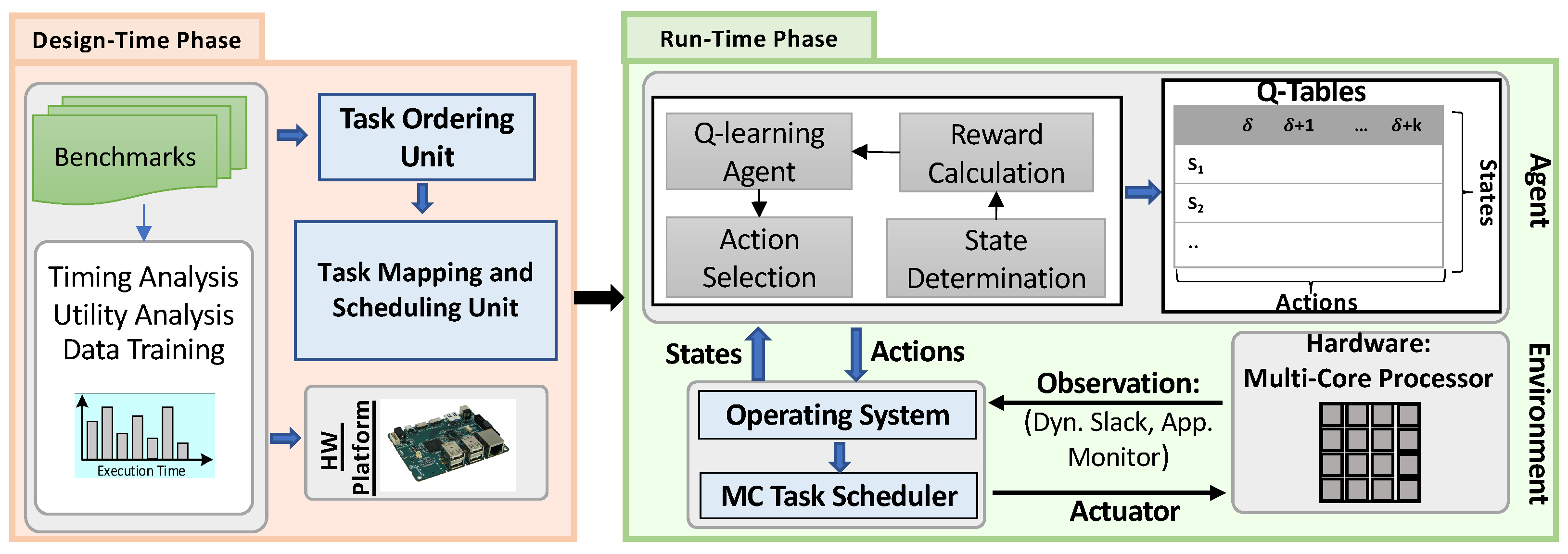
Figure 3.
Normalized QoS at run-time under different policies.

Figure 4.
Task schedulability by varying utilization bound (Comparing the proposed methods with Getting’15 [11], Ranjbar’20 [7], Liu’18 [9], Li’14 [12], and Huang’19 [8]).

Figure 5.
Normalized QoS at run-time by varying utilization bound (Comparing the proposed methods with Getting’15 [11], Ranjbar’20 [7], Liu’18 [9], Li’14 [12], and Huang’19 [8]).

Figure 6.
Normalized deadline miss rate at run-time when varying low-to-high WCET ratio (Comparing the proposed methods with Getting’15 [11], Ranjbar’20 [7], Liu’18 [9], Li’14 [12], and Huang’19 [8]).

Figure 7.
Normalized unused free dynamic slack at run-time when varying low-to-high WCET ratio (Comparing the proposed methods with Getting’15 [11], Ranjbar’20 [7], Liu’18 [9], Li’14 [12], and Huang’19 [8]).

Figure 8.
Normalized deadline miss rate at run-time when varying task mixtures (Comparing the proposed methods with Getting’15 [11], Ranjbar’20 [7], Liu’18 [9], Li’14 [12], and Huang’19 [8]).

Figure 9.
Normalized unused free dynamic slack at run-time when varying task mixtures (Comparing the proposed methods with Getting’15 [11], Ranjbar’20 [7], Liu’18 [9], Li’14 [12], and Huang’19 [8]).

Figure 10.
Drop-rate increment percentage under the proposed approach by varying task mixtures.
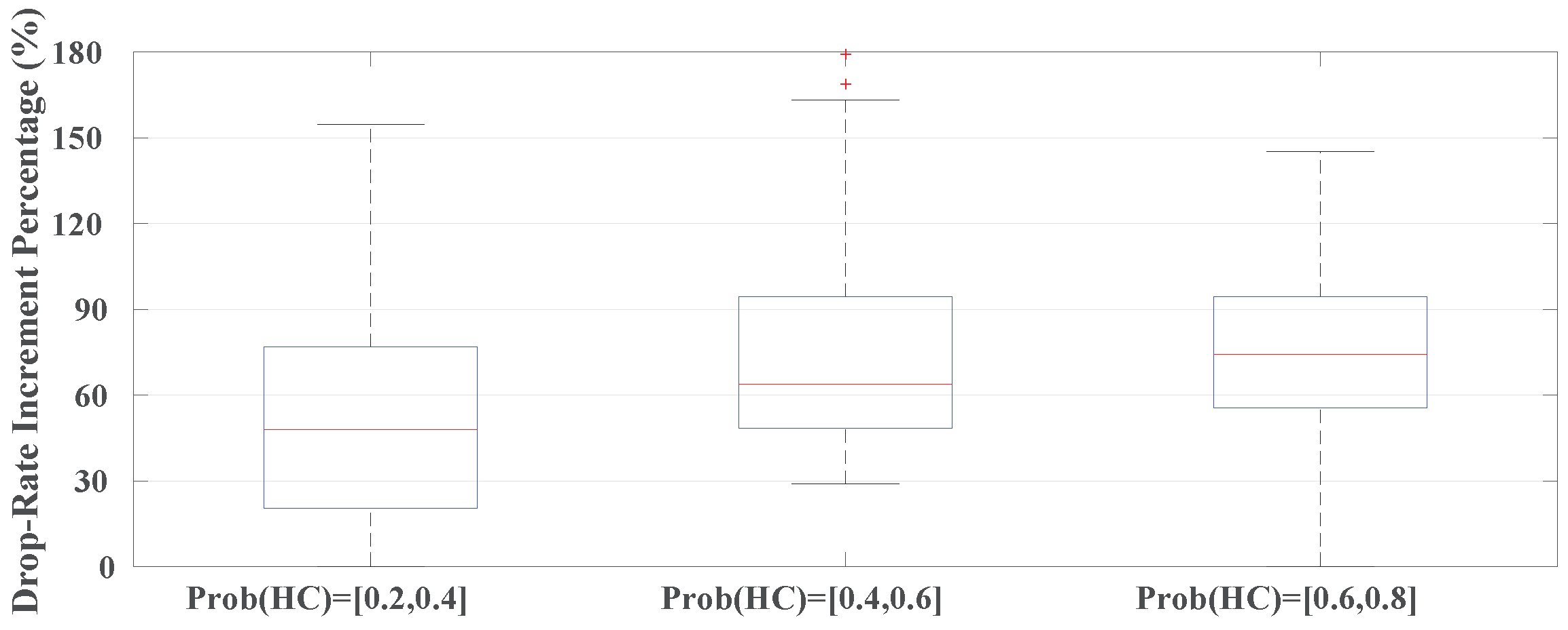

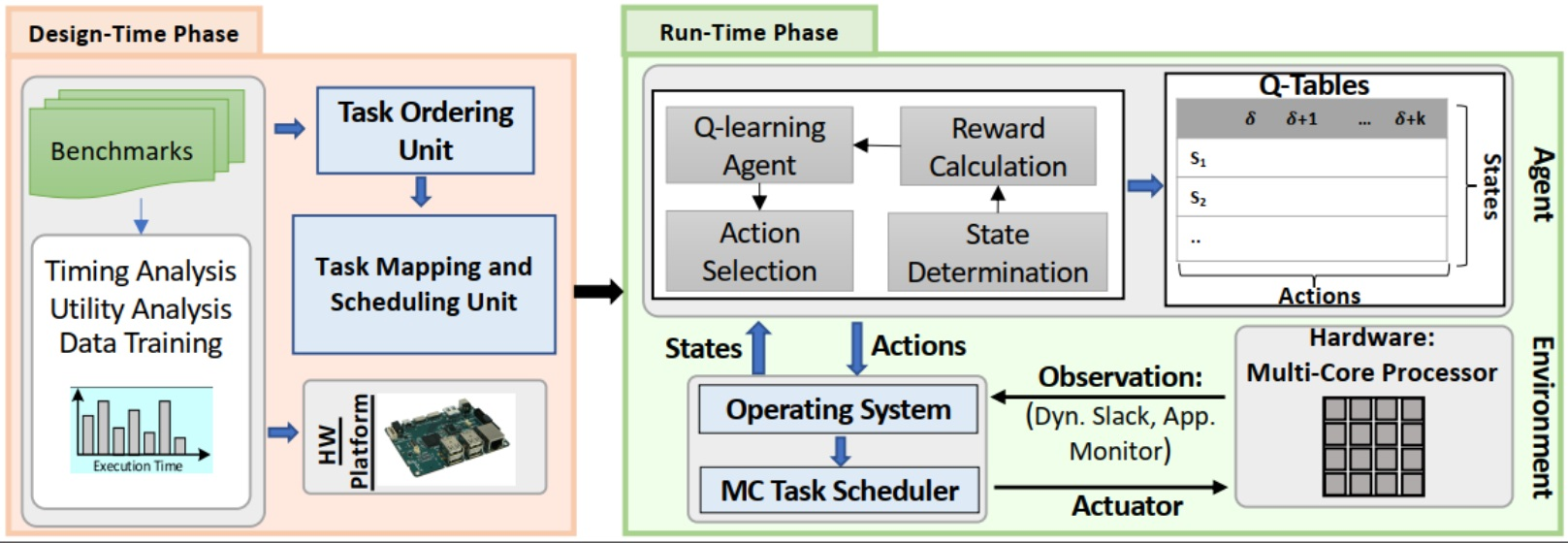
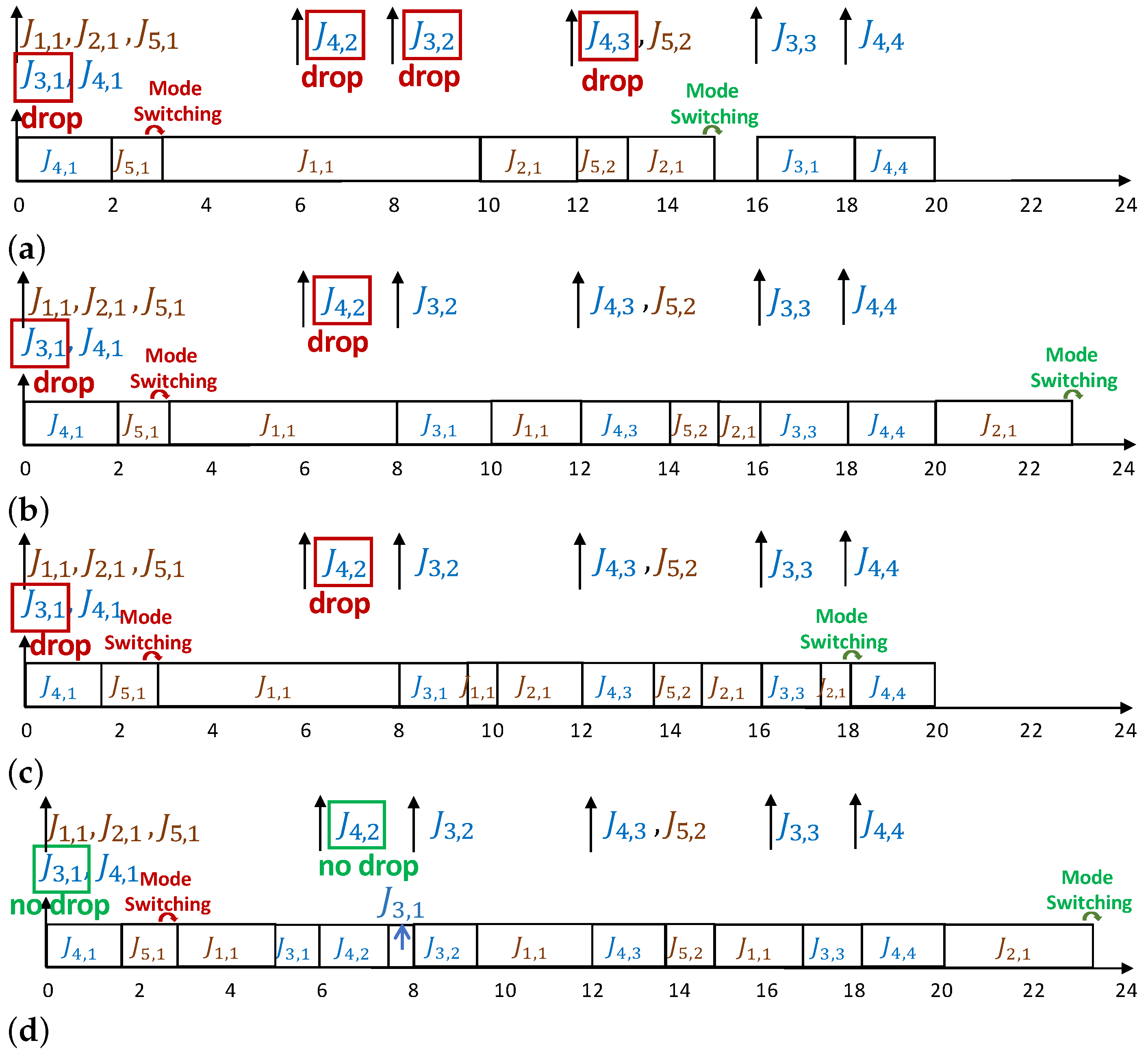
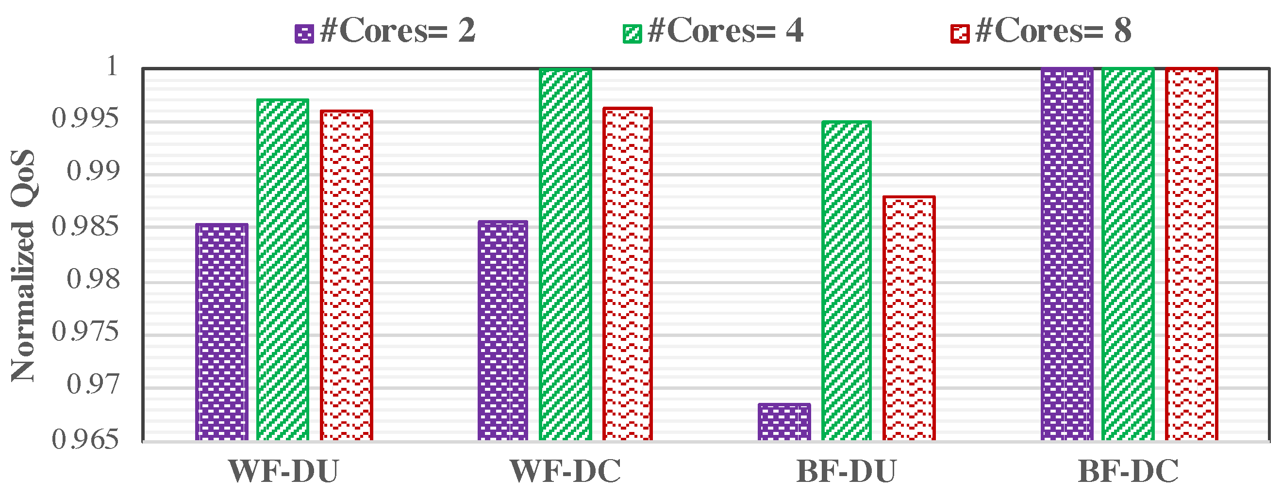
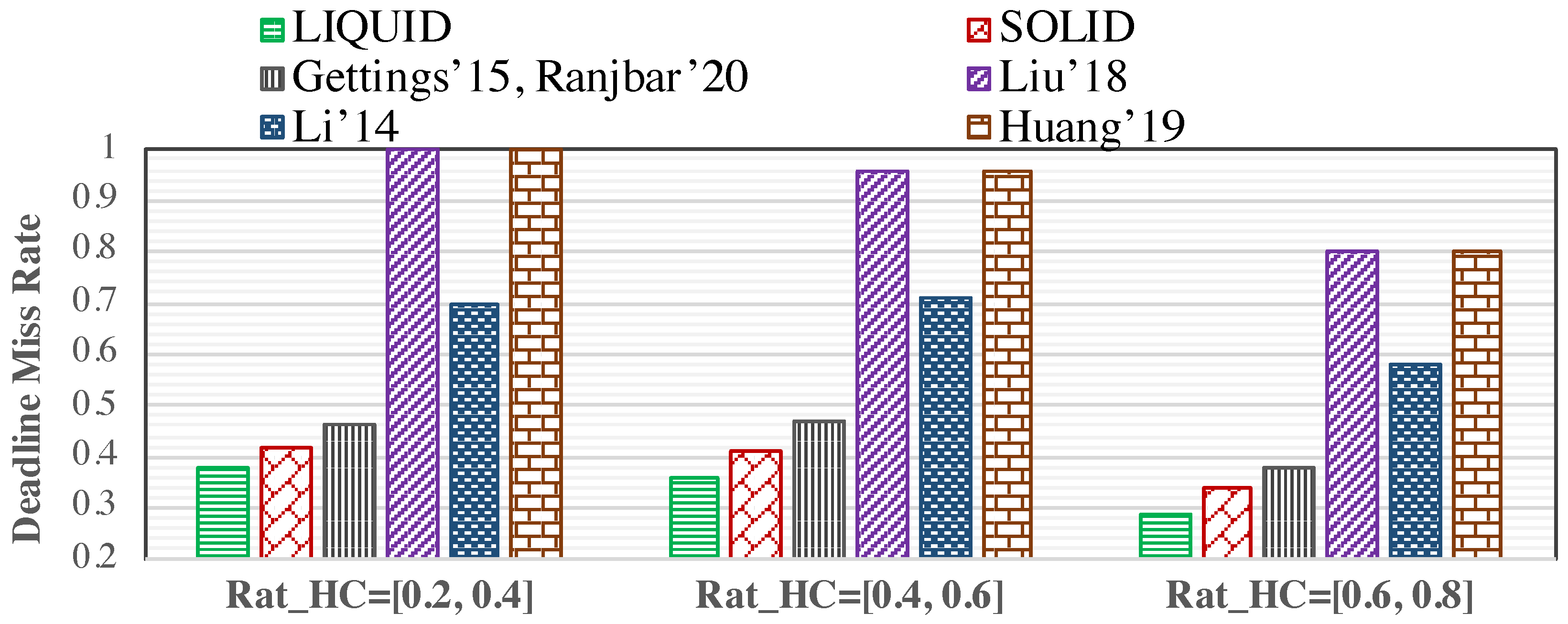
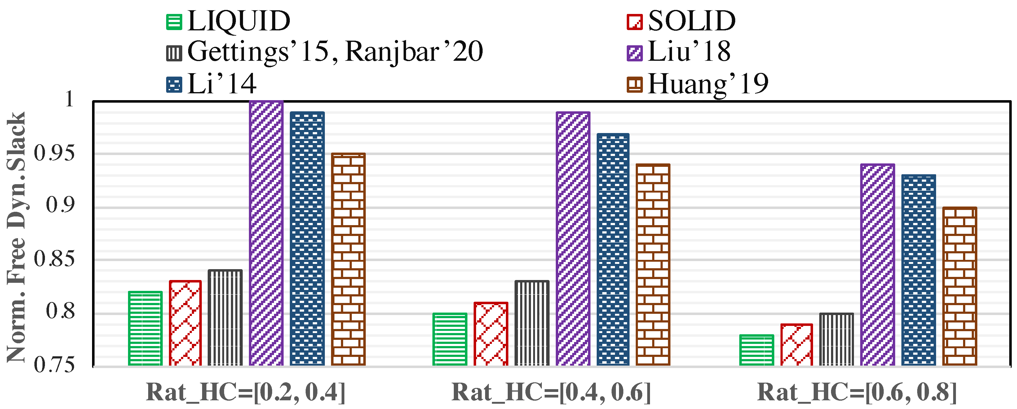
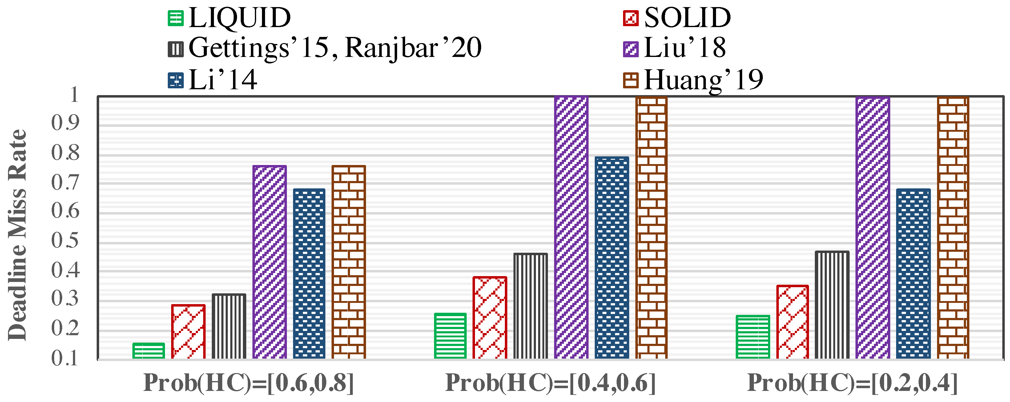
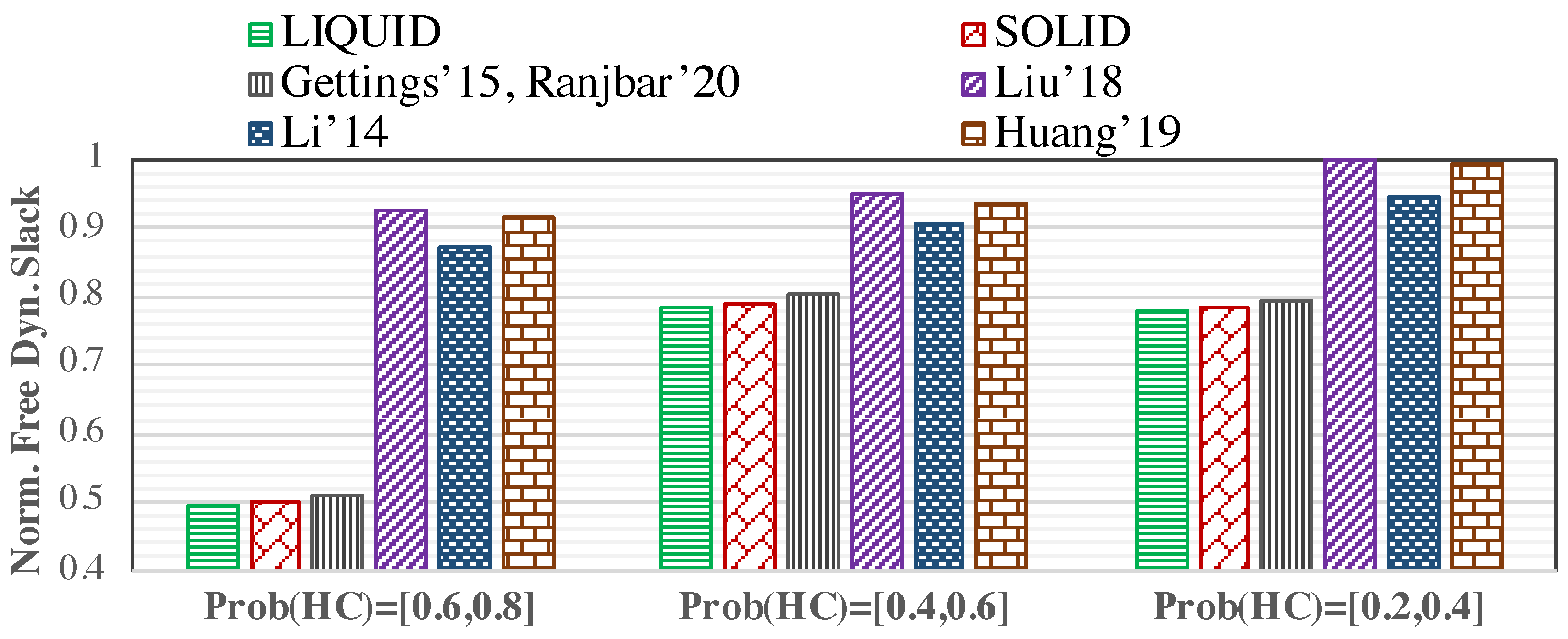
Table 1.
A brief overview on the state-of-the-art studies.
| # | S/M-Core | MC Tasks | Run-/Design-Time | QoS Opt. | Use of ML | |
|---|---|---|---|---|---|---|
| 1 | Gettings’15 [11], Ranjbar’20a [7], Liu’18 [9] Guo’18 [5], Ranjbar’21 [13] | S-Core | ✓ | Design-Time | offline | None |
| 2 | Ramanathan’18 [14], Pathan’17 [15], Pathan’18 [16] | M-Core | ✓ | Design-Time | offline | None |
| 3 | Sigrist’15 [17] | M-Core | ✓ | Run-Time | None | None |
| 4 | Huang’19 [8], Lee’17 [4], Li’14 [12], Hu’16 [18], Bate’15 [19] | S/M-Core | ✓ | Run-Time | online | None |
| 5 | Li’09 [20], Eom’13 [21], Horstmann’19 [22] | M-Core | × | Run-Time | None | ✓ |
| 6 | Proposed Work | M-Core | ✓ | Run-Time | offline & online | ✓ |
Table 2.
A list of used notations in this article.
| Symbol | Description | Symbol | Description |
|---|---|---|---|
| Criticality level of task | Skip parameter of task | ||
| Optimistic WCET of task | Pessimistic WCET of task | ||
| Actual deadline of task | Virtual deadline of task | ||
| Period of task | Hyper-period of task set | ||
| A released job (j) of task | Finish Time of task | ||
| Number of all LC tasks | Number of executed LC tasks |
Table 3.
The mixed-criticality task set.
| Task Function | |||||||
|---|---|---|---|---|---|---|---|
| engine control | HI | 2 | 7 | 24 | 11 | ∞ | |
| collision avoidance | HI | 2 | 4 | 48 | 22 | ∞ | |
| video capturing and transferring | LO | 2 | 2 | 8 | - | 3 | |
| sensor data recording | LO | 2 | 2 | 6 | - | 4 | |
| navigation | HI | 0.8 | 1 | 12 | 6 | ∞ |
Table 4.
NDM and QoS of different methods at run-time for a real task set.
| Metrics | LIQUID | Gettings’15 [11], Ranjbar’20 [7] | Liu’18 [9] | Li’14 [12] | Huang’19 [8] |
|---|---|---|---|---|---|
| NDM | 0.009 | 0.010 | 1 | 0.341 | 0.999 |
| QoS | 99.67% | 96.92% | 64.33% | 87.83% | 64.36% |
Table 5.
The values of normalized deadline miss rate and unused free dynamic slack at run-time when varying WCET ratio, shown in Figure 6 and Figure 7). The first value is normalized deadline miss rate and the second is unused free dynamic slack in each cell.
| LIQUID | SOLID | Gettings’15 [11], Ranjbar’20 [7] | Liu’18 [9] | Li’14 [12] | Huang’19 [8] | |
|---|---|---|---|---|---|---|
| = [0.2,0.4] | 0.38, 0.82 | 0.42, 0.83 | 0.46, 0.84 | 1.00, 1.00 | 0.70, 0.99 | 1.00, 0.95 |
| = [0.4,0.6] | 0.36, 0.80 | 0.41, 0.81 | 0.47, 0.83 | 0.96, 0.99 | 0.71, 0.97 | 0.96, 0.94 |
| = [0.6,0.8] | 0.29, 0.78 | 0.34, 0.79 | 0.38, 0.80 | 0.80, 0.94 | 0.58, 0.93 | 0.80, 0.90 |
Table 6.
The values of normalized deadline miss rate and unused free dynamic slack at run-time when varying task mixtures, shown in Figure 8 and Figure 9). The first value is normalized deadline miss rate and the second is unused free dynamic slack in each cell.
| LIQUID | SOLID | Gettings’15 [11], Ranjbar’20 [7] | Liu’18 [9] | Li’14 [12] | Huang’19 [8] | |
|---|---|---|---|---|---|---|
| = [0.6,0.8] | 0.15, 0.49 | 0.29, 0.50 | 0.32, 0.51 | 0.76, 0.93 | 0.68, 0.87 | 0.76, 0.92 |
| = [0.4,0.6] | 0.25, 0.78 | 0.38, 079 | 0.46, 0.80 | 1.00, 0.95 | 0.79, 0.90 | 0.99, 0.94 |
| = [0.2,0.4] | 0.25, 0.78 | 0.35, 0.78 | 0.47, 0.79 | 0.99, 1.00 | 0.68, 0.95 | 0.99, 0.99 |
Publisher’s Note: MDPI stays neutral with regard to jurisdictional claims in published maps and institutional affiliations. |
© 2022 by the authors. Licensee MDPI, Basel, Switzerland. This article is an open access article distributed under the terms and conditions of the Creative Commons Attribution (CC BY) license (https://creativecommons.org/licenses/by/4.0/).
Share and Cite
MDPI and ACS Style
Ranjbar, B.; Alikhani, H.; Safaei, B.; Ejlali, A.; Kumar, A. Learning-Oriented QoS- and Drop-Aware Task Scheduling for Mixed-Criticality Systems. Computers 2022, 11, 101. https://doi.org/10.3390/computers11070101
AMA Style
Ranjbar B, Alikhani H, Safaei B, Ejlali A, Kumar A. Learning-Oriented QoS- and Drop-Aware Task Scheduling for Mixed-Criticality Systems. Computers. 2022; 11(7):101. https://doi.org/10.3390/computers11070101
Chicago/Turabian StyleRanjbar, Behnaz, Hamidreza Alikhani, Bardia Safaei, Alireza Ejlali, and Akash Kumar. 2022. "Learning-Oriented QoS- and Drop-Aware Task Scheduling for Mixed-Criticality Systems" Computers 11, no. 7: 101. https://doi.org/10.3390/computers11070101
Note that from the first issue of 2016, this journal uses article numbers instead of page numbers. See further details here.