Non-Intrusive Load Monitoring Applied to AC Railways

Abstract

Non-intrusive load monitoring takes place in residential and industrial contexts to disaggregate and identify loads connected to a distribution grid. This work studies the applicability and effectiveness for AC railways, considering the highly dynamic behavior of rolling stock as an electric load, immersed in varying contexts of moving loads. Both voltage–current diagrams and harmonic spectra were considered for identification and extraction of features relevant to classification and clustering. Principal components were extracted, approaching the problem using principal component analysis (PCA) and partial least square regression (PLSR). Clustering methods were then discussed, verifying separability performance and applicability to the railway context, checking the performance by means of the balanced accuracy index. Based on more than one hundred measured spectra, PLSR has been confirmed with superior performance and lower complexity. Independent verification based on dispersion and correlation were used to spot relevant spectrum components to use as clustering features and confirm the PLSR outcome.

1. Introduction

Non-intrusive load monitoring (NILM) is a process or a technique used to disaggregate and identify loads from global metering points, e.g., at the feeding point of an installation or facility, transferring the concept to electrified transportation, at the traction power station (TPS). NILM is non-intrusive; namely, it does not use physical sensors at individual loads, relying on load signature recognition amid the power flow of the whole pool of connected loads. Load signatures are based on metrics that characterize load operating conditions, time patterns (if any), power absorption profiles, etc. NILM can effectively support network diagnostics, status monitoring, load management, power demand forecasting, and profiling [1,2,3].

NILM is based on a variety of techniques [4], which have proven to be effective at various degrees in a domestic context [5,6]; they are then considered for extensions to completely different applications, electrified railways, exploring the most promising signal features. The analysis is extended to both time- and frequency-domain data, considering voltage and current waveforms, instantaneous power, power trajectory, harmonic components, and harmonic quantities.

Electrified transportation systems, exemplified in this work by AC railways, feature highly dynamic moving loads entering and exiting supply sections, causing intermittent power absorption from a specific TPS [7]. In addition, the operation is characterized by power quality (PQ) issues [8,9,10,11,12] and complex harmonic signatures that depend on operating conditions [13,14].

As a first application to a railway system, the approach is based on feature extraction backed up by physical meaning. For this reason, wave shape (WS) features [2,15] are considered a starting point, having demonstrated significant discernibility in different home appliances. It should be acknowledged that discernibility was based years ago on substantially different power conversion architectures of the examined appliances, whereas for electrified rolling stock, the range is quite limited. Old AC locomotives were based on diode and possibly thyristor rectifiers [16], wheres modern ones are all equipped with four-quadrant converters (4QCs) [17,18,19]. Such loads differ from home appliances, making many WS features non-informative, as will be shown in this work (see Section 4.1).

For the same reason, the attention is directed to the thorough characterization of one or a few loads with known operating conditions, rather than starting from the identification of such loads in a more difficult context—that of measurements at TPS of the overall power flow of one supply section. When doing NILM on a power feeder, one element that brings additional information involves identifying the ’switch on and switch off’ events of the connected loads, possibly with their time patterns. In case of trains moving along the traction line, characteristic events involve the sudden changes of operating conditions (passing from standstill to acceleration, coasting, and braking [14]) and the passage under phase-separation points (seen as a switch off at one TPS and a new switch on at the adjacent one [13]). When measuring from a local pantograph perspective, other minor transients can occur, such as those caused by onboard load switching: many loads, such as pumps and compressors, have no power drive controls, and are switched on and off by direct connections, causing significant inrush currents and sudden reductions of the available line voltages; as for voltage sags in MV and LV distribution grids [20,21,22]: voltage sags are of much more relevance in industrial systems, whereas for electrified railways, such transients would not be clearly visible at the TPS measuring point. In general, they can be detected and assessed by a variety of methods [20,21,22] for quantification and triggering compensating systems [20], but are excluded from this analysis that is tailored to electrified AC railways, assuming locally stationary data following more slowly varying operating conditions.

Liang et al. [23] confirmed that active and reactive power plots are effective sets of features. In addition, high-order harmonics, instantaneous admittance (another way of quantifying the proportion between voltage and current spectra), instantaneous power, and eigenvalues can improve recognition capability.

NILM relies heavily on modern machine learning (ML) approaches [1,3,4,5], as well as more traditional techniques [2,15,24,25]. ML methods can be classified into supervised and unsupervised methods, using both deterministic and statistic approaches, whereas traditional techniques are based on more direct inspections of “electrical” quantities, such as voltage–current trajectories, active–reactive power plots, displacement factor discrimination, etc.

Unsupervised methods can proficiently be used in scenarios where labeling of operating states is not possible, allowing extraction of clusters from unsorted data. Basic clustering algorithms (such as k-means) rely on an assigned number of classes, making them de facto a partially supervised method. In addition, such methods perform well when data features are linearly separable. Conversely, evolved clustering methods, such as density-based spatial clustering of applications with noise (DBSCAN), provide indication of the optimal number of classes and can implement non-linear separation [26,27].

As a starting point, this work explores the basic characteristics of voltage and current waveforms of dynamic AC loads exemplified by rolling stock running on AC railways; this shows that commonly applied NILM techniques that perform well for home and office appliances are not effective for loads featuring much higher power levels and a uniformly applied wave-shape correction. It then evolves to the application of the discussed ML methods, focusing on the extraction of relevant features in the time or frequency spectrum domains, which allow effective clustering of the various operating conditions, separating components of external origins. The paper is structured into a preliminary description of AC railways (Section 2) and of classification and machine learning (Section 3). Section 4 presents the applications of such methods, distinguishing methods applicable to time domain waveforms and to spectral components for voltage, current, and power terms, in as many subsections. Section 5 discusses and summarizes the findings, leaving space to outline further developments and promising directions of research.

2. AC Railway System and Electrical Quantities

AC railways are peculiar electrical systems if compared to three-phase industrial networks: they are single-phase operated, use medium voltage (MV) levels, with an extension for each supply section of tens of km (up to about one hundred); the loads (i.e., rolling stock) move and have highly dynamic profiles, passing from standstill to tractioning, cruising, and braking. The traction line feeds power to such distributed loads by means of TPSs. AC railway systems in use today are mostly operated at 25 kV 50/60 Hz and 15 kV 16.7 Hz (for central Europe), yet with different supply schemes and different arrangements of supply sections. The supply traction line undergoes resonance phenomena at fairly low frequencies, possibly amplifying the distortion caused by the trains [28].

Assessments of rolling stock distortions are carried out for several reasons: traditionally, compliance to limits of emission to prevent interference to signalling [29,30], and in general, excessive induction [31,32]; more recently, attention has been placed on power quality with respect to the rest of the network [33], to resonance triggering and consequential overvoltages [28,34,35]. Finally, distortion has implications for power and energy consumption [36,37,38]; this is gathering more attention, i.e., in order to improve the energy efficiency of electrified transportation systems [39] in a sustainability perspective.

Rolling stock from different operators and manufacturers traveling over the line will have different emission patterns and distortion behaviors while changing the operating conditions.

There has been progress in power conversion, i.e., providing faster and more efficient converters, with more complex patterns of emission and distortion occurring over wider frequency intervals [17,18,19]. At the same time, electric transportation is reducing headway, necessitating faster dynamics and resulting in trains more densely arranged along the railway lines [40]. The harmonic spectrum of a vehicle in a real scenario features components of internal and external origins, the latter caused by the superposition of the terms of interacting rolling stock under a significant phase rotation depending on the relative position [41].

To study the problem and track distortion contribution, as well as identify loads by their distortion signatures, relevant power quantities must be defined first: the IEEE Std. 1459 [42] expresses voltage and current as vectors of harmonic components with a fundamental pulsation $\omega$,

$$\begin{array}{cc}\hfill v\left(t\right)& =V_0+\sqrt{2}\sum _{h=1}^{\infty }{V}_{h}sin(h\omega t+{\alpha }_h)\hfill \\ \hfill i\left(t\right)& =I_0+\sqrt{2}\sum _{h=1}^{\infty }{I}_{h}sin(h\omega t+{\beta }_h)\hfill \end{array}$$

(1)

where $V_h$ and $I_h$ are the amplitudes and ${\alpha }_h$ and ${\beta }_h$ the phases of order h.

Active and nonactive power terms may be defined, as known, with nonactive power further separated in reactive and distortion power:

$$p_a\left(t\right)=\sum _{h=1}^{\infty }{V}_h{I}_{h}cos{\theta }_h\left[1-cos(2h\omega t-2{\alpha }_h)\right]$$

(2)

$$p_q\left(t\right)=\sum _{h=1}^{\infty }{V}_h{I}_{h}sin{\theta }_h\left[1-sin(2h\omega t-2{\alpha }_h)\right]$$

(3)

$$p_d\left(t\right)=2\sum _{m=1}^{\infty }\sum _{n\ne m}^{\infty }{V}_m{I}_{n}sin(m\omega t-{\alpha }_m)sin(n\omega t-{\beta }_n)$$

(4)

These expressions lend themselves to recognise and classify fundamental and harmonic active power $P_1$ and $P_h$, fundamental and harmonic reactive power $Q_1$ and $Q_h$, and distortion power $D_h$, as commented in [14,43].

It should be noted that active and nonactive power terms are shown in (2), (3) and (4) as time domain functions, leading one to think that they may be exploited to plot loci similar to VI diagrams, providing an alternative. Such expressions in reality are defined, starting from $V_h$ and $I_h$, which are determined only on a cycle-wide basis, i.e., by the Fourier analysis. A valid approach in this respect, instead, is the instantaneous power theory and the use of “homo” integral and derivatives of voltage and current waveforms [44]. The present work is not complemented by this approach, as it would open the door to a large amount of interpretation of the resulting PQ trajectories that are much more complex than VI diagrams and are currently being developed.

In the fields of harmonic analysis and harmonic source identification, several approaches have been proposed based on classical manipulations of harmonic active power $P_h$ (tracking sign and intensity), distortion power $D_h$, and total nonactive power (or Fryze’s power). Except for harmonic active power, all other indices are collective and measure distortion as a whole, hinting at the origin based on small variations around reference values [43]. Changes of distortion patterns for varying operating conditions would be diluted and possibly go unnoticed if only collective indices were considered.

From this, there is a need to explore a fine-grain identification, down to the details of the single components of the harmonic power vectors if needed, but able to offer a synthetic representation without the burden of retaining all of the harmonic vectors. In other words, the expert examining patterns of power harmonic spectra could come out having selected a list of quantities with a strong relation to physical meaning, such as $P_h$ and $D_h$, possibly weighted on selected frequency bands. An example of selected harmonics related to the operation of (’own’ and extraneous) power conversion can be found in [14]. Traditional classification methods of the supervised type select an oversized pool of features in the data space and then subject these features to analyses aimed at identifying the most significant ones, using, e.g., principal component analysis (PCA), retaining entire spectra as autovectors, or partial least squares regression (PLSR), spotting out spectral components. Such features are then fed to clustering algorithms that exploit concepts of density or distance, to separate alike groups of data points.

The approach oriented to the component selection is well applicable to other scenarios, where sources and their operating conditions can be distinguished by spectral signatures (specific combinations of spectral components), as is the case of charging electric vehicles from different manufacturers, and possibly in different state-of-charge conditions [45].

Such methods are discussed in the next section.

3. Signal Features and Clustering

Signal features are considered in a broad sense, from time domain to frequency domain characteristics and quantities.

Time domain waveforms characteristics are often used for NILM involving home appliances, where there is a variety of front-end converters and conversion principles, whereas in large-power transportation applications there is some uniformity of architectures.

Frequency domain characterization is typically approached based on engineering judgment, supported by mathematical properties, such as correlation between components of different operating conditions and different rolling stocks, as discussed with some examples in [14]. The purpose is to identify frequency bins that are coherent for the same operating conditions (providing a compact feature that can be easily clustered) and show a significant diversity, or incoherence, when picked up from different operating conditions, or different rolling stocks.

3.1. Signal Features and Quantities

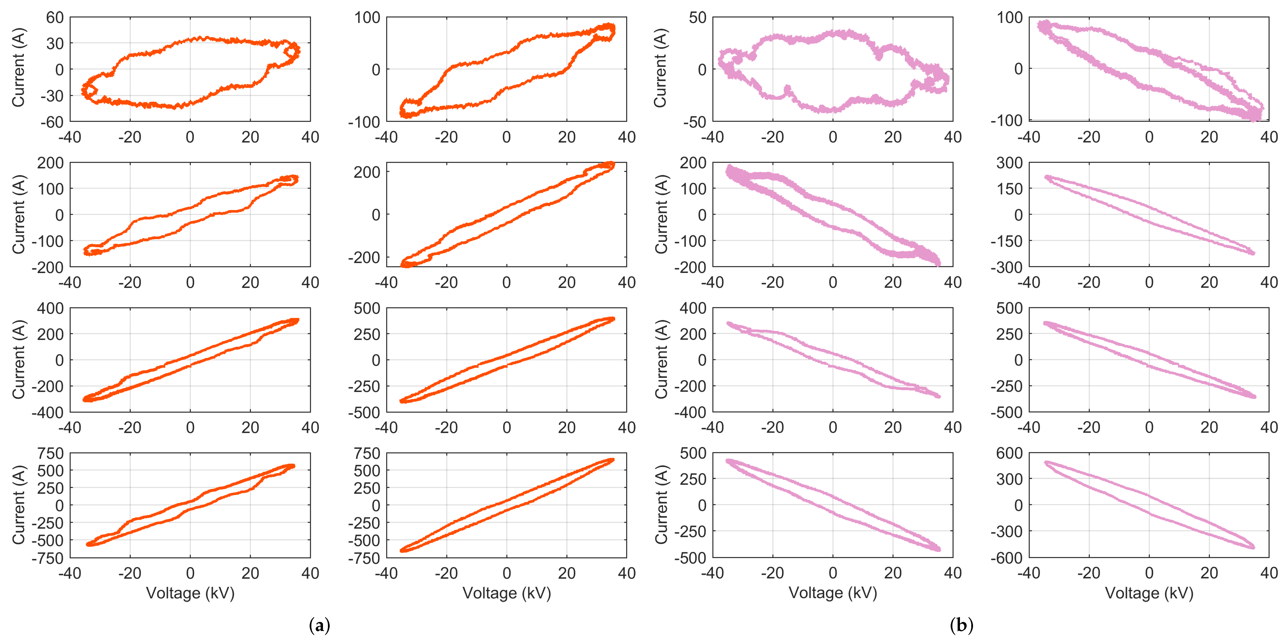
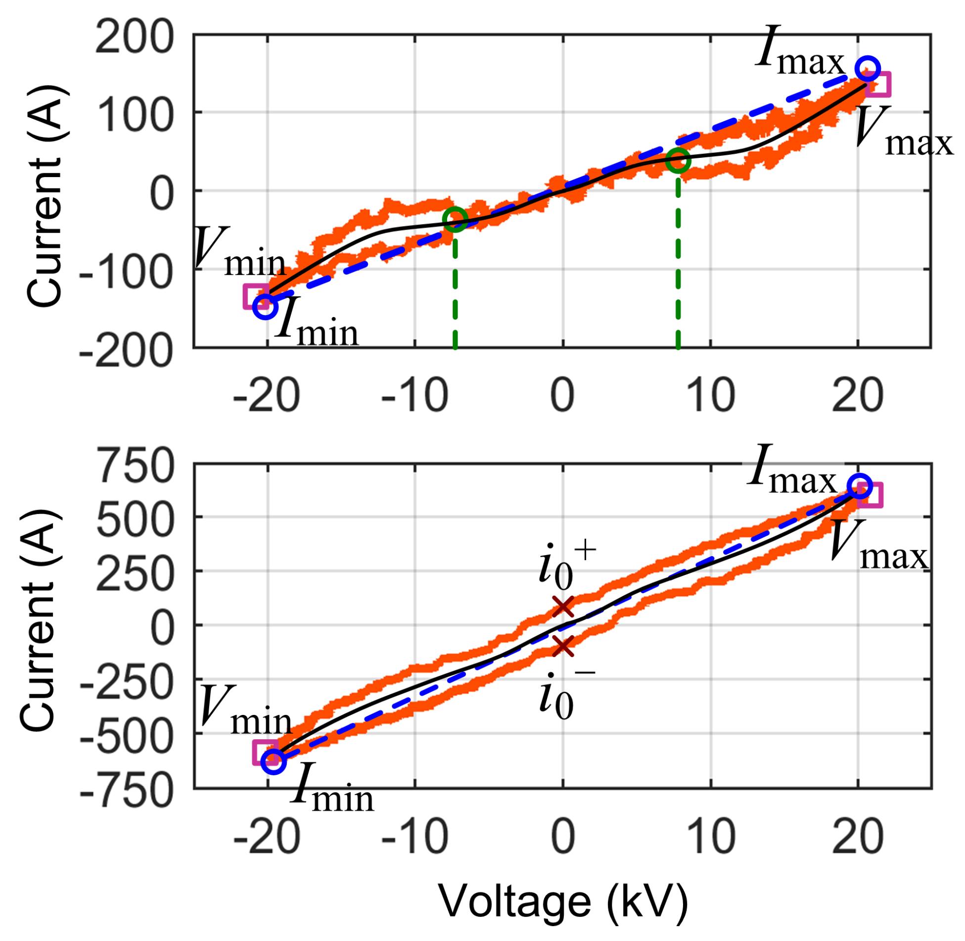
A wide range of features and index quantities can be extracted from rolling stock voltages and current recordings in time domain (waveforms) and from frequency domain spectra. Many of such quantities are common to industrial PQ; they were briefly reviewed in the previous section. In particular, when evaluated against a longer time horizon, they provide insight into the behavior of the source of distortion, especially regarding operating conditions [13,43].

Regarding the use of such indices for classification purposes, $P_h$ preserves information on the source down to a single component, whereas nonactive power terms are collective, with less interpretable behaviors. In addition, it could be observed that they have often been used without preserving their physical meanings, such as when reactive power terms are simply summed arithmetically rather than in quadrature [23].

Time domain waveforms, when suitably represented, provide a different type of information, as discussed below.

3.1.1. VI Diagrams

Lissajous diagrams were much exploited when the oscilloscope display was the only processing available, or nearly so. The most straightforward implementation is plotting $i\left(t\right)$ against $v\left(t\right)$, providing what is called instantaneous or time domain admittance y, which takes the form of closed curves with a periodically deformed elliptic path (periodic deformation is caused by harmonics). They are a significant source of information, regarding emission characteristics and spotting the differences between different loads.

A basic study may be carried out of the main plot characteristics, as discussed in [2], where they are identified as “wave-shape features” (although they are the features of a trajectory in the v-i plane, namely admittance):

• Loop direction of the VI locus, where the clockwise direction indicates capacitive behavior (which is quite uncommon in railways, being almost prohibited by the EN 50388 [46]), but also regenerative braking; the sign of current entering or exiting the pantograph provides clarification.
• Maximum and minimum points for the current (to compare with the total rms current $I_{\mathrm{rms}}$) and voltage (less significant, as it depends on the line supply condition, rather than the rolling stock itself); the slope $\psi$ of the line joining the current extreme points (opposed vertices of the curve) is commonly used as an indicator.
• Mean curve traversing the locus in the middle of the closed shape and joining the two vertices; the most meaningful index that can be extracted from it is its slope $\xi$ at some predetermined point, such as near the origin; in the following, the average slope in the first 30% of the x-axis voltage points will be used.
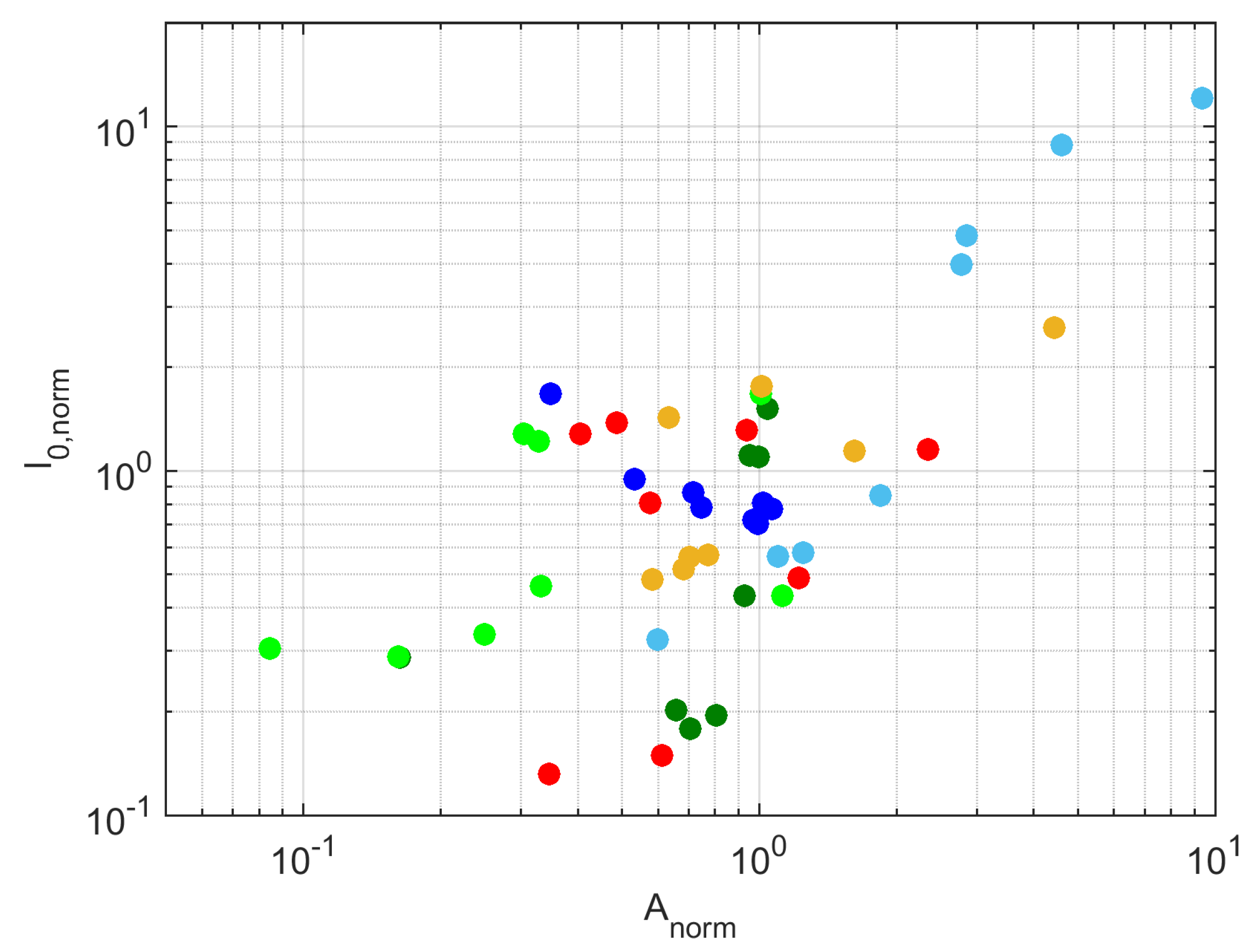
• Area A enclosed by the locus, measuring at the same time current intensity and loop aperture; this value should be normalized by the voltage intensity (to make the comparison of different systems possible, as well as different catenary voltage conditions) and by the current intensity (to compare different power absorption levels).
• Intersection points of the vertical i axis at $v=0$ ($i_0^{+}$ and $i_0^{-}$) and related span $i_0=i_0^{+}-i_0^{-}$.
• Presence of self intersections and their numbers $N_{\mathrm{inters}}$.

These features are demonstrated graphically in Figure 1, by taking two different shapes of the many VI diagrams of the Swiss system (see Section 4.1 for complete results).

Active and reactive power can be, in principle, plotted in a similar way, but the quantities in which we must focus on are not $P_h$ and $Q_h$ (defined and calculable only on a minimum time scale of one fundamental period and not suitable for the analysis of trajectory), impacting then on the time interval for definition of $p_a\left(t\right)$ and $p_q\left(t\right)$, or $p_d\left(t\right)$ (namely Equations (2), (3) and (4)), as observed in Section 2.

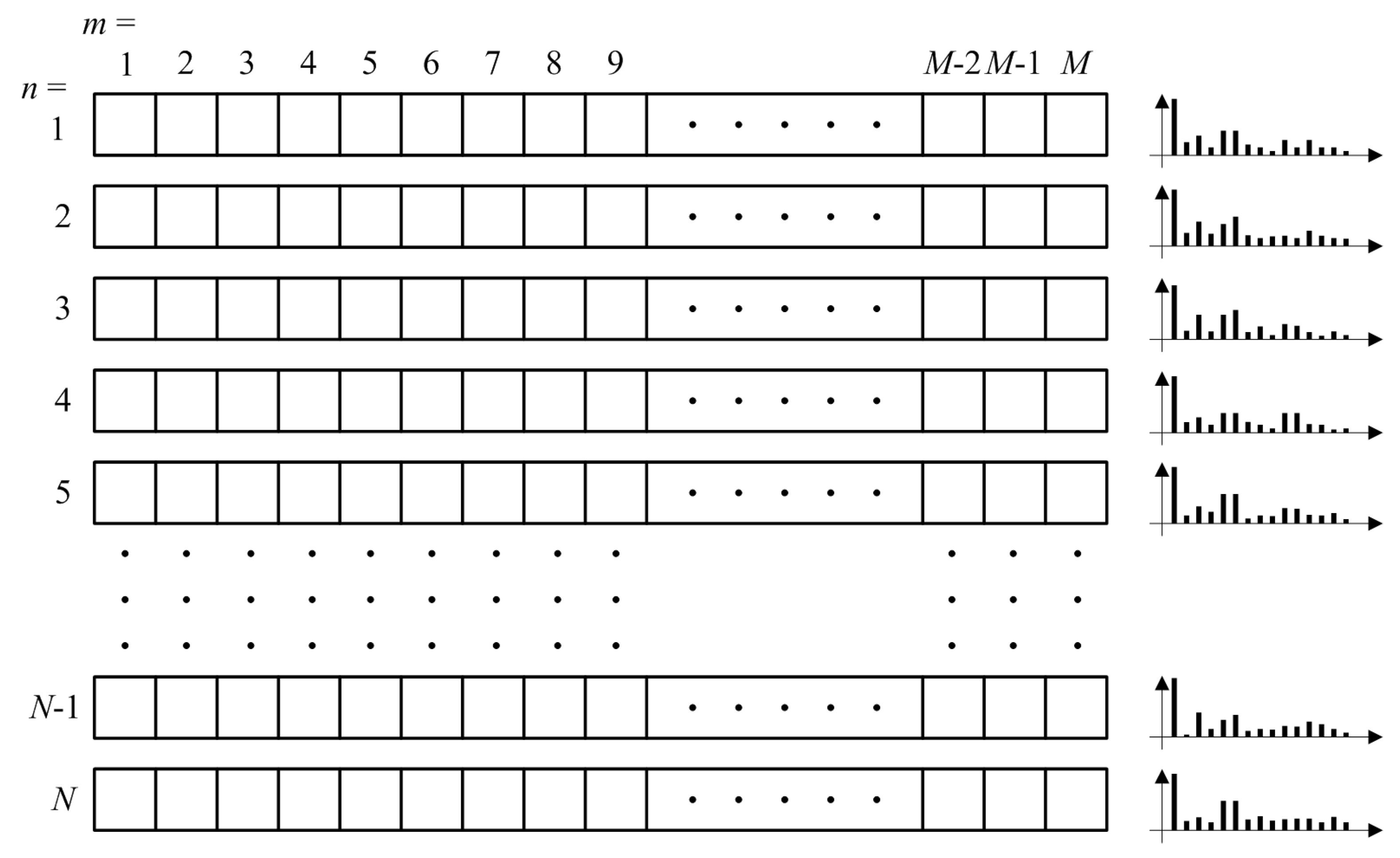
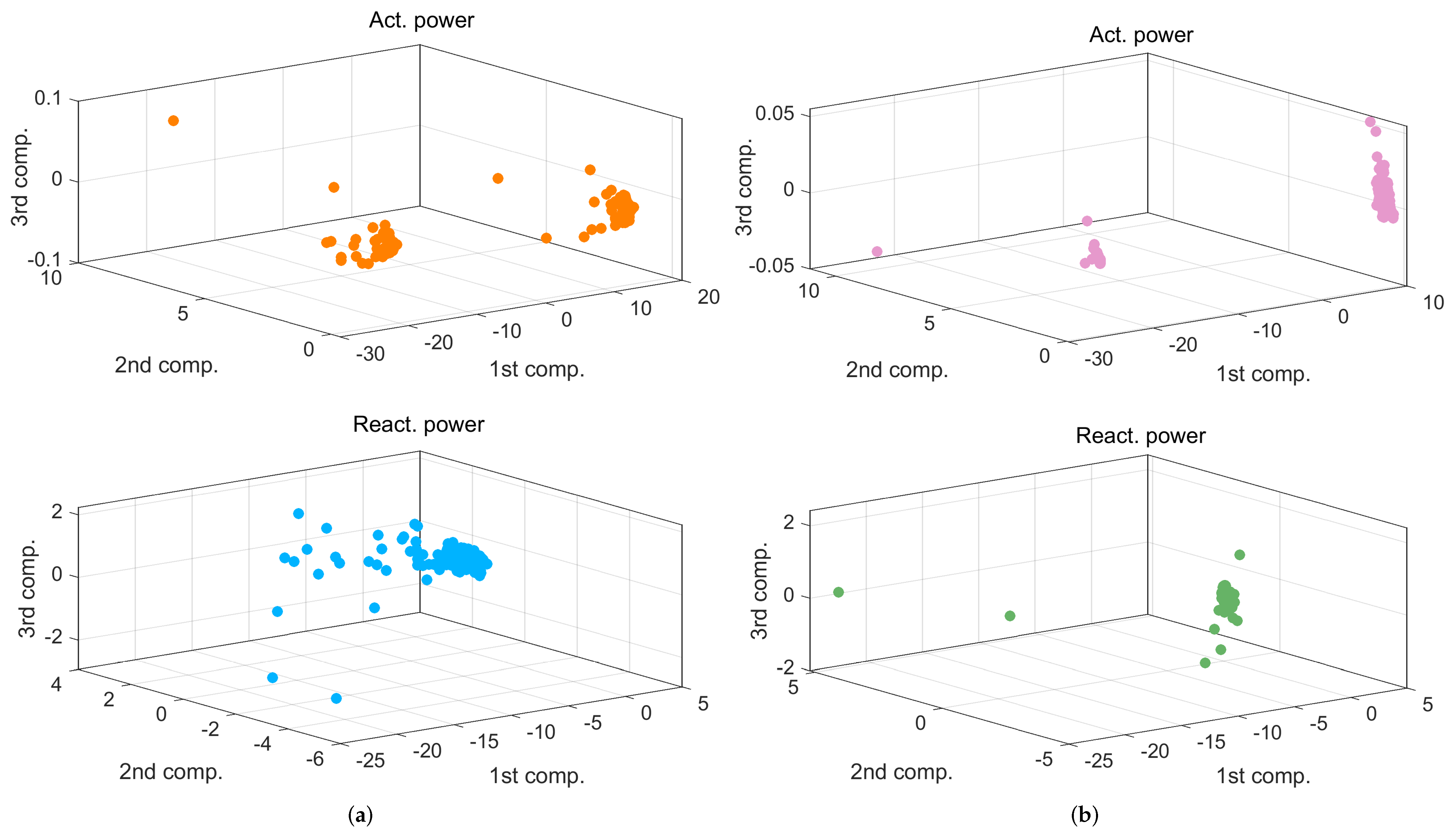
3.1.2. PCA and SVD Analysis

The application of some methods may require setting up data structures that at the current sampling rate for harmonic studies (e.g., 20 kHz to 50 kHz) become cumbersome and challenging to process. This is the case, for instance, with the SVD used in [23] to calculate signal eigenvalues. The instantaneous current $i\left(t\right)$ or power $p\left(t\right)$ waveform was split in cycle-long segments and rearranged in matrix form. Using the full sample rate for a low-frequency analysis would result in a 1 k × 1 k matrix spanning 20 s assuming a 50 Hz fundamental. Besides the fact that the 1000 cycle-long periods might be unavailable, operating conditions, as commonplace for railway applications, will certainly vary over the said time interval (resulting in overall non-stationarity).

A better form of analysis is pursued in Section 4, applying PCA (based on the SVD algorithm) and showing the independent components as measures of signal complexity and stationarity, when, for given operating conditions (e.g., traction or braking), distortion is expected to be qualitatively similar. To this aim, data records are limited, e.g., to those spanning over some tens of seconds during tractioning or braking.

PCA is a well-founded technique that seeks a linear combination of the features of provided data with minimum variance; thus, achieving a compact data representation. Data are arranged as: $N\times M$$\mathbf{X}$ matrix containing M columns of N collected observations each, with M different variables ${\mathbf{x}}_{\mathbf{m}}$ (column vectors of length N). In our problem, when PCA is applied to spectra, such variables coincide with the spectrum frequency bins. Such an arrangement is depicted in Figure 2.

The sought linear combination can be written as a vector of coefficient $\mathbf{a}$ that selects the desired (up to M, with $M\le N$) components of $\mathbf{X}$. Writing this as $\mathbf{X}\mathbf{a}$, it turns out that the objective of maximizing the variance can be written as [47]:

$$\mathrm{var}\left(\mathbf{Xa}\right)={\mathbf{a}}^{\prime }\mathbf{Xa}=\Lambda {\mathbf{a}}^{\prime }\mathbf{a}$$

(5)

where $\mathbf{S}$ is the sample covariance matrix associated with the data matrix $\mathbf{X}$ and ${}^{\prime }$ denotes transpose. With $\mathbf{a}$ being a unit-norm vector, the form with explicit eigenvalues $\Lambda$ holds.

The solution is an M-dimensional vector $\widehat{\mathbf{a}}$ that maximizes variance, but the most useful application in PCA involves keeping only those coefficients ($\widehat{\mathbf{a}}$ components) with the largest contribution to the variance (namely, corresponding to the largest eigenvalues), operating a reduction of dimensionality.

The obtained solution is an orthogonal base made of terms $\mathbf{X}\widehat{\mathbf{a}}$ that are called “principal components” (PCs). Once ordered from the largest to the smallest eigenvalue (as done ordinarily by PCA algorithms, such as for MATLAB), the subset of the first $M^{*}$ coefficients, contributing a fraction of the total variance of at least ${\gamma }^{*}$, constitutes a minimum set of PCs for the given level of significance ${\gamma }^{*}$. The total variance corresponds to the trace of $\mathbf{S}$, $\mathrm{tr}\left(\mathbf{S}\right)$, and each eigenvector ${\lambda }_m$ gives a contribution of ${\lambda }_m/\mathrm{tr}\left(\mathbf{S}\right)$. The fraction of energy brought in by the first $M^{*}$ eigenvalues is indicated by the quantity ${\gamma }^{*}$:

$${\gamma }^{*}=\sum _{m=1}^{M^{*}}\frac{{\lambda }_m}{\mathrm{tr}\left(\mathbf{S}\right)}$$

(6)

In general, mostly to avoid problems of ill-conditioning, the PCA algorithm is run using the centred version of the vector $\mathbf{X}$, obtained by subtracting for each component the mean value in the direction of observations, so along the index $n=1\dots N$.

3.1.3. Partial Least Squares Regression

Partial least squares regression (PLSR) has two major advantages with respect to PCA:

• It requires a smaller number of PCs to achieve the same quality of representation;
• PLSR includes the information of the second vector of responses y and it is more suitable to the wide class of classification problems.

In addition, it does not require that the number of observations N be larger than the number of variables M.

The general underlying structure of a PLSR problem can be described as follows. By analogy, with PCA, $\mathbf{T}$ is called the score matrix and $\mathbf{P}$ the loading matrix (in PLSR, the loadings are not orthogonal). $\mathbf{X}$ is decomposed as $\mathbf{T}{\mathbf{P}}^{\prime }$ and, likewise, an estimate of $\mathbf{y}$, $\widehat{\mathbf{y}}$, is decomposed into $\mathbf{T}\mathbf{B}{\mathbf{C}}^{\prime }$, where $\mathbf{B}$ is diagonal and takes the name of the regression weights matrix [48]. The looser representation of $\mathbf{Y}$, underlined by having used the word “estimate” is not worrisome in our context, as this term contains the labels that are comfortably assigned integer numbers and do not necessitate high numeric accuracy.

$$\begin{array}{cc}\hfill \mathbf{X}& =\mathbf{T}{\mathbf{P}}^{\prime }+\mathbf{E}\hfill \\ \hfill \mathbf{Y}& =\mathbf{T}\mathbf{B}{\mathbf{C}}^{\prime }+\mathbf{F}\hfill \end{array}$$

(7)

where $\mathbf{E}$ and $\mathbf{F}$ are two error terms.

Various PLS methods provide different estimates of $\mathbf{T}$, orthogonal or not, or can handle more complex responses, arranged as a whole matrix $\mathbf{Y}$ rather than a vector $\mathbf{y}$ (in the present case it simply contains the class labels).

The MATLAB implementation (function plsregress) uses the SIMPLS algorithm proposed in [49].

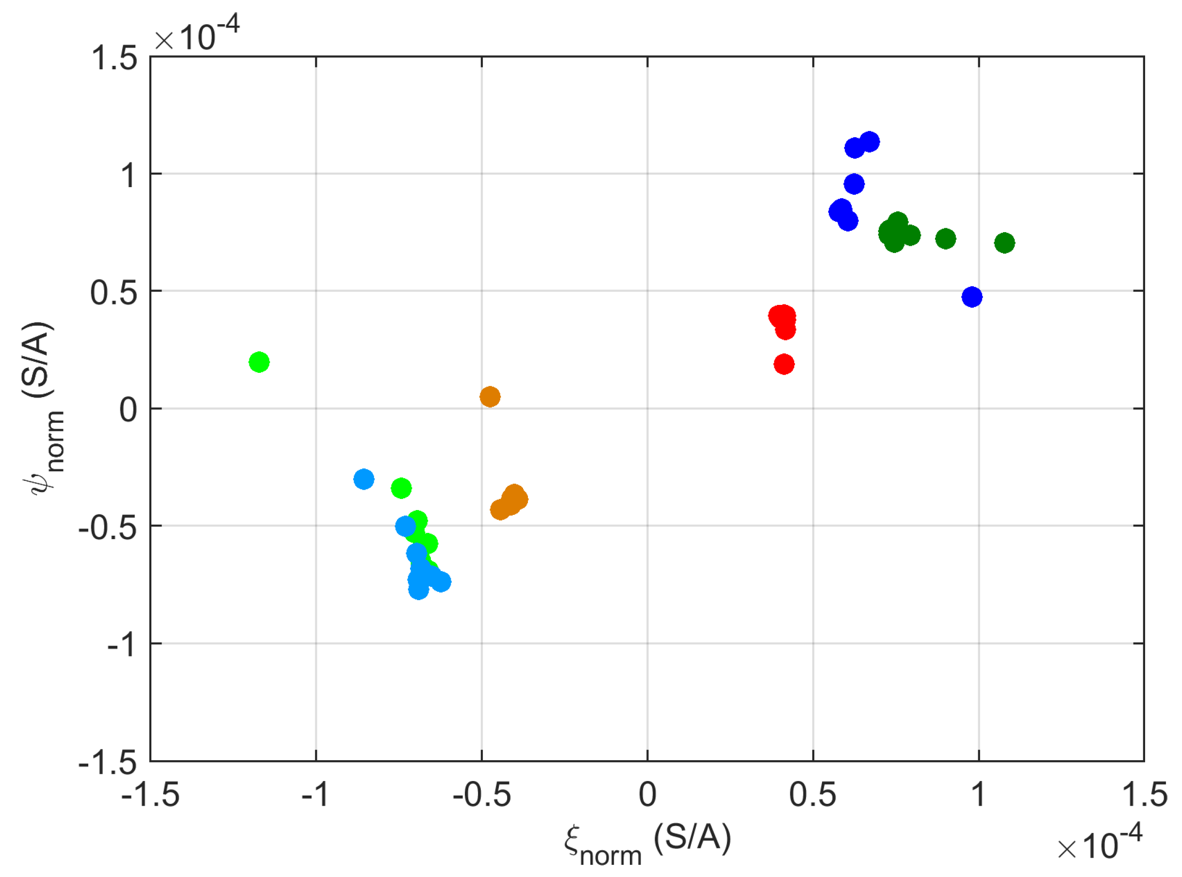
3.2. Cluster Analysis

The main objective of a classifier is to determine the label to assign to new unlabeled data, based on previously labeled data. In traditional classification, datasets are structured based on selected input attributes or features, and one output attribute (the class or label).

Cluster analysis, or clustering, is a form of machine learning of the unsupervised type, aimed at dividing provided data into clusters, which are then flagged separately. Clustering is based on the concept that data points belonging to the same group should have similar features.

From a general standpoint, clustering algorithms may be classified as:

• Density-based algorithms: grouping is carried out, identifying areas of high concentrations of points, separated by areas of low concentrations;
• Distribution-based algorithms: make some kind of assumption on the distribution of points around the supposed centroids, the probability reducing with distance indicates to which cluster a data point belongs;
• Centroid-based algorithms: similarly, the simple distance from centroids instructs how to separate data points;
• Hierarchical-based algorithms: it attempts to create a hierarchy of data by either an agglomerative approach (bottom-up, combining smaller clusters) or divisive approach (top-down, splitting into smaller clusters starting from one large cluster of all data).

To this aim clustering techniques are mostly based on the metric of distance between data items in a given space of representation. Data are grouped based on their perceived compactness, not only a short distance between points of the same cluster, but also a significant separation from neighbouring points of other clusters. Some clustering algorithms require to first specify the number of clusters inherent to the data; others may require that a minimum distance between data points is specified to consider them “connected”.

New data can be classified as belonging to one cluster or another, based on the said metric. Two main problems occur when dealing with feature-rich data showing high dimensionality:

• The predictive performance of a classifier decreases as the number of features increases, while keeping the number of training instances constant [50]; in other words, training should be augmented in terms of the number of instances, at least proportionally to the increase in the number of features;
• The metric based on distance tends to lose significance as dimensionality grows [51].

So, a fundamental objective for effectively operating clustering algorithms involves reducing dimensionality, by identifying the most relevant features, with care for compact representation.

3.2.1. K-Means

K-means is a centroid-type algorithm, based on a straightforward application of the concept of a higher density of data points to justify their belonging to a cluster. The algorithm aims to minimize the sample dispersion of data points within a cluster. Namely, the criterion to assign data points to a cluster involves the Euclidean distance from the current centroids; centroids are determined from the calculated means. At each iteration for the current partitioning of data points, means are calculated and assigned to the centroids. If the new mean values do not change from the previous iteration, the algorithm is stopped.

K-means has the limitation of fixing a priori the number of clusters, and since it iterates over all data points, it is not efficient with large datasets. The method also has difficulties in clustering non-convex or overlapping datasets. However, it could be considered a basic clustering method and it is a useful reference. It has been acknowledged that many other methods fix the number of clusters and it is a minor issue, possibly by attempting a few different choices and selecting the best one.

3.2.2. Density-Based Spatial Clustering of Applications with Noise

A significant improvement is represented by the density-based spatial clustering of applications with noise (DBSCAN) method, which has some important advantages:

• It does not fix the number of clusters a priori;
• It has the ability of separating outliers labeling them as “noisy points”, possibly reinserting them into a cluster during the process;
• It works effectively with non-convex data points.

However, there are two main drawbacks:

• Performance is impaired by data groups featuring varying density, as the distance threshold and minimum point required to form a cluster should be continuously adapted;
• It may face a similar problem for high-dimensional data, which is, in any case, alleviated by pre-processing data with feature extraction techniques, such as the autoencoder.

3.2.3. Mean Shift

Mean shift is another centroid-based iterative algorithm that assumes distribution of points around supposed centroids by taking a kernel function $F\left(\right)$ (usually Gaussian, with respect to distance, hinting that data points are dispersed because of noise or by a combination of random errors). Using $F\left(\right)$ as a weight function, the first assumed center is replaced by the calculated mean of the data points, falling into the cluster of the centroid; convergence occurs when the difference between the old center and the new calculated mean (called namely “mean shift”) is below a given threshold.

The selection of $K\left(\right)$ is critical, but a few geometries are available; in addition, there is no formal proof of convergence for increasing data dimensions. Similar to k-means, mean shift has difficulties in clustering non-convex or overlapping datasets.

3.2.4. Gaussian Mixture Model

K-means places regions of circular shapes to capture clusters and it performs poorly with oblong data clusters (where data spread differently along, e.g., orthogonal directions). The Gaussian mixture model (GMM) has more degrees of freedom, allowing to modulate the extension of the cluster region along each axis. In addition, GMM features a version with soft classification, assigning to data the probabilities of belonging to the given clusters.

The GMM algorithm deals with a set of Gaussian distributions of mean ${\mu }_k$ and dispersion ${\sigma }_k$, in numbers equal to the number of clusters K; for each distribution, there is also a fraction of data points belonging to it, called density ${\pi }_k$. The algorithm iteratively updates these parameters passing through three steps:

• During the estimation phase, the probability is calculated for each datum point, $x_i$, belonging to each cluster, given the distribution and the actually assigned point (number $n_k$ for each cluster):

  $$r_{i,k}=\frac{\mathrm{Pb}\{x_i\in k^{*}}{\}}\sum \mathrm{Pb}\{x_i\in \mathrm{other}\mathrm{than}{k}^{*}\}=\frac{{\pi }_{k^{*}}\mathcal{N}({\mu }_{k^{*}},{\sigma }_{k^{*}})}{{\sum }_{k\ne k^{*}}{\pi }_k\mathcal{N}({\mu }_k,{\sigma }_k)}$$

  (8)
• Data point $x_i$ is assigned to cluster k following the indication of the largest $r_{i,k}$ values;
• During the maximization phase, parameters are updated, calculating ${\pi }_k$ as the fraction of the number of data points effectively assigned to cluster k, and quantities updated as follows with similarity with mean shift for $\mu$ (referred to $k^{*}$, with $k^{*}=1\dots K$):

  $${\pi }_{k^{*}}=\frac{n_{k^{*}}}{{\sum }_{k=1,}^K{n}_k}{\mu }_{k^{*}}=\frac{1}{n_{k^{*}}}\sum _i{r}_{i,k^{*}}{x}_i{\sigma }_{k^{*}}=\frac{1}{n_{k^{*}}}\sum _i{r}_{i,k^{*}}{(x_i-{\mu }_{k^{*}})}^{\prime }(x_i-{\mu }_{k^{*}})$$

  (9)

We will see that GMM results in a poorer performance compared to k-means (Section 4.4), as if the additional information it deals with (dispersion) is in some way counterproductive for this specific problem.

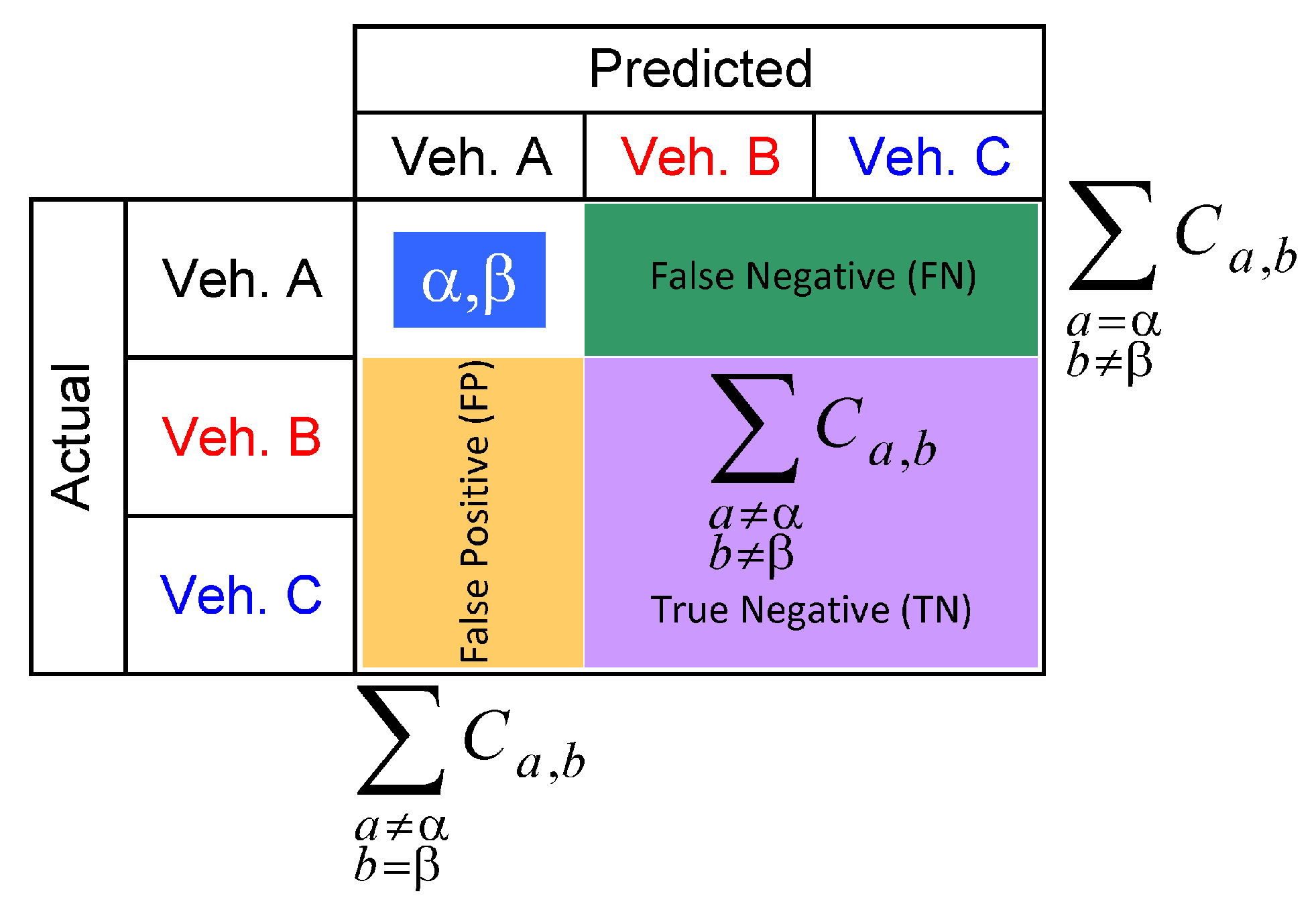
3.3. Verification of Performance

For demonstration and discussion of signal and spectrum features, it would be hard to find a formal quantification of performance, although criteria are followed to assess the effectiveness and relevance of a particular feature. Regarding classification and clustering, instead, performance is assessed using selected indices against a set of test signals.

In general, evaluating the performance of correct identification and separation is subject to different standpoints, depending on what is deemed more relevant: in the present situation, a balanced evaluation is carried out, similarly weighting all classification errors. Performance assessment is built around a set of cases representing $V=3$ vehicles (synonymous of locomotive or electric unit) and $O=2$ operating conditions (traction and braking).

The confusion matrix $\mathbf{C}$ summarizes the results of a classification problem by counting the number of correct and incorrect predictions for each class. A binary confusion matrix is such that results are classified with obvious meanings, such as true positive (TP), true negative (TN), false positive (FP) and false negative (FN). Then many indices of performances that are reviewed below can be straightforwardly applied. For multi-class problems, the binary structure is not immediate (see Figure 3) and binary indices seem to be inapplicable. In reality, selecting one particular case (indicated as $\alpha ,\beta$ for the TP case), the rest of $\mathbf{C}$ can be arranged to determine the remaining TN, FP, and FN. As alternatives, there are binary indices that may be applicable, straightforward, to multi-class scenarios.

$$TN=\sum _{\begin{array}{c}a\ne \alpha \\ b\ne \beta \end{array}}{C}_{a,b}FP=\sum _{\begin{array}{c}a\ne \alpha \\ b=\beta \end{array}}{C}_{a,b}FN=\sum _{\begin{array}{c}a=\alpha \\ b\ne \beta \end{array}}{C}_{a,b}$$

(10)

Of the entire set of conventionally-named positive cases for a given operating condition, o, for a given vehicle, v, indicated by $P={\displaystyle \sum _{b=1}^K}{C}_{\alpha b}$, the ratio of those truly classified as positive $TP=C_{\alpha \beta }$ defines the “hit ratio” (or “sensitivity”): $TP/P$. Symmetrically, the performance for a negative case is named “specificity” and expressed as $TN/N$.

The concept of minimizing $FP$ may reflect into “precision” $TP/(TP+FP)$ (if weighted against TPs) or “fall-out rate” $FP/N=FP/(FP+TN)$ (if considering FPs as negative cases leaked, or fallen out, into a positive classification).

Without leaning toward any particular case or scenario, the objective becomes the minimization of off-diagonal terms, which improves separation and reduces falling-out cases to a minimum.

An accurate and comprehensive measure of performance that will be used in the following is balanced accuracy (BA), which combines the correct classifications for both positive and negative cases (weighting TP and TN values),

$$BA=\frac{1}{2}\left(\frac{TP}{P}+\frac{TN}{N}\right)$$

(11)

and is applicable to multi-class scenarios:

$$BA=\frac{{\displaystyle \sum _{\begin{array}{c}a=1\\ a=b\end{array}}^K}{C}_{a,b}}{{\displaystyle \sum _{a,b=1}^K}{C}_{a,b}}$$

(12)

Other performance indices used, e.g., for medical diagnostics, tend to privilege conservatively efficacy on positive cases, such as the diagnostic odds ratio. For this reason, attention is focused on indices giving an overall metric of performance and that are easily applicable to multi-class scenarios.

4. Exemplification and Results of Classification

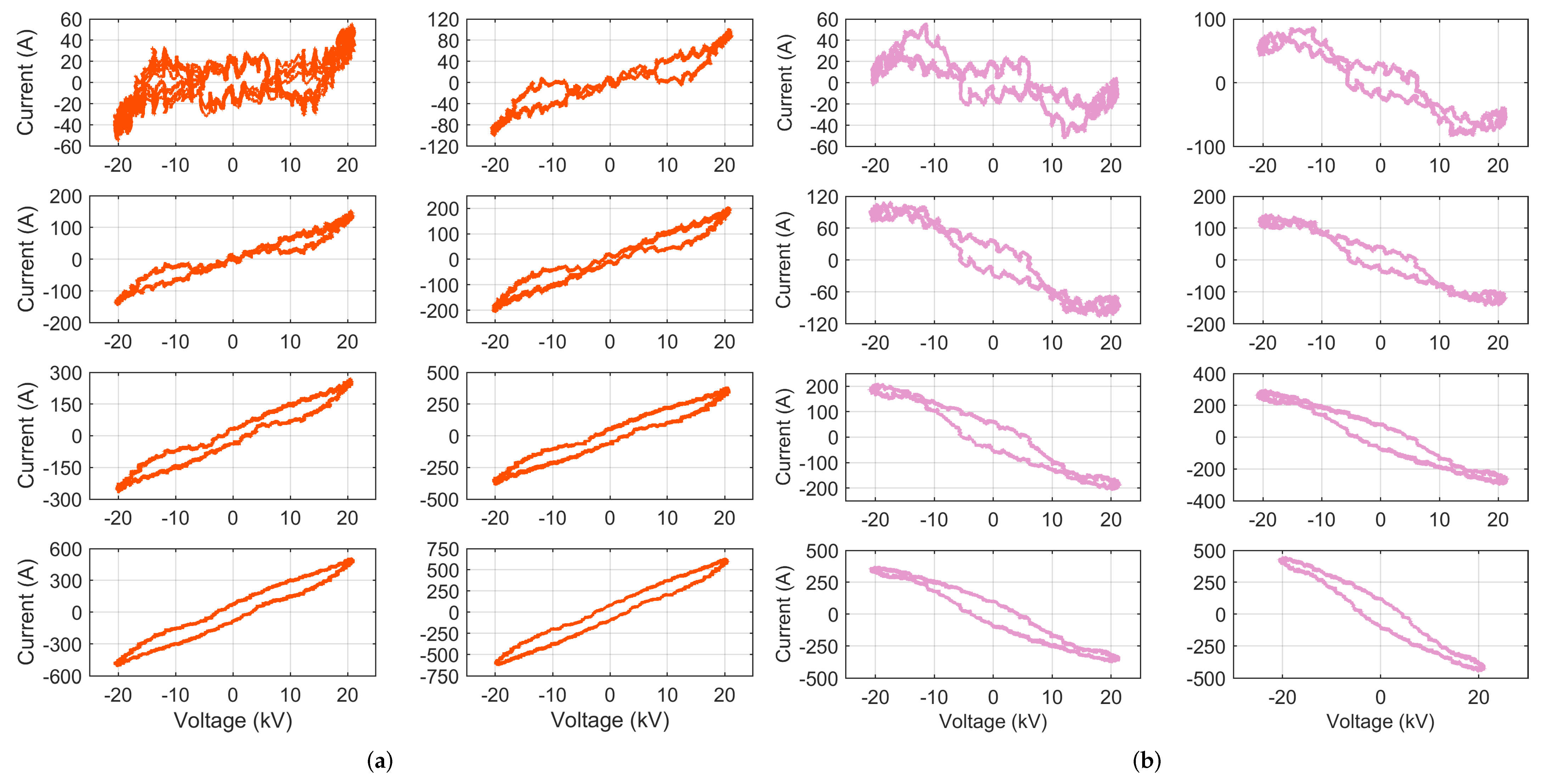
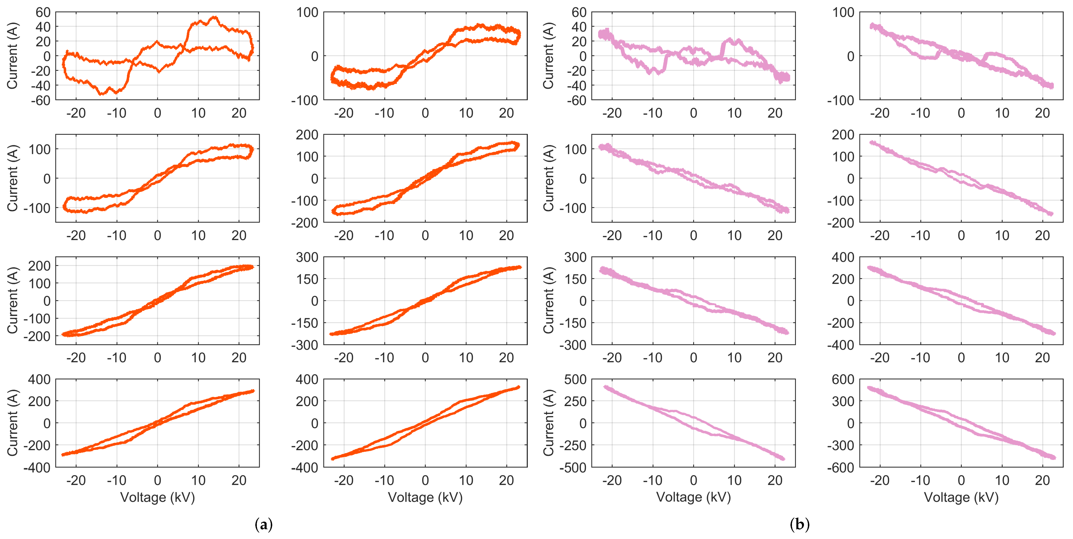
The previously discussed approaches to NILM and load classification are put in practice with data provided in a large dataset of pantograph electric quantities, tagged also for speed, total rms current, and operating conditions [52].

Data are processed by means of discrete Fourier transform (DFT) using a Hanning smoothing window. The use of smoothing windows is possible due to the synchronization of data in [52], aligned with zero-crossings. Measured data are provided for all three countries considered in this analysis (Switzerland, Germany, and France) in the form of short records of five fundamental cycles called “snippets” that allow both multi-cycle and sliding-window single-cycle DFT (namely short-time Fourier transform), the latter was used in this work to obtain average amplitude spectra, in attempt to reduce data variability.

The measuring system and setup are described in [53], including an estimate of its uncertainty, which is roughly in the order of 1–2% for the voltage and current channels. Such a system was installed in three different rolling stock items in the three respective countries collecting pantograph quantities (voltage and current) for several days, either in normal commercial service (Switzerland and France) or during special tests of acceleration and braking (Germany).

4.1. VI Diagrams

Lissajous diagrams are shown in the following for some selected current levels in tractioning and braking conditions for the three railway systems (Switzerland, Germany, and France, in Figure 4, Figure 5 and Figure 6, respectively). VI locus parameters are then summarised in

Table 1. VI diagram parameters for Switzerland (case numbering from 1 to 8, following Figure 4).

Case	Irms (A)	A (MVA)	Vmin (kV)	Vmax (kV)	Imin (A)	Imax (A)	$\mathit{\xi }$ (mS)	$\mathit{\psi }$ (mS)
Tra1	24.3	0.0593	21.10	−20.58	54.49	−54.65	2.62	1.72
Tra2	53.6	0.5680	21.18	−20.68	101.84	−100.02	4.82	3.87
Tra3	83.9	0.8287	21.10	−20.45	138.05	−138.36	6.65	6.18
Tra4	122.0	1.4746	20.93	−20.44	187.60	−188.12	9.08	8.65
Tra5	165.4	2.3639	20.89	−20.40	258.55	−258.08	12.51	13.14
Tra6	240.4	3.5886	21.03	−20.50	362.53	−369.02	17.61	18.30
Tra7	328.8	5.1505	20.88	−20.63	495.86	−497.66	23.93	24.83
Tra8	412.5	5.7500	20.61	−20.07	613.71	−610.52	30.09	30.55
Brk1	21.3	0.1114	21.21	−20.60	54.64	−49.79	−2.50	0.42
Brk2	52.5	0.4189	21.13	−20.72	85.70	−78.10	−3.90	−1.77
Brk3	72.9	0.7821	21.47	−20.90	108.38	−106.42	−5.07	−3.49
Brk4	96.2	1.0762	21.14	−20.77	141.41	−142.27	−6.76	−5.09
Brk5	144.1	2.2006	21.45	−21.10	204.76	−202.55	−9.57	−8.29
Brk6	202.4	3.2431	21.63	−21.03	295.41	−296.26	−13.87	−13.14
Brk7	262.8	3.8325	21.47	−20.94	368.65	−367.51	−17.36	−18.15
Brk8	311.8	4.6487	21.31	−20.82	443.19	−437.03	−20.90	−22.02

,

Table 2. VI diagram parameters for Germany (case numbering from 1 to 8, following Figure 5).

Case	Irms (A)	A (MVA)	Vmin (kV)	Vmax (kV)	Imin (A)	Imax (A)	$\mathit{\xi }$ (mS)	$\mathit{\psi }$ (mS)
Tra1	23.3	0.8209	23.44	−23.27	53.49	−53.06	2.28	1.11
Tra2	44.8	0.8197	23.23	−23.03	68.14	−70.73	3.00	5.09
Tra3	79.0	1.1113	23.23	−23.06	113.60	−115.47	4.95	8.76
Tra4	116.9	1.0105	22.45	−22.98	165.39	−165.60	7.29	11.18
Tra5	148.6	0.7708	23.07	−22.86	197.81	−202.32	8.71	12.61
Tra6	174.6	1.0620	23.26	−23.04	234.60	−232.98	10.10	14.64
Tra7	214.2	1.9642	23.41	−23.19	291.60	−293.99	12.57	18.04
Tra8	238.7	1.7447	23.05	−22.76	332.51	−329.66	14.46	19.06
Brk1	19.3	0.3256	23.06	−23.20	37.95	−38.42	−1.65	−0.58
Brk2	45.3	0.6861	22.05	−22.22	72.43	−73.92	−3.30	−2.28
Brk3	73.9	0.1791	22.94	−22.75	117.07	−117.15	−5.13	−5.38
Brk4	109.1	0.1381	22.30	−22.07	168.13	−168.98	−7.60	−6.73
Brk5	145.1	0.6629	22.87	−22.72	229.39	−228.16	−10.03	−11.18
Brk6	206.0	0.7705	22.99	−24.00	308.06	−310.56	−13.42	−14.68
Brk7	278.3	1.3882	22.15	−21.97	422.08	−417.77	−19.04	−18.97
Brk8	330.1	1.6285	23.00	−22.87	474.03	−469.78	−20.58	−24.38

and

Table 3. VI diagram parameters for France (case numbering from 1 to 8, following Figure 6).

Case	Irms (A)	A (MVA)	Vmin (kV)	Vmax (kV)	Imin (A)	Imax (A)	$\mathit{\xi }$ (mS)	$\mathit{\psi }$ (mS)
Tra1	27.4	3.4812	36.31	−35.92	37.16	−44.37	1.13	0.52
Tra2	61.1	4.0156	35.72	−35.34	87.62	−93.28	2.55	2.06
Tra3	102.6	4.0501	35.76	−35.33	149.11	−154.93	4.28	3.87
Tra4	164.7	4.3928	35.70	−35.19	241.20	−245.99	6.87	6.53
Tra5	216.7	4.7573	35.95	−35.75	304.73	−309.54	8.57	8.55
Tra6	282.7	6.1352	36.00	−35.17	401.04	−405.61	11.33	10.90
Tra7	403.7	8.2298	34.84	−34.22	574.20	−578.20	16.69	16.12
Tra8	460.0	8.6922	35.82	−35.44	657.54	−662.02	18.5	17.67
Brk1	21.9	3.4022	38.52	−37.95	37.49	−42.26	−1.04	0.11
Brk2	63.4	3.5954	37.29	−36.88	89.07	−95.23	−2.48	−2.45
Brk3	122.5	4.3329	35.75	−35.02	188.67	−196.15	−5.44	−5.27
Brk4	156.6	3.8601	34.90	−34.69	219.77	−228.41	−6.44	−6.24
Brk5	197.0	4.3599	35.60	−35.28	284.69	−290.28	−8.11	−8.08
Brk6	253.1	5.1692	35.41	−35.20	359.28	−364.93	−10.26	−9.60
Brk7	303.0	7.2288	35.56	−35.68	430.61	−436.41	−12.17	−11.04
Brk8	347.5	9.4055	34.92	−34.77	494.98	−500.58	−14.29	−13.29

.

For the two 16.7 Hz cases (Table 1 and Table 2), the maximum and minimum values of the current are almost double the rms value due to the larger distortion at lower intensity, caused mainly by superposed auxiliaries and by the third harmonic due to the input transformer [14]; the effect is visible up to about 150 A, more pronounced for tractioning. France (Table 2), in this respect, aligns to the expected $\sqrt{2}$ law (ratio of peak to rms value) already at 60 A of exchanged current.

The evident ripple of VI trajectories of Swiss and German rolling stock (in Figure 4 and Figure 5, respectively) is caused by the significant third harmonic distortion [14]. The origins are both the input transformer distortion and the presence of 50 Hz auxiliary loads, which become relevant at a low traction or a braking current intensity, as visible in the top VI diagrams of Figure 4 and Figure 5. This third-order ripple never ceases really, as for larger intensities, the input transformer distortion comes in.

A general asymmetry of the current was also observed for France, where the absolute value of minima exceeds that of maxima by about 5 Apk to 8 Apk, which at a lower current intensity corresponds to 5–10%.

France, in Figure 6, shows wider loops (this is confirmed by much larger A values), with a bold circular shape at a low current intensity. This is explained by a larger phase displacement compared to Swiss and German rolling stocks, implying a worse $cos\varphi$. This information may be used as a valid feature for clustering.

Another measure of the loop aperture that can be calculated more rapidly is the value of i at the zero crossing of v. The area and intercept depend clearly on the current excursion between $I_{\min }$ and $I_{\max }$ and the voltage excursion between $V_{\min }$ and $V_{\max }$. Normalization is necessary to compare different systems, To avoid the influence of irregular pointed-current shapes, normalization was carried out for the current using $I_{\mathrm{rms}}$. These two parameters are normalized

$$A_{\mathrm{norm}}=\frac{A}{V_{\mathrm{rms}}{I}_{\mathrm{rms}}}{I}_{0,\mathrm{norm}}=\frac{I_0^{+}-I_0^{-}}{I_{\mathrm{rms}}}$$

(13)

and shown in the scatter plot of Figure 7.

It could be seen that the dispersion for data belonging to the same group is significant and that data clusters are overlapped, with $I_0$ performing only slightly better than A. This type of parameter cannot be used as a feature for classification.

Regarding admittance estimation (slopes $I/V$ at selected trajectory points), they depend clearly on the current excursion between $I_{\min }$ and $I_{\max }$, assuming (with good approximation) that voltage excursion is pretty homogeneous between test cases of the same AC railway (see $V_{\min }$ and $V_{\max }$ in the tables above). Better parameters are the normalized versions of $\xi$ and $\psi$, which, for stability, are normalized by $I_{\mathrm{rms}}$:

$${\xi }_{\mathrm{norm}}=\frac{\xi }{I_{\mathrm{rms}}}{\psi }_{\mathrm{norm}}=\frac{\psi }{I_{\mathrm{rms}}}$$

(14)

The line joining the current maxima gives an overestimation of maximum admittance $\psi$, which is sufficiently repeatable, as shown in Figure 8; the initial admittance $\xi$ is even more repeatable, as the spread of points along the $\xi$ axis is smaller. However, as anticipated in the introduction, the admittance information used for household NILM purposes is not as effective here, with homogeneous behaviour between power converters sharing good power factors at medium and large current intensities; at very low currents, in a few cases, the admittance points stem off each respective cluster.

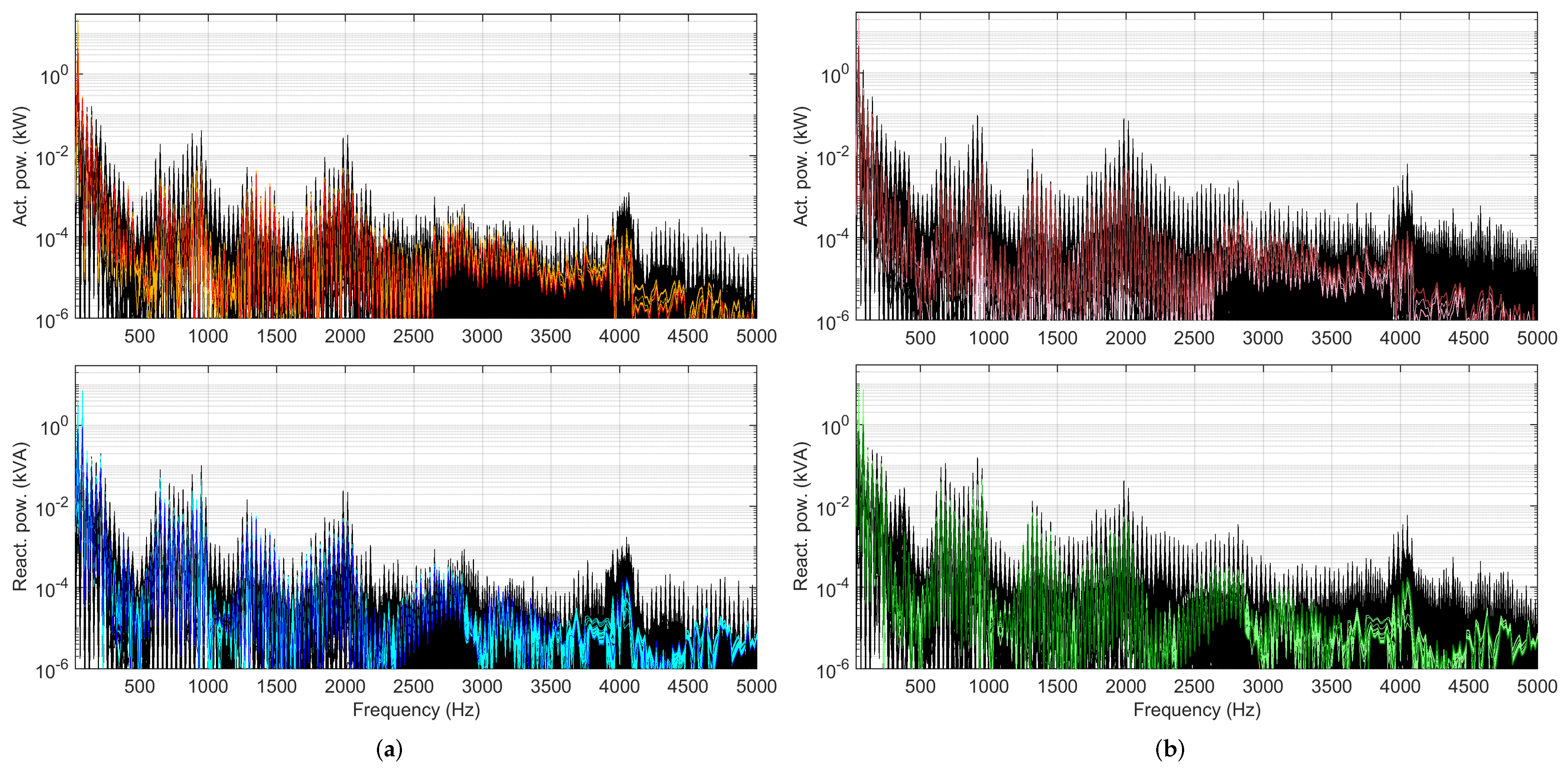
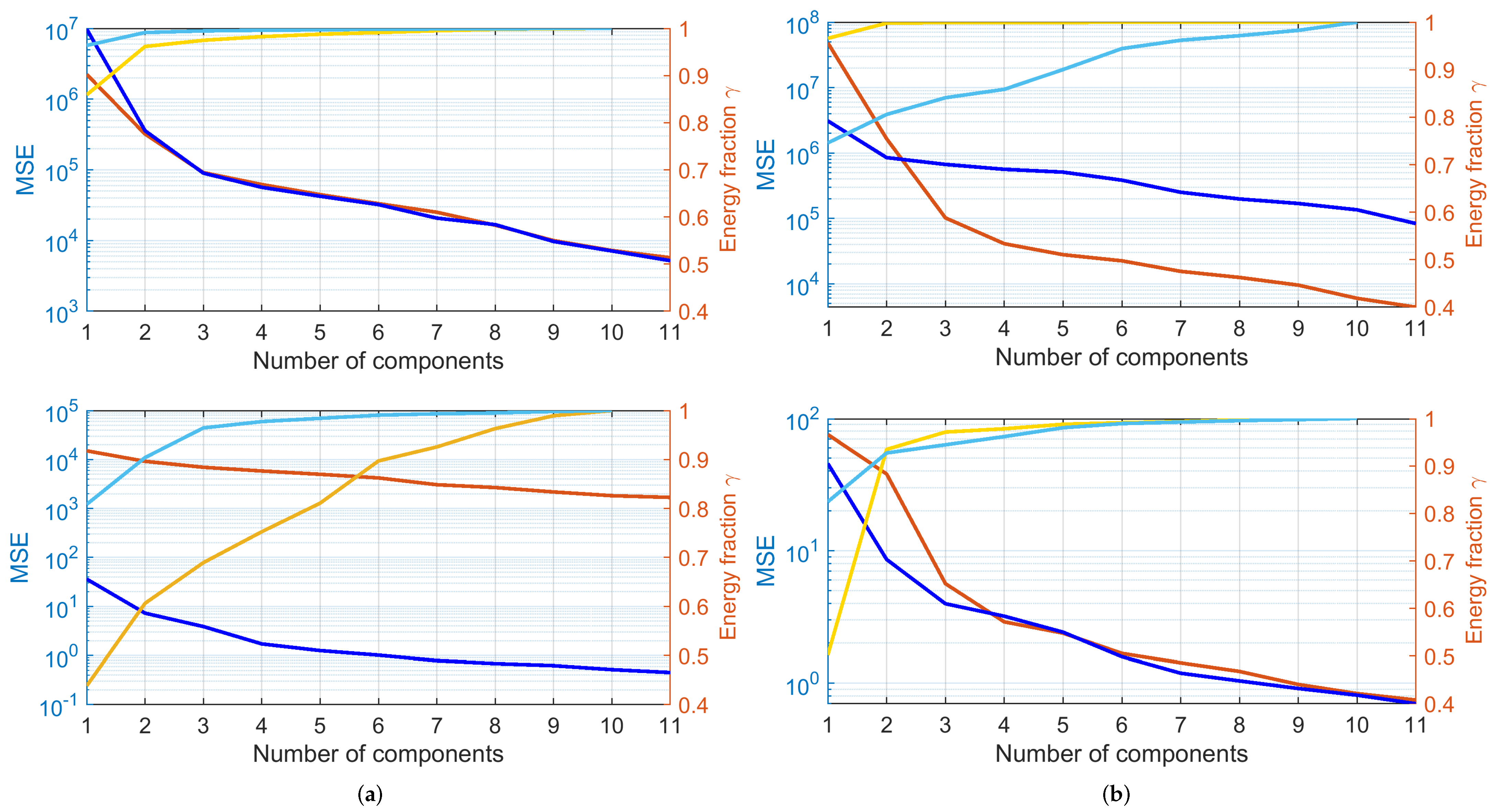
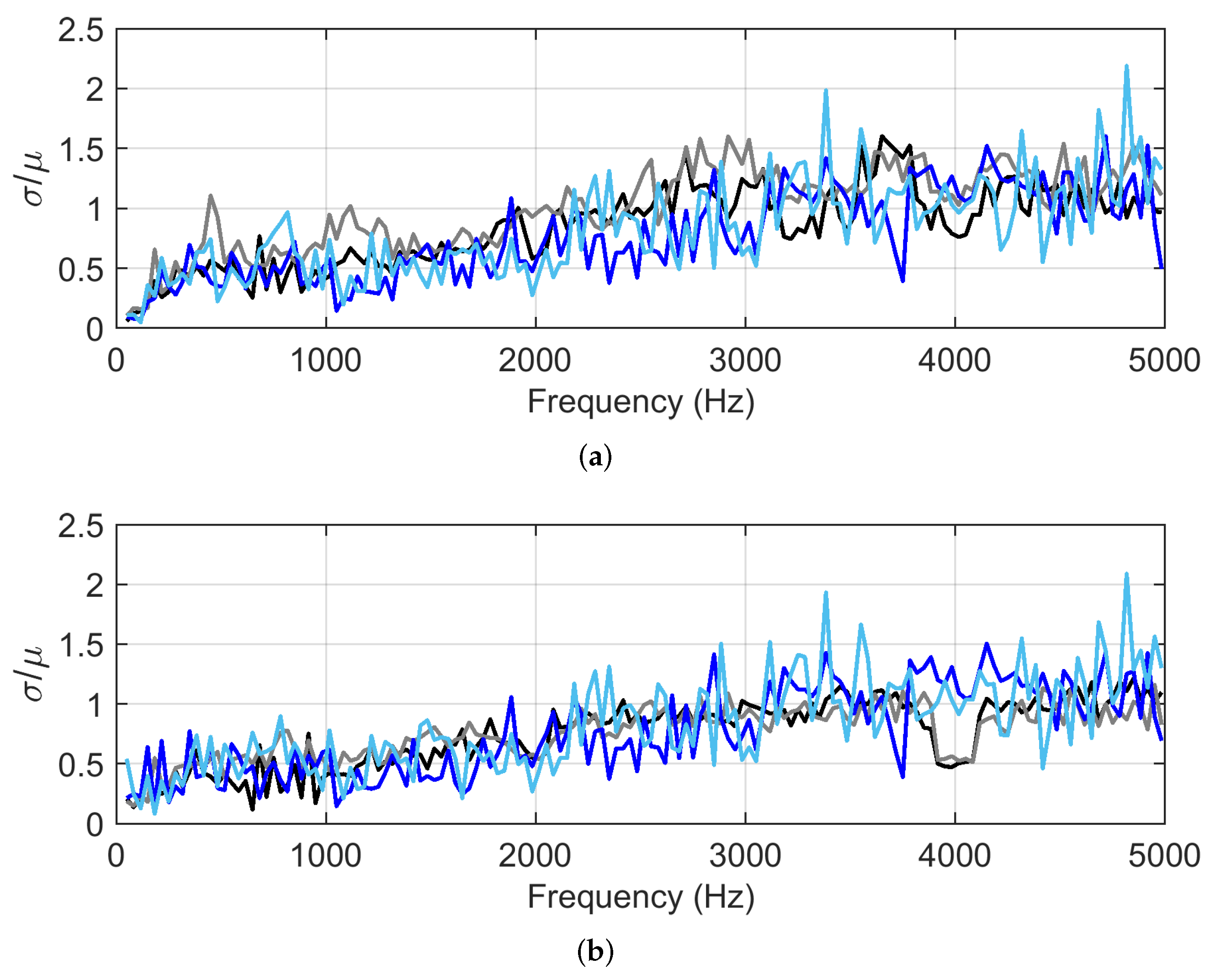
4.2. PCA Analysis and Spectra Regularity

$P_h$ and $Q_h$ spectra during a tractioning and braking interval have been analyzed for stationarity in terms of the number of independent components and their spatial distributions by means of PCA. For Swiss recordings, it is possible to conclude that:

• $P_h$ was described by only one main component, accounting for 99.86% of energy in tractioning and 99.90% in braking; adding the second one indicates 100% within four decimal digits;
• For $Q_h$, the same accuracy is reached with three components (99.88% of energy), but energy increase by adding successive components was much slower; the same performance of $P_h$ within four digits was reached at the 28th and 20th components for tractioning and braking conditions, respectively.

Three components were then retained for the graphical representations of the space distributions of $P_h$ and $Q_h$, shown in Figure 9.

With the principal components, identified on the ground of contribution to the total energy (e.g., individual variance), a simplified spectral representation can be retrieved, as shown in Figure 10.

Figure 10 shows (with the black background) the spread of the measured spectra, whereas the colored spectra are the PCA approximations, with the darker curve representing the average. It is evident that PCA “takes care” of components up to about $3.5$ kHz in traction conditions and 3 kHz in braking conditions. Reconstructed values are remarkably below the profiles of the measured spectra above the said frequency values, and even below them, there are voids here and there (namely, intervals where the provided PCA values are smaller than the measured ones). The reason may be due to a less coherent behavior of some components “filtered” by PCA, especially going toward the higher part of the spectrum; this is investigated further in the next section.

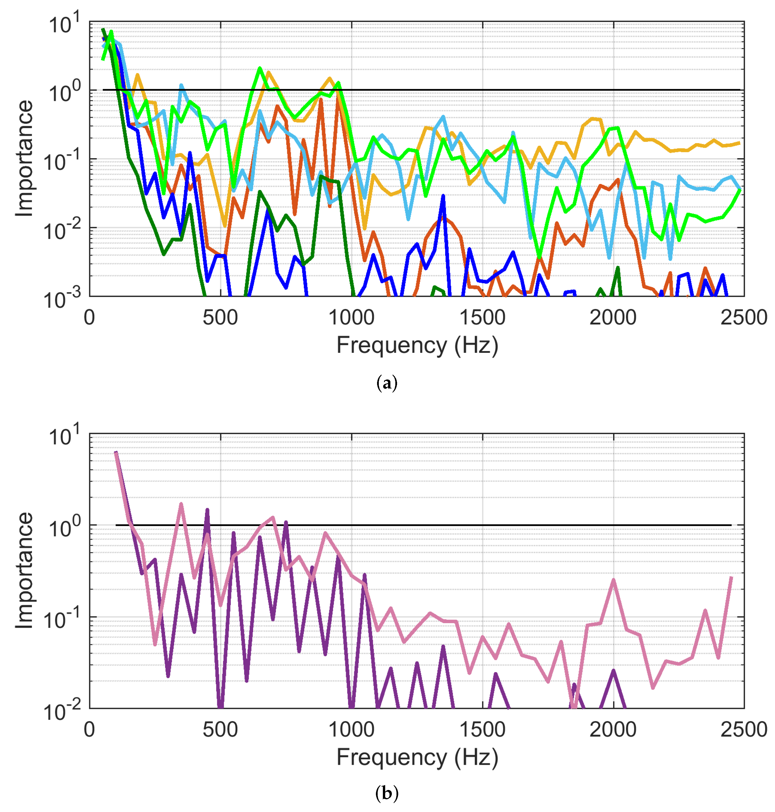
4.3. Selection of Spectral Components as Features

Rather than identifying complete spectrum traces as PCs extracted by PCA, the attention is now focused on spectrum subsets (e.g., a component or a group of components) to use as features for a clustering analysis. The objective is to identify those components with low intra-cluster variance and large inter-cluster variance.

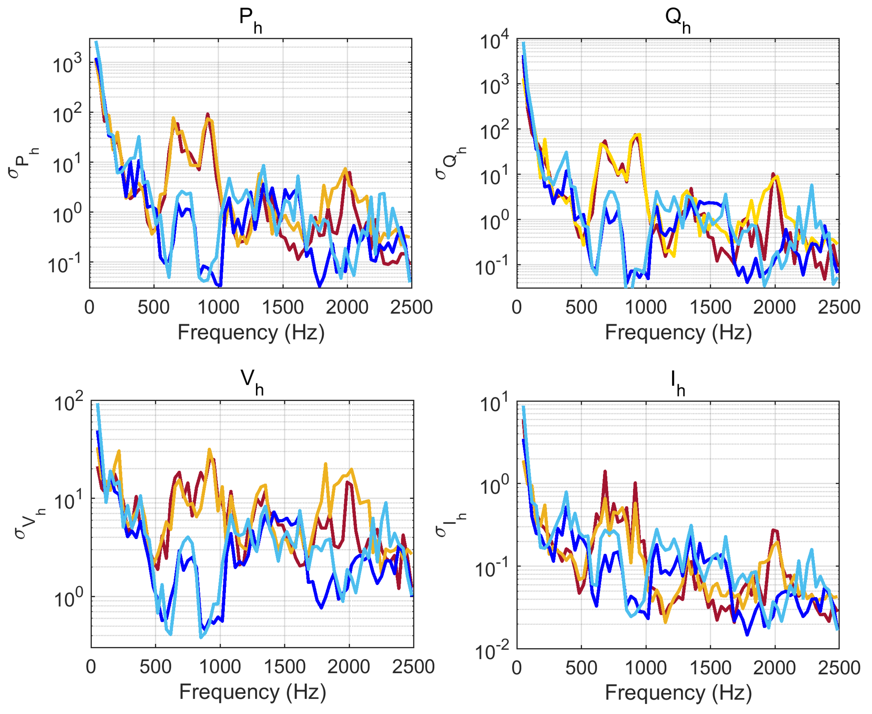
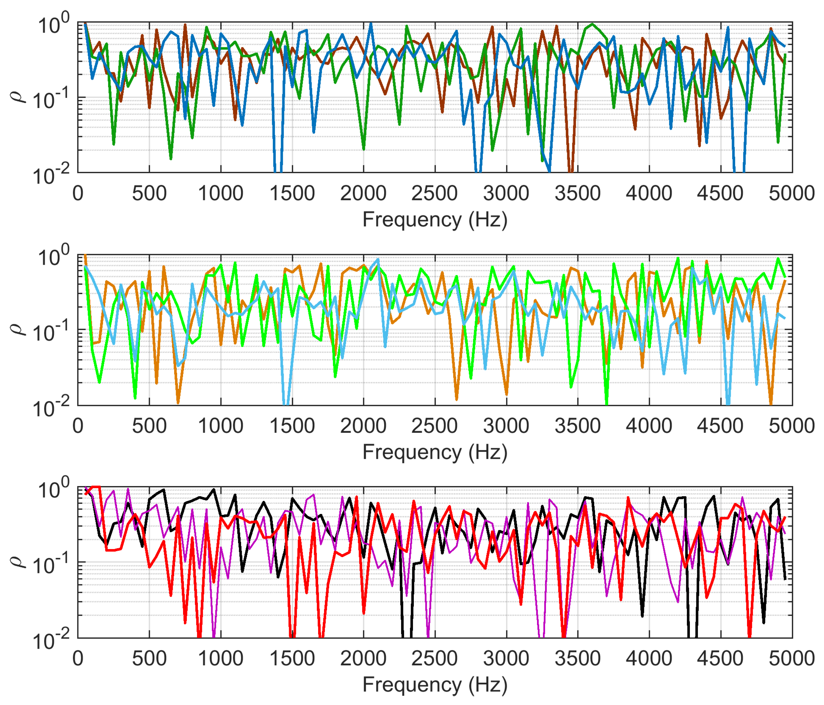
4.3.1. Dispersion and Correlation

This may be achieved by simply evaluating a sample variance for recordings labeled with the same or different operating conditions and rolling stock types. The sample variance is taken along index n for selected spectrum components, i.e., odd harmonics (even harmonics are known not to be characteristic harmonics in AC railways). To be selected as features, harmonics must have small intra- and large inter-variances for components belonging to the same and different operating conditions, respectively.

For the comparison between the different systems, despite the different values of the fundamental frequencies, spectra for $16.7$ Hz systems have been post-processed, obtaining one component out of three, and assigning it to the 50 Hz spaced grid. The options were an incoherent rms summation of the absolute value of the three components or the maximum value among the three, which preserve phase information (the latter was chosen).

Sample dispersions of spectra at each frequency bin were calculated, resulting in the coefficient of dispersion, $\sigma /\mu$, shown in Figure 11.

It is important to note that normalized dispersion increases significantly with frequency, implying that, if not suitably linked to variable operating conditions, such variability indicates simply excessive noise. As commented below, sources above about $2.5$ kHz are difficult to identify, for which reason the frequency interval of interest is limited to $2.5$ kHz, so as to achieve better frequency resolution and smaller matrices, where collected N observations have more relevant weights compared to the reduced M variables.

To appreciate the variability of spectra with respect to portions of the frequency interval, the sample dispersions were calculated separately for traction (dark colors) and braking (light colors) conditions, as shown in Figure 12.

This figure clarifies the influence of operating conditions on portions of the spectrum for each type of rolling stock. It was not constancy that we looked for, as the operating conditions were selected purposely to cover widely variable tractions and braking points; from a frequency domain perspective, it is interesting to observe which frequency intervals are influenced by varying operating points within traction or braking mode.

The curves confirm the significance of the 600 Hz to 900 Hz interval for the Swiss rolling stock, with a rebound of around 2 kHz, which is known to be secondary emissions caused by trains in the same supply section [53]. This underlines the importance of engineering judgment, avoiding blind assignment based on pure mathematical models, especially in realistic situations of mixed traffic (the Swiss rolling stock is in a normal commercial service on a very busy line). This is particularly evident as distortion in the $V_h$ spectrum, as these trains significantly pollute the line voltage, causing the discussed secondary emissions.

For the German rolling stock, the most significant emissions are located at 350 Hz to 450 Hz, with another significant burst at 700 Hz. It is interesting to observe the similarity of dispersion at about 350 Hz for both the Swiss and German rolling stocks. This is typical with older types of equipment, which likely run on the same line as the newer Swiss loco and pollute the line voltage, and (significantly) not the other quantities; conversely, this peak of dispersion is present in all four quantities for the older German train used for the tests, which has this frequency component among its characteristic emissions.

Another method of evaluation is estimating the correlation $\rho$ between the sets of measurements referred to as different operating conditions (traction and braking) and for different rolling stocks, as shown in Figure 13.

Correlation is calculated via the covariance matrix $\mathbf{G}$ for the considered sets of spectra belonging to the two compared, oc or rs, indicated as $\mathbf{U}$ and $\mathbf{V}$, made of M column vectors $u_m$ and $v_m$. Since for each frequency bin (along index m) the observation values form an $N\times 1$ vector that is not in principle related to other similar vectors for a different m value, the calculation of the correlation is carried out by orderly calculating the covariance matrix ${\mathbf{G}}_{\mathbf{m}}$ for each pair of vectors $u_m$ and $v_m$. ${\mathbf{G}}_{\mathbf{m}}$ is a $2\times 2$ matrix, from which the correlation coefficient ${\rho }_m$ may be determined.

$${\mathbf{G}}_{\mathbf{m}}=\mathrm{cov}({\mathbf{u}}_{\mathbf{m}},{\mathbf{v}}_{\mathbf{m}})=\left(\begin{array}{cc}{G}_{11}& G_{12}\\ G_{21}& G_{22}\end{array}\right)m=1,2,\dots M$$

(15)

$${\rho }_m=\frac{G_{12}}{\sqrt{G_{11}{G}_{22}}}m=1,2,\dots M$$

(16)

$$\rho (\mathbf{u},\mathbf{v})=[{\rho }_1,{\rho }_2,\dots {\rho }_m,\dots {\rho }_{M-1},{\rho }_M]$$

(17)

For simplicity, the correlation will be indicated only as $\rho$.

The purpose of Figure 13 is to show the correlation amounts between different sets of spectra belonging to one of the three types of rolling stocks (CH, D, or F, with obvious meaning) and two operating conditions (traction and braking).

The two 16.7 Hz systems should share some characteristics and show more similarities, but surprisingly the correlation values are large as for the cross-correlation with the French system.

Another point is that the same rolling stock in the two operating conditions (bottom subplot of Figure 13) should be more coherent than compared to the other subplots with cross-correlation terms. The reason is simply that, in many models, the converter used for traction and braking is the same, so characteristic harmonic groups should pop up. Moreover, this occurs for Switzerland (CH), featuring a large correlation between 500 and 900 Hz, where the 4QC operates, as well as for the German rolling stock (D) in the low-order harmonics range. However, it must be observed that correlation is calculated as a global index between all the recorded spectra of the traction subset and those of the braking subset, both undergoing a range of different operating points (namely different absorbed or released power, and different current intensities), which significantly shuffle scenarios. By removing the spectra with the lowest current intensity of nearly 20 A, the correlation improved slightly, as the number of PCA components was reduced by about 25%.

4.3.2. PLSR Analysis

The objective is to identify components that are the most relevant for the classification purpose, so attention is placed on a method that combines the projection of spectra on a compact space and ranks the most significant components.

Analogously to PCA, PLSR indicates the number of principal components along which data are represented and their performances in terms of incremental variance or energy fraction $\gamma$, as shown in Figure 14. Such “components” are spectral bins for PLSR and not entire projected spectrum vectors (as for PCA).

Only two components are sufficient in most cases to achieve a better-than-90% energy fraction $\gamma$. The most representative quantities are confirmed to be power terms $P_h$, $Q_h$, and current $I_h$.

As anticipated, PLSR indicates the most relevant components by means of the variable importance in projection (VIP), determined as the components that maximize the covariance between $\mathbf{X}$ and $\mathbf{y}$. Since the average of squared VIP scores equals 1, a commonly used criterion is to select components that have individual VIP scores larger than 1. This is shown in Figure 15 for the two 16.7 Hz systems (standalone, comparing the traction and braking conditions, and confronted, merging the traction and braking conditions for each).

By inspecting Figure 15a, the Swiss rolling stock is represented well by components between about 700 Hz and 950 Hz (where the Re460 converter emissions are located [14]), besides low-order harmonics that characterize all examined systems. When inspecting the combined curves (green), both these components and those around 350 Hz are judged relevant, the latter provided by the German train, as confirmed by the large value of its $I_h$ curve (light blue).

Figure 15b reports the result of the confrontation of the three systems, summarizing that components up to about 900 Hz are relevant. The relevance of the 2 kHz components, commented before as extraneous, but persistent, due to concomitant Swiss trains, has been correctly reduced. It should be noted that this comparison between heterogeneous spectra was made possible by transforming the spectra with 16.7 Hz harmonics of the CH and D systems into equivalent 50 Hz spectra by applying a max( ) operator to consecutive groups of three adjacent 16.7 Hz bins; this slightly reduces the resolution and representativeness.

It is worth noting that this last comparison shows the relevance of the $I_h$ spectrum (light violet curve), which has VIP values larger than the darker curve for $P_h$. This is important in the perspective of carrying out NILM at TPS, where the current is the quantity that can be more easily measured.

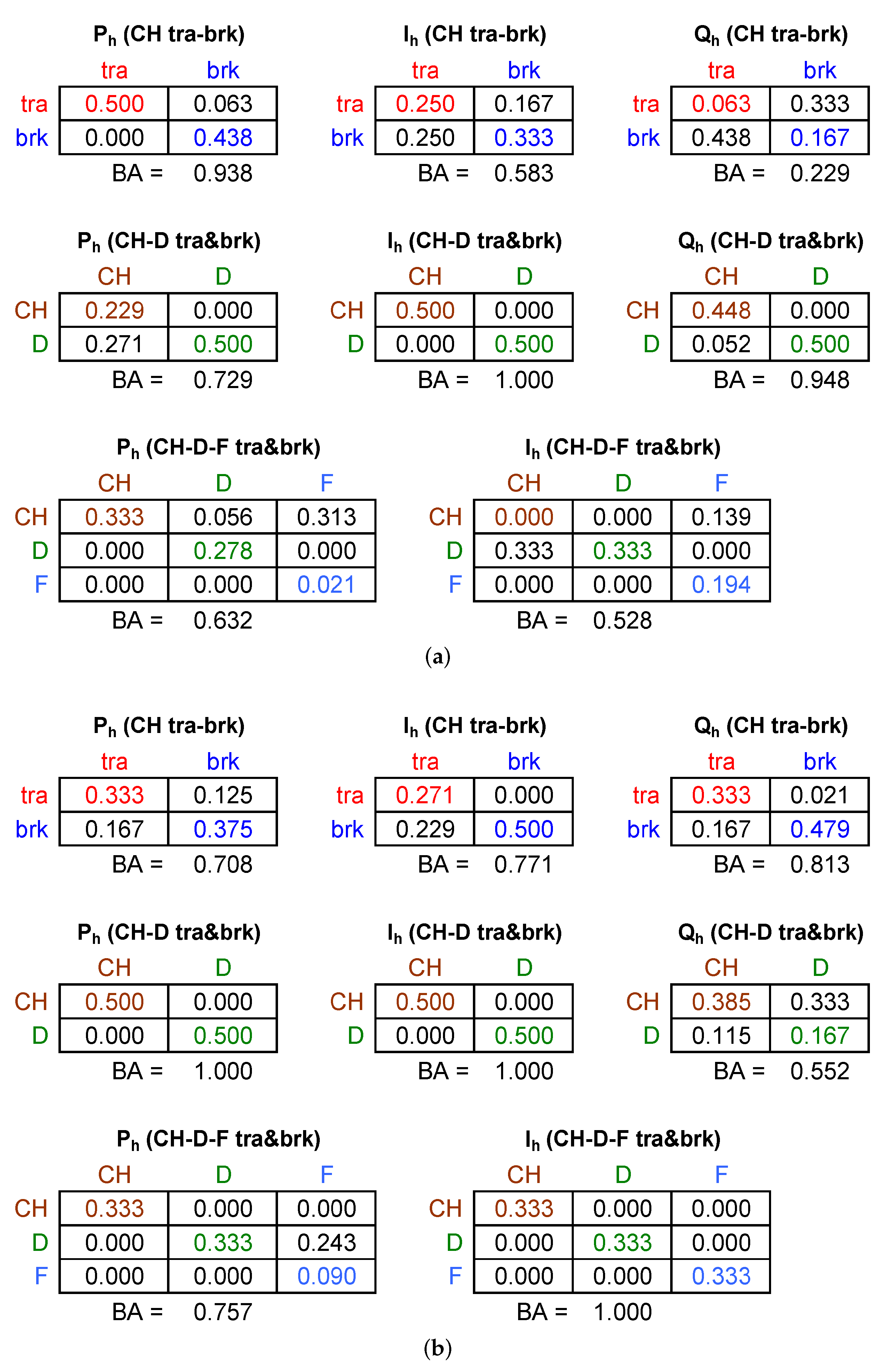
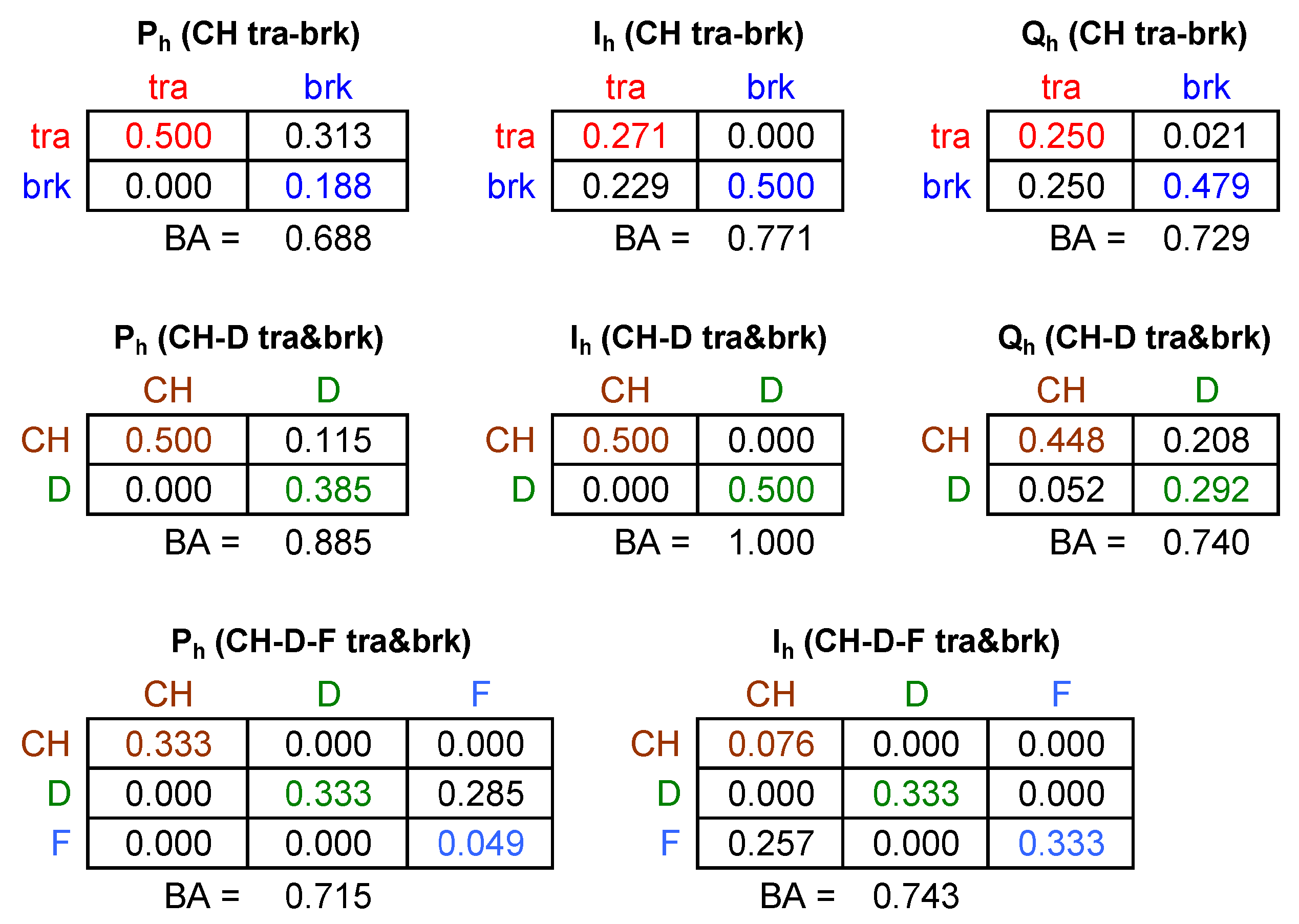
4.4. Classification Performance

The capabilities of the most promising indices reviewed so far were tested for classification purposes, using the same set of data on which the previous figures are based. Performance was measured by providing confusion matrices and balanced accuracy, as shown in Figure 16.

The main points are summarized as:

• Anticipated and demonstrated by other means, active power $P_h$ and current $I_h$ are the most effective indices; reactive power $Q_h$ also has good performance.
• The size of the problem is not an indicator of its complexity, as when systems are different, so their spectral signatures are; for the problem of separation of traction and braking for the same train, we saw the worst performance (the quantities are provided as absolute values, so removing the most relevant, but trivial, piece of information, i.e., the direction of flow).
• The current has a good understandable performance and is the best candidate to carry out NILM at the TPS.
• PLSR has a better performance than PCA, likely due to the dimensionality reduction.

For confirmation, clustering was also carried out with the GMM algorithm; in principle, it is more flexible than the k-means basic algorithm. Results are shown in Figure 17; surprisingly, the GMM algorithm performed worse, although not dramatically. There was a marginal improvement only for $Q_h$ for the CH-D clustering case.

5. Conclusions

This work focused on NILM applied to electrified transportation systems, focusing on AC railways, and considered a range of time domain and frequency domain indices:

• Voltage–current time domain trajectories provided poor performances because in the AC railway context, rolling stock has a strictly regulated displacement factor dictated by standards, so it does not represent a feature bearing relevant information for household NILM.
• Converter emissions are located at low-order harmonics and for more modern rolling stocks at the switching frequency of four-quadrant converters (4QCs), providing a feature-rich pattern of emissions up to about some kHz. For the analyzed case, the relevant frequency range extended up to 1 kHz, but there was evidence of an extraneous emission (explained by the presence of other trains in the same supply section) at 2 kHz, found relevant in one case at 4 kHz.
• Power and current harmonic spectra ($P_h$, $Q_h$, and $I_h$) were analyzed for significance with identification and classification purposes. The used methods spanned simple harmonic component tracking by means of sample dispersion and correlation, as well as principal component analysis (PCA) and partial least squares regression (PLSR) for extraction of more compact/better representations, aimed at clustering techniques.

After the identification of possible indices and features, and their preliminary verifications concerning their relationships with operating conditions, component separability, and variability, such features were verified by feeding them to clustering algorithms, assessing performance on a significant set of measured spectra. A total of 24 spectra for each operating condition (synthesized to traction and braking) and for each rolling stock (one for Switzerland, Germany, and France) were selected, 144 in total, to calculate statistics and clustering performances. Spectra were calculated based on the recordings available in the public dataset [52].

Assessed performances (via the confusion matrix) confirmed the better behavior of the PLSR algorithm in contrast to PCA, especially due to reduced dimensionality, which favors the clustering task. Then, even a basic clustering algorithm (such as k-means) has an almost optimal performance. Improved clustering algorithms (at least from a theoretical standpoint) were found to perform slightly worse, as demonstrated by using GMM in the same case.

Future developments involve confirming the findings using a larger set of data from other types of rolling stock and proceeding with data applications measured at TPS rather than at each rolling stock item. In addition, more powerful methods of spectra characterization may be explored, such as using higher-order cumulants, as well as pattern recognition techniques applied to 2D image-like representations, involving two quantities at the same time.

References

1. Zoha, A.; Gluhak, A.; Imran, M.; Rajasegarar, S. Non-Intrusive Load Monitoring Approaches for Disaggregated Energy Sensing: A Survey. Sensors 2012, 12, 16838–16866. [Google Scholar] [CrossRef] [Green Version]
2. Hassan, T.; Javed, F.; Arshad, N. An Empirical Investigation of V-I Trajectory Based Load Signatures for Non-Intrusive Load Monitoring. IEEE Trans. Smart Grid 2014, 5, 870–878. [Google Scholar] [CrossRef] [Green Version]
3. Herrero, J.R.; Murciego, Á.L.; Barriuso, A.L.; de la Iglesia, D.H.; González, G.V.; Rodríguez, J.M.C.; Carreira, R. Non Intrusive Load Monitoring (NILM): A State of the Art. In Advances in Intelligent Systems and Computing; Springer: Berlin/Heidelberg, Germany, 2017; pp. 125–138. [Google Scholar] [CrossRef]
4. Alqahtani, A.; Ali, M.; Xie, X.; Jones, M.W. Deep Time-Series Clustering: A Review. Electronics 2021, 10, 3001. [Google Scholar] [CrossRef]
5. Hosseini, S.S.; Agbossou, K.; Kelouwani, S.; Cardenas, A. Non-intrusive load monitoring through home energy management systems: A comprehensive review. Renew. Sustain. Energy Rev. 2017, 79, 1266–1274. [Google Scholar] [CrossRef]
6. Klemenjak, C.; Kovatsch, C.; Herold, M.; Elmenreich, W. A synthetic energy dataset for non-intrusive load monitoring in households. Sci. Data 2020, 7. [Google Scholar] [CrossRef] [Green Version]
7. Raygani, S.; Tahavorgar, A.; Fazel, S.; Moaveni, B. Load flow analysis and future development study for an AC electric railway. IET Electr. Syst. Transp. 2012, 2, 139. [Google Scholar] [CrossRef]
8. Mariscotti, A. Results on the power quality of French and Italian 2 × 25 kV 50 Hz railways. In Proceedings of the 2012 IEEE International Instrumentation and Measurement Technology Conference Proceedings, Graz, Austria, 13–16 May 2012; pp. 400–1405. [Google Scholar] [CrossRef]
9. Bongiorno, J.; Mariscotti, A. Recent results on the power quality of Italian 2 × 25 kV 50 Hz railways. In Proceedings of the 20th IMEKO TC4 Symposium on Measurements of Electrical Quantities, Benevento, Italy, 15–17 September 2014. [Google Scholar] [CrossRef]
10. Gazafrudi, S.M.M.; Langerudy, A.T.; Fuchs, E.F.; Al-Haddad, K. Power Quality Issues in Railway Electrification: A Comprehensive Perspective. IEEE Trans. Ind. Electron. 2015, 62, 3081–3090. [Google Scholar] [CrossRef]
11. Kaleybar, H.J.; Brenna, M.; Foiadelli, F.; Fazel, S.S.; Zaninelli, D. Power Quality Phenomena in Electric Railway Power Supply Systems: An Exhaustive Framework and Classification. Energies 2020, 13, 6662. [Google Scholar] [CrossRef]
12. Hanafy, A.M.; Hebala, O.M.; Hamad, M.S. Power Quality Issues in Traction Power Systems. In Proceedings of the 2021 22nd International Middle East Power Systems Conference (MEPCON), Luxor City, Egypt, 14–16 December 2021. [Google Scholar] [CrossRef]
13. Seferi, Y.; Blair, S.M.; Mester, C.; Stewart, B.G. Power Quality Measurement and Active Harmonic Power in 25 kV 50 Hz AC Railway Systems. Energies 2020, 13, 5698. [Google Scholar] [CrossRef]
14. Mariscotti, A. Experimental characterisation of active and non-active harmonic power flow of AC rolling stock and interaction with the supply network. IET Electr. Syst. Transp. 2021, 11, 109–120. [Google Scholar] [CrossRef]
15. Lam, H.; Fung, G.; Lee, W. A Novel Method to Construct Taxonomy Electrical Appliances Based on Load Signaturesof. IEEE Trans. Consum. Electron. 2007, 53, 653–660. [Google Scholar] [CrossRef] [Green Version]
16. Kosarev, A.P.; Volkov, A.G.; Zinoviev, G.S. Analysis of new multizone rectifier for electric locomotives of V185 type. In Proceedings of the 2010 11th International Conference and Seminar on Micro/Nanotechnologies and Electron Devices, Novosibirsk, Russia, 30 June–4 July 2010. [Google Scholar] [CrossRef]
17. Chang, G.; Lin, H.W.; Chen, S.K. Modeling Characteristics of Harmonic Currents Generated by High-Speed Railway Traction Drive Converters. IEEE Trans. Power Deliv. 2004, 19, 766–773. [Google Scholar] [CrossRef]
18. Van der Weem, J.; Bolln, H. Measurement and analysis of line interference currents generated by an IGBT four quadrant converter. In Proceedings of the 2005 European Conference on Power Electronics and Applications, Dresden, Germany, 11–14 September 2005. [Google Scholar] [CrossRef]
19. He, Z.; Zheng, Z.; Hu, H. Power quality in high-speed railway systems. Int. J. Rail Transp. 2016, 4, 71–97. [Google Scholar] [CrossRef] [Green Version]
20. Florio, A.; Mariscotti, A.; Mazzucchelli, M. Voltage Sag Detection Based on Rectified Voltage Processing. IEEE Trans. Power Deliv. 2004, 19, 1962–1967. [Google Scholar] [CrossRef]
21. Kamble, S.; Thorat, C. Voltage Sag Characterization in a Distribution Systems: A Case Study. J. Power Energy Eng. 2014, 2, 546–553. [Google Scholar] [CrossRef]
22. Santis, M.D.; Noce, C.; Varilone, P.; Verde, P. Analysis of the origin of measured voltage sags in interconnected networks. Electr. Power Syst. Res. 2018, 154, 391–400. [Google Scholar] [CrossRef]
23. Liang, J.; Ng, S.K.K.; Kendall, G.; Cheng, J.W.M. Load Signature Study — Part I: Basic Concept, Structure, and Methodology. IEEE Trans. Power Deliv. 2010, 25, 551–560. [Google Scholar] [CrossRef]
24. Cardenas, A.; Agbossou, K.; Guzman, C. Development of real-time admittance analysis system for residential load monitoring. In Proceedings of the 2016 IEEE 25th International Symposium on Industrial Electronics (ISIE), Santa Clara, CA, USA, 8–10 June 2016. [Google Scholar] [CrossRef]
25. Ruano, A.; Hernandez, A.; Ureña, J.; Ruano, M.; Garcia, J. NILM Techniques for Intelligent Home Energy Management and Ambient Assisted Living: A Review. Energies 2019, 12, 2203. [Google Scholar] [CrossRef] [Green Version]
26. Ester, M.; Kriegel, H.P.; Sander, J.; Xu, X. A density-based algorithm for discovering clusters in large spatial databases with noise. In Proceedings of the Second International Conference on Knowledge Discovery and Data Mining, Portland, OR, USA, 2–4 August 1996; pp. 226–231. [Google Scholar]
27. Schubert, E.; Sander, J.; Ester, M.; Kriegel, H.P.; Xu, X. DBSCAN Revisited, Revisited. ACM Trans. Database Syst. 2017, 42, 1–21. [Google Scholar] [CrossRef]
28. Zhang, J.; Shang, J.; Zhang, Z. Optimization and Control on High Frequency Resonance of Train-Network Coupling Systems. Math. Probl. Eng. 2019, 2019, 1–10. [Google Scholar] [CrossRef] [Green Version]
29. Mariscotti, A.; Ruscelli, M.; Vanti, M. Modeling of audiofrequency track circuits for validation, tuning, and conducted interference prediction. IEEE Trans. Intell. Transp. Syst. 2009, 11, 52–60. [Google Scholar] [CrossRef]
30. Dolara, A.; Gualdoni, M.; Leva, S. EMC disturbances on track circuits in the 2 × 25 kV high speed AC railways systems. In Proceedings of the 2011 IEEE Trondheim PowerTech, Trondheim, Norway, 19–23 June 2011. [Google Scholar] [CrossRef]
31. Mariscotti, A. Induced Voltage Calculation in Electric Traction Systems: Simplified Methods, Screening Factors, and Accuracy. IEEE Trans. Intell. Transp. Syst. 2011, 12, 201–210. [Google Scholar] [CrossRef]
32. Milesevic, B.; Haddad, N. Estimation of current through human body in case of contact with pipeline in the vicinity of a 50 Hz electrified railway. In Proceedings of the 2013 International Symposium on Electromagnetic Compatibility, Brugge, Belgium, 2–6 September 2013. [Google Scholar]
33. Gao, S.; Li, X.; Ma, X.; Hu, H.; He, Z.; Yang, J. Measurement-Based Compartmental Modeling of Harmonic Sources in Traction Power-Supply System. IEEE Trans. Power Deliv. 2017, 32, 900–909. [Google Scholar] [CrossRef]
34. Yang, R.; Zhou, F.; Zhong, K. A Harmonic Impedance Identification Method of Traction Network Based on Data Evolution Mechanism. Energies 2020, 13, 1904. [Google Scholar] [CrossRef] [Green Version]
35. Mariscotti, A.; Sandrolini, L. Detection of harmonic overvoltage and resonance in AC railways using measured pantograph electrical quantities. Energies 2021, 14, 5645. [Google Scholar] [CrossRef]
36. Wang, J.; Yang, Z.; Lin, F.; Cao, J. Harmonic Loss Analysis of the Traction Transformer of High-Speed Trains Considering Pantograph-OCS Electrical Contact Properties. Energies 2013, 6, 5826–5846. [Google Scholar] [CrossRef] [Green Version]
37. EN 50463-2; Railway Applications—Energy Measurement on Board Trains. Technical report; CENELEC: Brussels, Belgium, 2017.
38. Mariscotti, A. Impact of Harmonic Power Terms on the Energy Measurement in AC Railways. IEEE Trans. Instrum. Meas. 2020, 69, 6731–6738. [Google Scholar] [CrossRef]
39. Giordano, D.; Clarkson, P.; Gamacho, F.; van den Brom, H.; Donadio, L.; Fernandez-Cardador, A.; Spalvieri, C.; Gallo, D.; Istrate, D.; Laporte, A.D.S.; et al. Accurate Measurements of Energy, Efficiency and Power Quality in the Electric Railway System. In Proceedings of the 2018 Conference on Precision Electromagnetic Measurements (CPEM 2018), Paris, France, 8–13 July 2018. [Google Scholar] [CrossRef]
40. Hasegawa, D.; Nicholson, G.L.; Roberts, C.; Schmid, F. Standardised approach to energy consumption calculations for high-speed rail. IET Electr. Syst. Transp. 2016, 6, 179–189. [Google Scholar] [CrossRef]
41. Hemmer, B.; Mariscotti, A.; Wuergler, D. Recommendations for the calculation of the total disturbing return current from electric traction vehicles. IEEE Trans. Power Deliv. 2004, 19, 1190–1197. [Google Scholar] [CrossRef]
42. IEEE Std. 1459; IEEE Standard Definitions for the Measurement of Electric Power Quantities Under Sinusoidal, Nonsinusoidal, Balanced, or Unbalanced Conditions. IEEE: Piscataway, NJ, USA, 2010.
43. Mariscotti, A. Behavior of single-point harmonic producer indicators in electrified ac railways. Metrol. Meas. Syst. 2020, 27, 641–657. [Google Scholar] [CrossRef]
44. Tenti, P.; Mattavelli, P. A Time-Domain Approach to Power Term Definitions under Non-Sinusoidal Conditions. In Proceedings of the Sixth International Workshop on Power Definitions and Measurements under Non-Sinusoidal Conditions, Milano, Italy, 13–15 October 2003. [Google Scholar]
45. Mariscotti, A. Harmonic and Supraharmonic Emissions of Plug-In Electric Vehicle Chargers. Smart Cities 2022, 5, 496–521. [Google Scholar] [CrossRef]
46. EN 50388; Railway Applications—Power Supply and Rolling Stock—Technical Criteria for the Coordination between Power Supply (Substation) and Rolling Stock to Achieve Interoperability. Technical report; CENELEC: Brussels, Belgium, 2012.
47. Jolliffe, I.T.; Cadima, J. Principal component analysis: A review and recent developments. Philos. Trans. R. Soc. Math. Phys. Eng. Sci. 2016, 374, 20150202. [Google Scholar] [CrossRef] [PubMed]
48. Abdi, H. Encyclopedia of Social Sciences Research Methods; Chapter Partial Least Squares (PLS) Regression; Sage: Newbury Park, CA, USA, 2003. [Google Scholar]
49. De Jong, S. SIMPLS: An alternative approach to partial least squares regression. Chemom. Intell. Lab. Syst. 1993, 18, 251–263. [Google Scholar] [CrossRef]
50. Hughes, G. On the mean accuracy of statistical pattern recognizers. IEEE Trans. Inf. Theory 1968, 14, 55–63. [Google Scholar] [CrossRef] [Green Version]
51. Aha, D.W.; Kibler, D.; Albert, M.K. Instance-Based Learning Algorithms. Mach. Learn. 1991, 6, 37–66. [Google Scholar] [CrossRef] [Green Version]
52. Mariscotti, A. Data sets of measured pantograph voltage and current of European AC railways. Data Brief 2020, 30, 105477. [Google Scholar] [CrossRef] [PubMed]
53. Mariscotti, A. Direct measurement of power quality over railway networks with results of a 16.7-Hz network. IEEE Trans. Instrum. Meas. 2010, 60, 1604–1612. [Google Scholar] [CrossRef]
Figure 1. Example of the VI diagram and explanatory symbols for the locus features: blue circles for current extremes I max and I min , joined by the dashed extreme line; purple squares for voltage extremes V max and V min ; intersections with the vertical axis indicated by the brown crosses ( i 0 + and i 0 ); self intersections indicated by green circles; black curve for the mean curve.
Energies 15 04141 g001
Figure 2. Example of data arrangement for PCA analysis.
Energies 15 04141 g002
Figure 3. Graphical description of the confusion matrix C : a and b are the row and column indices, α and β are the positions of the specific cells (the first one in this example is for graphical reasons), summation expressions indicate how to revert to a binary confusion matrix representation.
Energies 15 04141 g003
Figure 4. Typical VI trajectories for Switzerland (from low to high current intensities, top to bottom): (a) tractioning, (b) braking.
Energies 15 04141 g004
Figure 5. Typical VI trajectories for Germany (from low to high current intensities, top to bottom): (a) tractioning, (b) braking.
Energies 15 04141 g005
Figure 6. Typical VI trajectories for France (from low to high current intensities, top to bottom): (a) tractioning, (b) braking.
Energies 15 04141 g006
Figure 7. Scatter plot of normalized A and I 0 . The traction conditions are indicated by dark green, blue, and red for CH, D, and F, respectively; similarly, braking conditions have corresponding lighter nuances.
Energies 15 04141 g007
Figure 8. Scatter plot of the normalized ξ and ψ . The traction conditions on the right-hand side are indicated by dark green, blue, and red for CH, D, and F, respectively; similarly, braking conditions on the left-hand side have corresponding lighter nuances.
Energies 15 04141 g008
Figure 9. Spatial distribution of the first three PCA components for P h and Q h : (a) tractioning, (b) braking.
Energies 15 04141 g009
Figure 10. Spectral approximation of the first three PCA components for P h and Q h : (a) tractioning, (b) braking; the darker colored trace is the mean of the PCA approximation (in lighter color).
Energies 15 04141 g010
Figure 11. Normalized dispersion σ / μ , calculated out of 24 + 24 observations for traction and braking conditions for: (a) P h and Q h (black and grey for CH, blue and light blue for D system, respectively); (b) V h and I h (black and grey for CH, blue and light blue for D system, respectively).
Energies 15 04141 g011
Figure 12. Dispersion σ , calculated out of 24 + 24 observations for traction (dark colors) and braking (light colors) conditions: CH brown, D blue.
Energies 15 04141 g012
Figure 13. Correlation between groups of spectra: cross-correlation in traction (top) and braking (middle) conditions (CH vs. D (brown), CH vs. F (blue), and D vs. F (green)); cross-correlation between traction and braking conditions for the same rolling stock (CH (black), D (violet), F (red)).
Energies 15 04141 g013
Figure 14. PLSR results for fitting quality (mean square error, MSE) and cumulative energy fraction γ : (a) traction and braking classes for Switzerland; (b) distinction of the three rolling stock for Switzerland, Germany, and France (traction and braking conditions altogether). P h (brown dark and light), and Q h (blue dark and light) above, V h (brown dark and light), and I h (blue dark and light) below.
Energies 15 04141 g014
Figure 15. PLSR VIP scores for (a) 16.7 Hz system representation (CH tra-brk brown dark and light, D tra-brk blue dark, and combined CH and D green dark and light light, (b) combined 16.7 Hz and 50 Hz system representation (Switzerland, Germany, and France); dark and light refer to P h and I h ).
Energies 15 04141 g015
Figure 16. Confusion matrices and balanced accuracy BA for (a) PCA and (b) PLSR, using the k-means algorithm: 24 observations used for each rs (CH, D, and F train) and oc (traction and braking) for a total of 144 spectra; comparisons were carried out for traction/braking conditions within the same system (selected CH), for different rs for more similar systems (CH and D), and the same for all three different systems (CH, D, and F).
Energies 15 04141 g016
Figure 17. Confusion matrices and balanced accuracy BA for PLSR using the GMM algorithm: 24 observations used for each rs (CH, D, and F train) and oc (traction and braking) for a total of 144 spectra; comparisons were carried out for traction/braking conditions within the same system (selected CH), for different rs for more similar systems (CH and D), and the same for all three different systems (CH, D, and F).
Energies 15 04141 g017