Synthesis of Driving Cycles Based on Low-Sampling-Rate Vehicle-Tracking Data and Markov Chain Methodology

Abstract

The authors of this paper propose a Markov-chain-based method for the synthesis of naturalistic, high-sampling-rate driving cycles based on the route segment statistics extracted from low-sampling-rate vehicle-tracking data. In the considered case of a city bus transport system, the route segments correspond to sections between two consecutive bus stations. The route segment statistics include segment lengths and maps of average velocity, station stop time, and station-stopping probability, all given along the day on an hourly basis. In the process of driving cycle synthesis, the transition probability matrix is built up based on the high-sampling-rate driving cycles purposely recorded in a separate reference city. The particular emphasis of the synthesis process is on satisfying the route segment velocity and acceleration boundary conditions, which may be equal to or greater than zero depending on whether a bus stops or passes a station. This enables concatenating the synthesized consecutive micro-cycles into the full-trip driving cycle. The synthesis method was validated through an extensive statistical analysis of generated driving cycles, including computational efficiency aspects.

1. Introduction

Increasing environmental awareness has been a key initiator of stricter regulations towards reductions in vehicle energy consumption and greenhouse gas emissions [1]. A vehicle’s energy consumption and related emissions strongly depend on the driving cycle [2,3,4], which is usually defined as the vehicle speed vs. time profile [5,6]. As such, it represents a characteristic driving pattern that reflects driver behavior (e.g., driving aggressiveness) and road conditions (road type, road slope, traffic conditions, etc.) [7,8]. From the early 1960s, specific, so-called certification driving cycles have served as input to standardized emissions and energy-consumption-related certification processes worldwide [4,5]. They can also be used to select optimal vehicle powertrain configurations and develop optimal vehicle control strategies [9,10], as well as to determine effective vehicle range, battery life expectancy, and optimal charging management strategies in the case of electric vehicles [11,12,13,14]. Therefore, the driving cycles should represent the actual driving behavior and road conditions as much as possible [15].

Although the certification processes have been proven to be successful in facilitating continuous reductions in vehicle energy consumption and greenhouse gas emissions, a significant gap has been observed between energy-consumption rates obtained for certification driving cycles and real driving conditions [16,17,18]. To reduce this gap, recent research efforts have been focused on developing statistically representative synthetic driving cycles derived from GPS-recorded vehicle-tracking data [19,20]. The main aim of driving cycle synthesis is to replace a wide set of recorded driving cycles with a single or several synthetic cycles that are statistically representative in terms of reflecting the average driving pattern of the initial (recorded) set.

The most common approach to the synthesis of driving cycles is based on the Markov chain stochastic method [21,22,23]. Its main advantages over micro-trip-based methods [24,25] are its (i) flexibility of generating a synthetic driving cycle with a desired travel time or total distance traveled [19,20] and (ii) inherent ability to solve the problem of missing GPS data through omitting the irregular transitions between Markov states when determining the driving-cycle model in the form of a transition probability matrix (TPM). By means of repetitive random sampling from a TPM, it is possible to generate an unlimited number of synthetic driving cycles [26]. Finally, applying certain validation criteria enables the extraction of the synthetic driving cycles that are most representative in the statistical sense [27,28].

For the aforementioned vehicle testing and simulation applications (see also [29,30]), the driving cycles should be synthesized based on input data of a high sampling rate (at least 1 Hz). However, widely deployed GPS tracking devices broadcast data at a significantly lower sampling rate, which is typically in the range from 0.025 to 0.2 Hz [31]. The issue can be overcome n the following distinct ways: (i) adjusting the tracking device hardware or software to allow for high-rate broadcasting [20,32,33] and (ii) developing a synthesis method that could generate high-sampling-rate (HSR) driving cycles from the low-sampling-rate (LSR) input database. The former imposes additional workload and/or cost and is subject to permission by the transport company. The latter is generally more convenient because it relies on readily available tracking data, but it also requires the development of a specific driving cycle generation method, which is the main subject of this paper.

The proposed method consists of three distinctive steps. Firstly, the LSR data are post-processed to obtain the route/trip segment statistics in terms of segment length and maps of average velocity, station stop time, and station-stopping probability given along the day on an hourly basis. In the particular case of the city bus transport system, the trip segments correspond to road sections between two consecutive bus stations at which the bus may or may not stop. Secondly, HSR tracking data recorded in a separate (reference, “donor”) city are split into the trip segment micro-cycles, which are used to build the TPM model. For numerical efficiency reasons, the TPM model is represented by a number of TPMs corresponding to different clusters of recorded micro-cycles in terms of mean velocity. Thirdly, the post-processed LSR data and the HSR TPM model are used to synthesize the HSR driving cycles. The synthesis is essentially conducted over the trip segments to match the LSR data segment statistics. By providing that the vehicle velocity and acceleration boundary conditions (i.e., initial and final conditions) are satisfied, the synthesized trip segment micro-cycles can be readily concatenated into the final, full trip driving cycle. While the Markov-chain-based driving cycle synthesis method itself is well-known [32,33,34], its use to generate trip-segment micro-cycles that satisfy the LSR data statistical features and provide the zero or non-zero boundary conditions has not been addressed in the available literature.

The main contributions of the paper include: (i) a general framework for synthesizing HSR driving cycles based on readily available LSR fleet tracking data and a reference HSR recorded driving cycle database; (ii) a micro-cycle synthesis method that satisfies the prescribed velocity and acceleration boundary conditions while accounting for the multi-TPM micro-cycle model.

The paper is organized as follows. Section 2 describes the considered city bus transport system, outlines the motivation and requirements for the synthesis of HSR driving cycles from LSR tracking data, and presents the LSR tracking data-based traffic model. Section 3 briefly describes the standard Markov chain method for the synthesis of naturalistic driving cycles. Section 4 elaborates the proposed trip segment-based HSR driving cycle synthesis method, which satisfies the predetermined LSR data’s statistical features and related boundary conditions. Section 5 deals with the validation of the proposed driving cycle synthesis method. Concluding remarks are given in Section 6.

2. Problem Description

2.1. On Importance of Microsimulations for Transport Electrification Planning Purposes

Transport system operators, e.g., those managing city bus or delivery fleets, experience pressure to reduce the number of vehicles and fuel/energy-consumption costs through proper fleet scheduling/routing [35]. The introduction of electrified transport systems led to the need for even more comprehensive planning because of the limited e-vehicle range and the need to optimally deploy a charging infrastructure [29].

Since the energy consumption of future electrified transport system cannot be known in advance, planning studies can be conducted based on virtual (computer) microsimulations that rely on physical vehicle models and available (historical) GPS vehicle-tracking data [29]. The main advantage of such a microsimulation approach is that it provides accurate energy-consumption estimates for a wide range of road and ambient conditions when using experimentally validated vehicle models. However, it requires driving cycles recorded at a high sampling rate (HSR; typically around 1 Hz) even though the fleet operators routinely make recordings at orders-of-magnitude lower sampling rates (LSRs). Therefore, there is a necessity to develop a method that could synthesize HSR driving cycles for a target (“acceptor”) transport system, whose statistical features correspond to the recorded LSR data of the same system, and replicate the features of HSR driving cycles purposely recorded in a separate reference (“donor”) transport system with similar characteristics. Such a method is proposed in this paper based on a Markov chain synthesis method and demonstrated with an example city bus transport system.

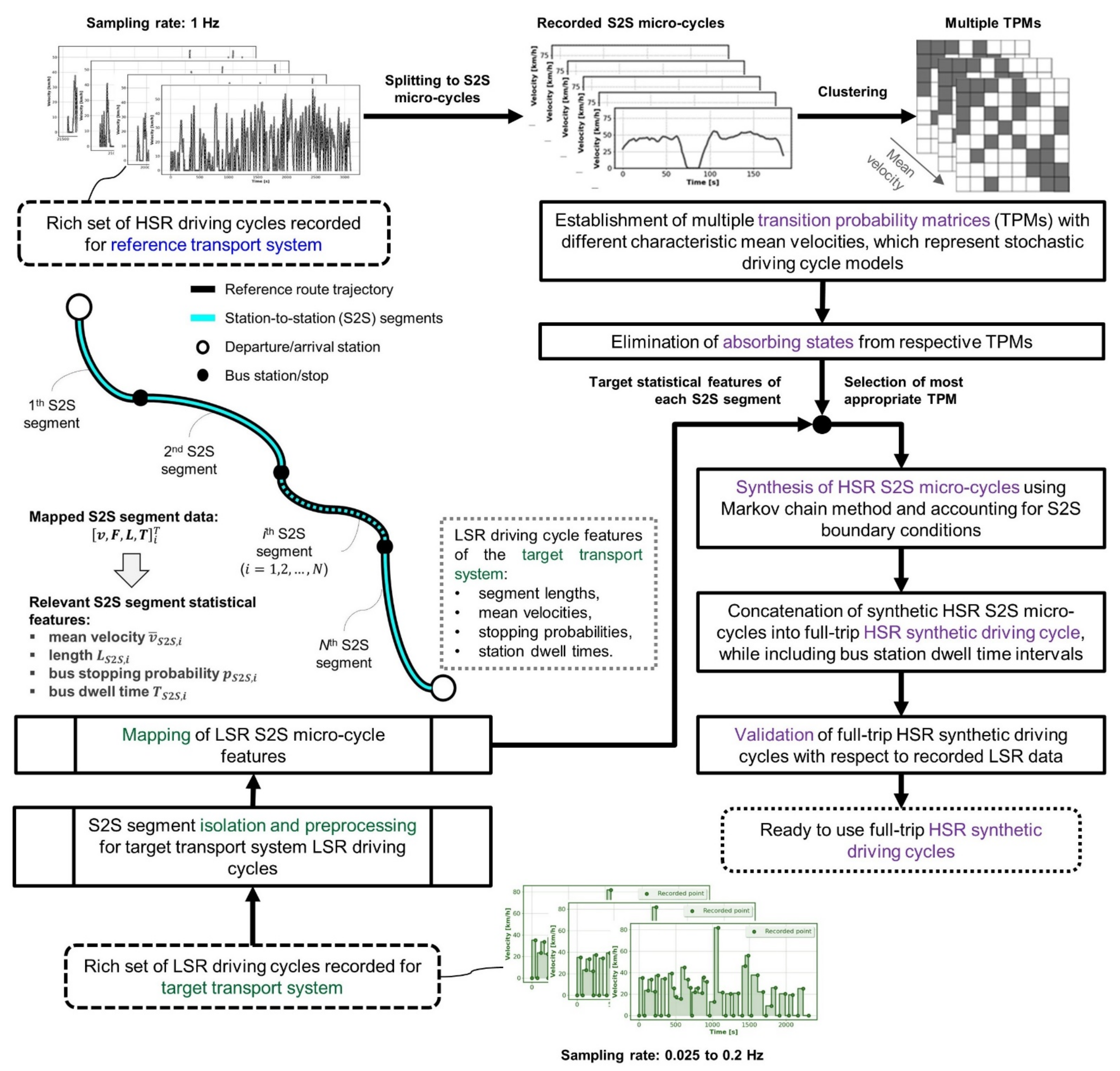
2.2. High-Sampling-Rate (HSR) Driving Cycle Synthesis Framework

Figure 1 illustrates the overall framework of the HSR driving cycle synthesis proposed in this paper. The initial step involved splitting a rich set of already available recorded HSR driving cycles of the reference city bus transport system (corresponding to the city of Dubrovnik; see [28,29,34]) into bus station-to-station (S2S) segments. This allowed for the isolation of a large set of HSR micro-cycles, where each micro-cycle was described by vehicle velocity vs. time profile corresponding to an S2S segment. The extracted HSR micro-cycles were then clustered according to their mean velocities and used for establishing multiple stochastic driving-cycle models represented by transition probability matrices (TPMs).

The next step comprised the mapping of the recorded LSR driving cycle data for the target city bus transport system (related to the city of Jerusalem in this paper) into relevant statistical features over the S2S segments. The statistical features included the ith S2S segment length $L_{S2S,i}$ and the corresponding spatial–temporal maps of mean velocity $\left({\overline{v}}_{S2S,i}\right)$, station dwell time $(T_{S2S,i})$, and station-stopping probability $(p_{S2S,i})$.

The final step comprised the generation of target city HSR S2S micro-cycles that matched the reference city TPM model and the LSR driving cycle features (Section 4). The generation process was based on the Markov chain synthesis method (Section 3). The generated micro-cycles also needed to satisfy the S2S velocity boundary conditions. The full-trip HSR synthetic driving cycles were then obtained by concatenating the synthetic S2S micro-cycles and inserting station idle pauses in accordance with the LSR driving cycle features. The representativeness of such generated HSR synthetic driving cycles was finally confirmed by their validation with respect to recorded LSR data (Section 5).

2.3. Requirements on Process of Generating HSR Driving Cycles

The following minimalistic LSR dataset was required to establish the target transport system traffic model and ultimately obtain the HSR synthetic driving cycles (see Figure 2 for details of the overall procedure):

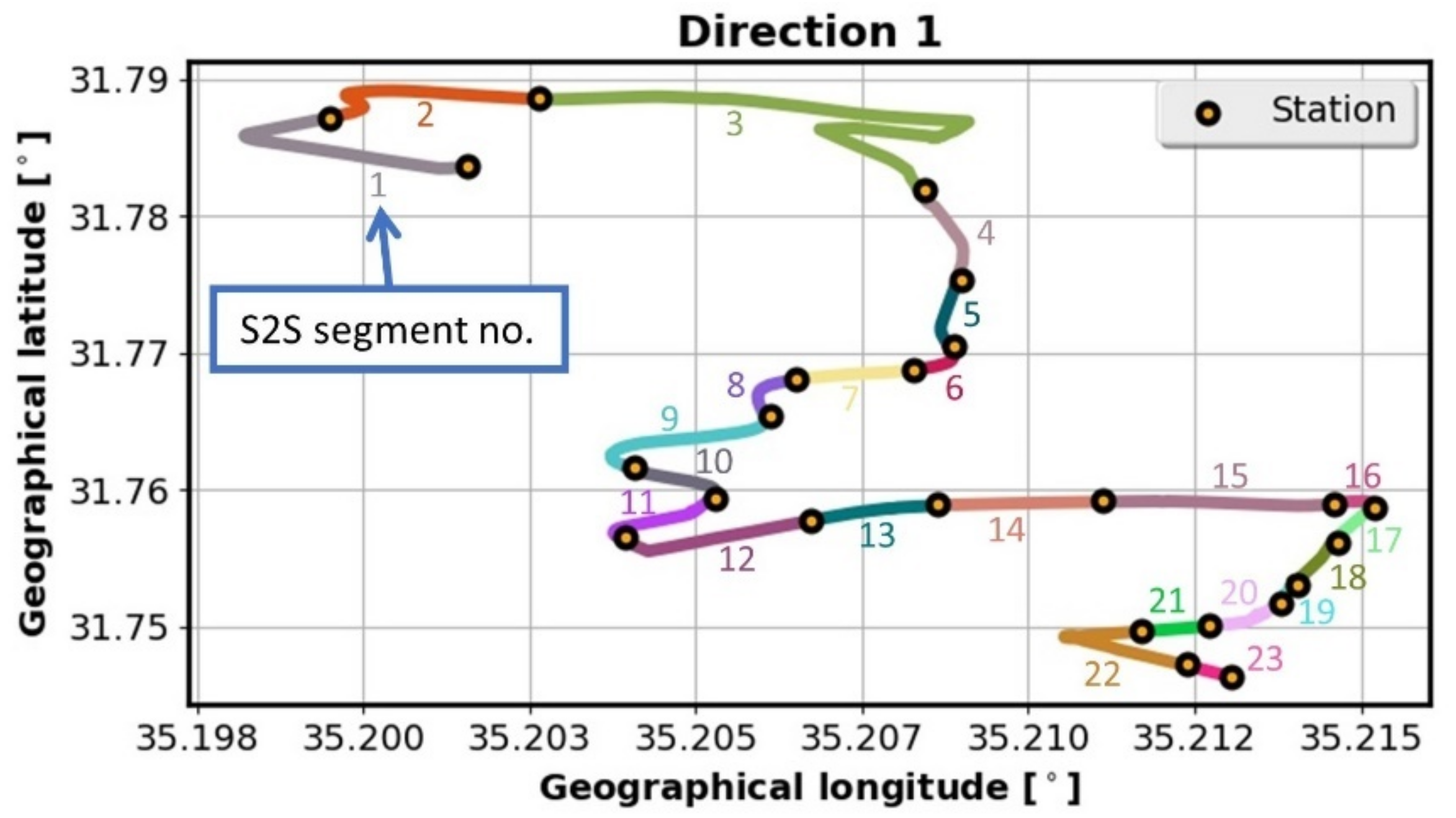
• Information related to bus route(s): reference GPS coordinates of route, station locations, and route timetable.
• LSR GPS tracking data: time series of vehicle geographical coordinates (latitude and longitude), elevation (altitude), velocity, and cumulative distance travelled.

Reference route coordinates facilitated the assignment of the recorded LSR tracking data to corresponding S2S segments. Bus station locations were needed for route segmentation into S2S segments. Vehicle GPS coordinates were used to identify the current S2S segment during the LSR GPS data-mapping process. Altitude data were needed for the reconstruction of the road slope profile along the route [36], which could be fed directly to the fleet microsimulation model. The mapped S2S segment data (Figure 2a) were used to generate the data-driven traffic model described by spatial–temporal maps of (i) mean velocities, (ii) bus-stopping probabilities, and (iii) bus dwell times at stations (Figure 2b). Based on the established traffic model and the known route timetable, a set of HSR synthetic driving cycles was finally generated for each trip by utilizing the Markov-chain-based synthesis method and the reference transport system TPM model (Figure 2c).

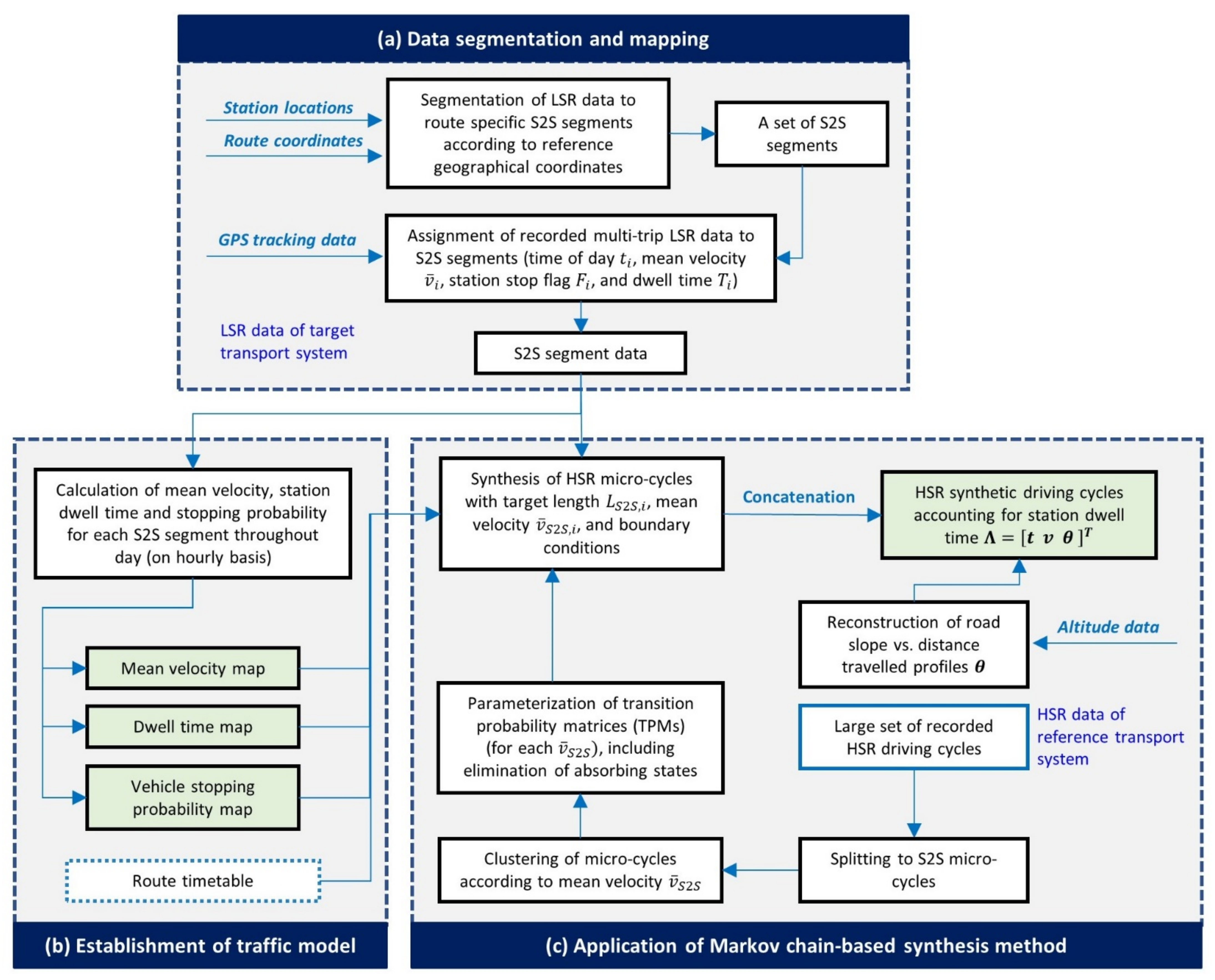
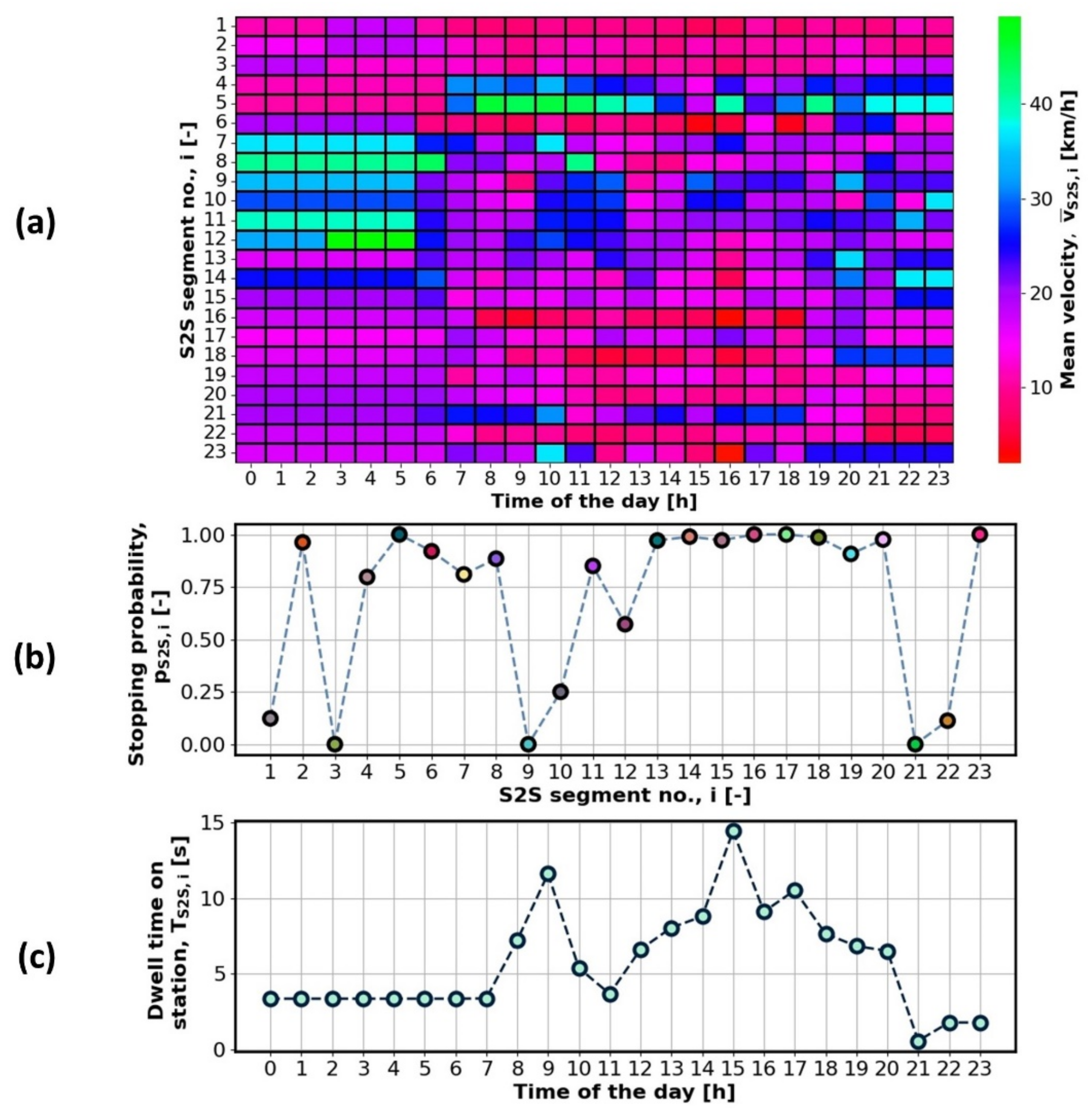
2.4. LSR Data-Supported Traffic Model Generation

A rich set of LSR city bus driving cycles was continuously recorded in the target city over a period of one month. The average GPS sampling time was 40 s (i.e., the average sampling rate was 0.25 Hz). The data considered here correspond to both directions of the single city route shown in Figure 3. Direction 1 included 23 S2S segments, and Direction 2 consisted of 30 S2S segments. The route length was approximately 9 km.

During the one-month recording period, multiple buses (including those from other overlapping routes) traveled over each S2S segment numerous times all over the day. To account for time-varying traffic conditions, the recorded mean velocities of each S2S segment were averaged on an hourly basis. The resulting heat map, shown in Figure 4a for Direction 1, indicates that the average velocities could significantly vary throughout the day (higher velocities in night) and road segments (lower velocities in congested roads).

The stopping probability for each bus station was calculated as:

$$p_{S2S,i} = \frac{n_{stp,i}}{n_{tot,i}},$$

(1)

where $n_{stp,i}$ is the number of stopping occurrences at the ith bus station and $n_{tot,i}$ is the total number of recorded S2S micro-cycles. The resulting map, which was averaged in time and is shown for Direction 1 in Figure 4b, indicates that stopping occurred regularly for certain stations (the probability approaches 1), while it was rare or occasional for other stations.

The time needed for a bus to traverse the ith S2S segment could be estimated from the segment length ($L_{S2S,i}$) and its mean velocity (${\overline{v}}_{S2S,i}$):

$$t_{S2S,i} = \frac{L_{S2S,i}}{{\overline{v}}_{S2S,i}}.$$

(2)

The average dwell time ($t_{dwell}$) at each bus station and for a single recorded driving cycle could then be determined from the actual route traversing time ($t_{drv,real}$) and the cumulative value of S2S segment traversing time ($t_{drv,est}$):

$$t_{dwell} = \frac{t_{drv,real}-t_{drv,est}}{n_{st,stp}} = \frac{t_{drv,real}-{\sum }_{i = 1}^N{t}_{S2S,i}}{n_{st,stp}},$$

(3)

where $n_{st,stp}$ represents the number of stations at which the bus stopped for the considered driving cycle. The individual dwell times, given by Equation (3), were then averaged for each station along the day, on an hourly basis, to map the overall average dwell time $T_{S2S,i}$. The resulting map, shown in Figure 4c, shows that the dwell time $T_{S2S,i}$ increased in the morning and the afternoon commuting hours, which could be explained by higher numbers of passengers entering and exiting buses during these periods.

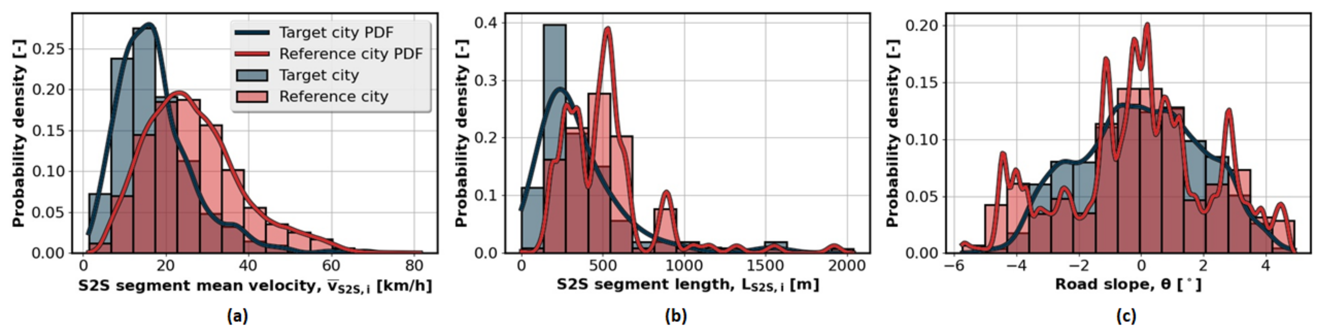
2.5. Comparative Characteristics of Target and Reference City

The comparative distributions of the city bus transport system S2S segment features for the reference city (Dubrovnik) and the target city (Jerusalem) are shown in Figure 5. Although certain differences can be observed between the two sets of distributions (e.g., the mean velocities and the segment lengths are somewhat lower for the target city than the reference city), the distributions are quite similar in shape and values, including very similar road slope features. Therefore, the available city bus HSR driving cycles recorded in the reference city could be used as a basis for generating synthetic HSR driving cycles for the target city.

3. Fundamentals of Markov-Chain-Based Method of Driving Cycles Synthesis

The Markov-chain-based driving cycle synthesis procedure can be divided into three distinctive steps [4,19]: (i) modeling, (ii) generation, and (iii) validation of synthetic driving cycles.

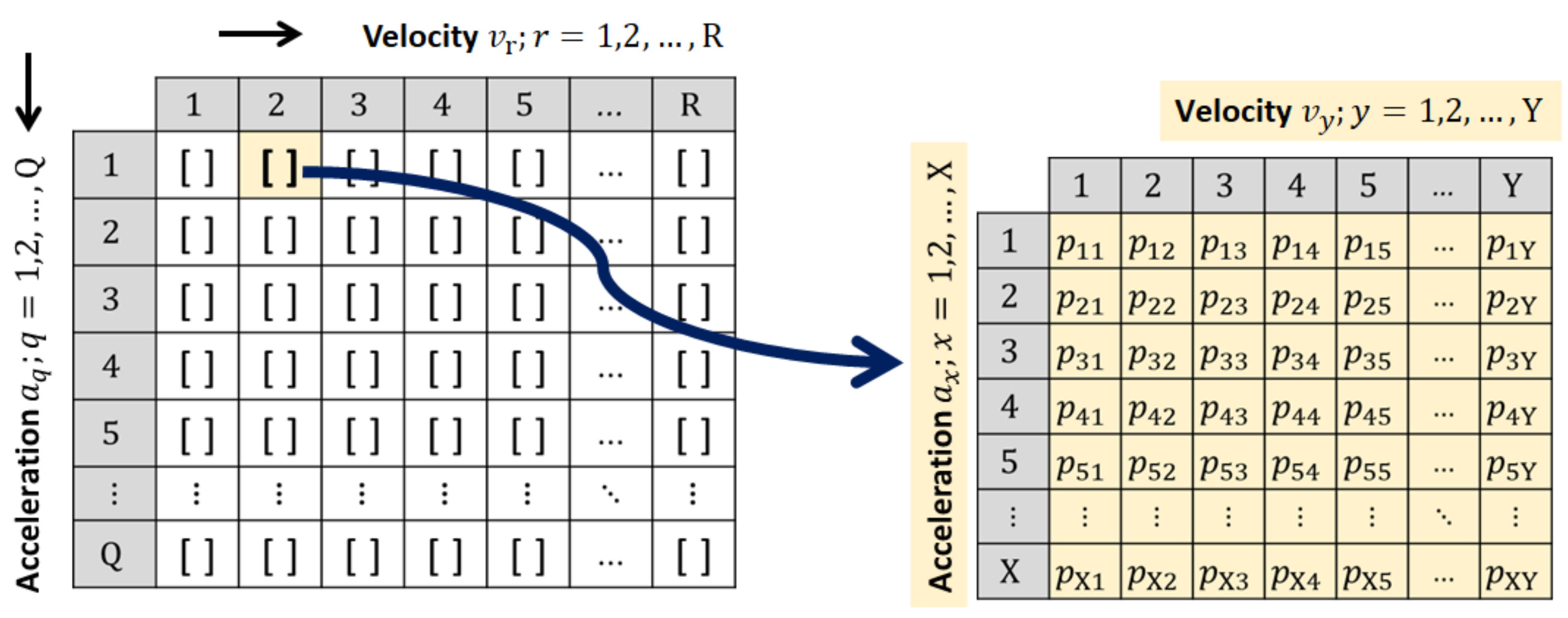
3.1. Modeling of Driving Cycles

A Markov chain is defined as an attainable set of discrete-time states $\left\{X_0,X_1, X_2,\dots \right\}$ of a considered system, for which the following Markov property condition is satisfied at any discrete time step k [37]:

$$P\left(X_{k+1} = s_{k+1}|X_k = s_k,\dots ,X_0 = s_0\right) = P\left(X_{k+1} = s_{k+1}|X_k = s_k\right),$$

(4)

where $s_0,\dots ,s_k, s_{k+1}$ represent exact realizations of the system states and $P\left(X_{k+1} = s_{k+1}|X_k = s_k\right)$ denotes the transition probability from the state $X_k$ to the state $X_{k+1}$. The interpretation of Equation (4) is that the transition of the system to the next state $X_{k+1}$ solely depends on the current state $X_k$, and not on the previous states $X_0,\dots ,X_{k-1}$.

In the context of driving-cycle synthesis, combinations of discrete-amplitude values of vehicle velocity and acceleration are typically used as Markov chain states [19,20,21]. Here, the (city bus) velocity was discretized in the range from 0 to 90 km/h with a resolution of 0.1 km/h (901 discrete values in total) and the acceleration was in the range from −2 to 2 m/s² with a resolution of 0.1 m/s² (41 discrete values in total) [28,34].

The transition probabilities between states are expressed through a four-dimensional (4D) transition probability matrix (TPM; see Figure 6), and they are defined as:

$$p_{qr,xy}≔P\left(X_{k+1} = \left\{a_x,v_y\right\}|X_k = \left\{a_q,v_r\right\}\right).$$

(5)

To determine the TPM from recorded driving cycles, each recorded acceleration–velocity pair is rounded to the nearest discrete Markov chain state. Then, the transitions between states are counted and stored within the TPM; e.g., if the transition from the state $\left\{a_q,v_r\right\}$ to the state $\left\{a_x,v_y\right\}$ is observed, the corresponding element of the TPM is increased by 1. Finally, the number of transitions from each state are scaled (normalized) to have a total sum of 1 according to Equation (6) in order to obtain a proper probability distribution:

$$\sum _x\sum _y{p}_{qr,xy} = 1, \forall q,r.$$

(6)

TPMs are typically implemented in the form of an array (see Figure 6). For very high number of Markov chain states, this could lead to excessive memory requirements and low cycle-generation computational efficiency (in total, 36,941² transition probabilities for the particular study). This problem can be overcome by exploiting the TPM sparsity property, i.e., that it contains many zero elements [20], which is because a lot of state transitions are absent (e.g., high jumps in vehicle velocity between two consecutive steps are impossible). The TPM can thus be implemented in a sparse form based on the dictionary-of-keys data structure [34,38,39], which was applied in this paper. In this notation, ordered tuples are used as dictionary keys to retrieve transition probabilities $P\left(X_{k+1}|X_k\right)$ for a certain state $X_k$. Each tuple representing one Markov state is defined by indices of discrete values of vehicle velocity and acceleration. Non-relevant, zero-probability transitions are avoided in this way.

3.2. Generation of Synthetic Driving Cycles

Synthetic driving cycles are generated by using the TPM and a random number generator. The procedure is known as Monte Carlo Markov Chain (MCMC) method, and it can be described as follows [40]:

▪

In the initial time step ($k = 0$ the vehicle velocity and acceleration states are initialized to arbitrary values (typically to zeros).

▪

Being in the state $X_k = \left\{v_k,a_k\right\}$ the next state $X_{k+1} = \left\{v_{k+1},a_{k+1}\right\}$ is determined by sampling from the distribution $P(X_{k+1}|X_k)$ stored in the TPM by using a random number generator.

▪

The process is iteratively repeated until meeting a terminating condition (e.g., the target time duration or target travelled distance).

3.3. Validation of Synthetic Driving Cycles

Since driving cycle synthesis is based on stochastic modeling and generation, theoretically infinite number of driving cycles can be generated using a single TPM. Therefore, a validation procedure should be employed to select the most representative driving cycle(s), which, in statistical sense, faithfully resemble the recorded driving cycles. This is typically done through comparisons of key statistical features of synthetic and recorded driving cycles, such as mean value and standard deviation of velocity and acceleration (see [19,20,28] for more details).

4. Synthesis of HSR Driving Cycles from LSR Data-Based Traffic Model

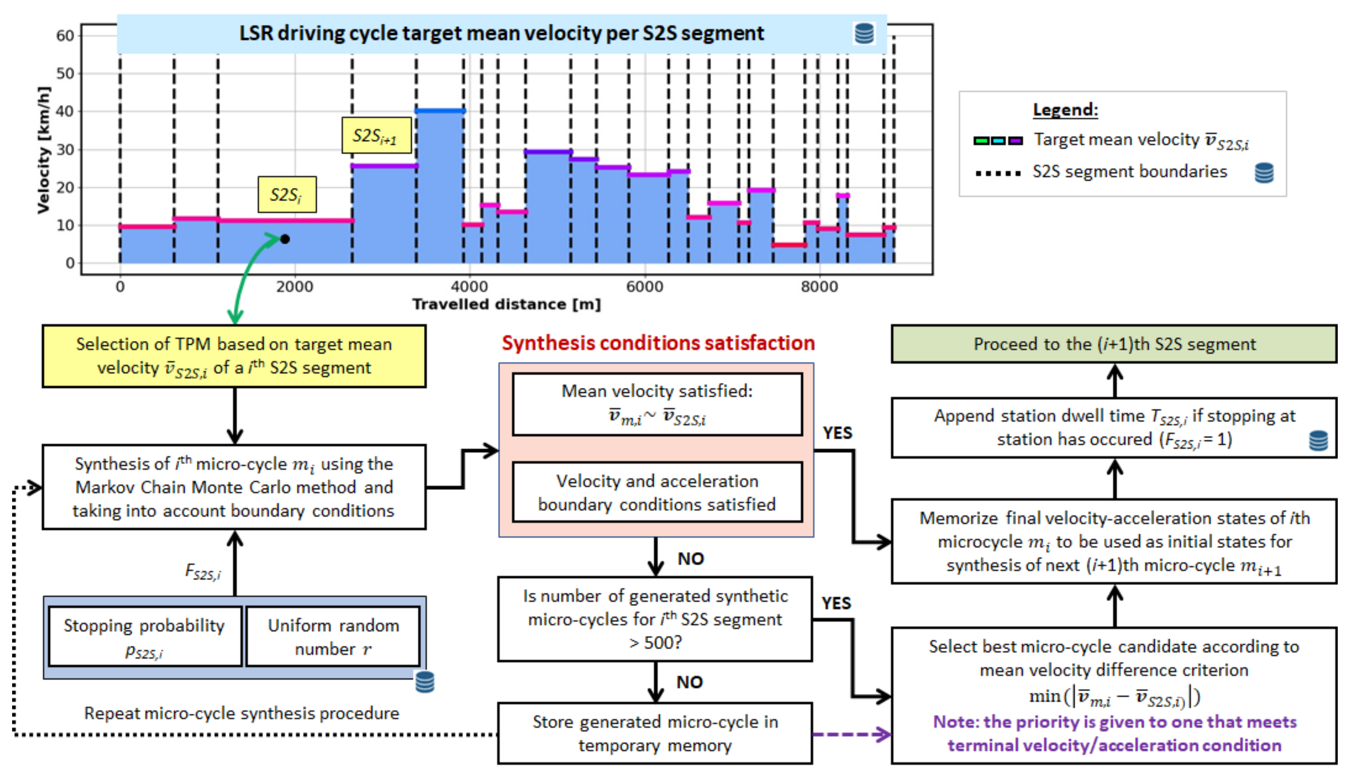
4.1. Procedure of S2S Micro-Cycle Synthesis

The main idea of this method is to iteratively generate HSR micro-cycles for each S2S segment and finally select the representative synthetic micro-cycle. The micro-cycle selection criteria are to closely match the target statistical features represented by the LSR data-gained traffic model for the given S2S segment, which includes (see Figure 4): (i) the mean velocity ${\overline{v}}_{S2S,i}$, (ii) the stopping probability for the segment end-station $p_{S2S,i}$, (iii) the dwell time at the segment end-station $T_{S2S,i}$, and (iv) the segment length (i.e., the travelled distance) $L_{S2S,i}$. The selected micro-cycles, with properly arranged boundary conditions and the dwell time $T_{S2S,i}$ added, are finally concatenated into a full-trip HSR driving cycle.

The micro-cycle synthesis procedure is illustrated in Figure 7, and it can be divided into the following steps:

i.

Clustering the HSR-recorded micro-cycles and determining the corresponding TPMs (Section 4.2).

ii.

Setting the velocity and acceleration initial conditions to match the final conditions of the prior S2S segment micro-cycle, acquiring the target statistical features from the LSR data-based traffic model for the given S2S segment, and selecting the TPM based on the target S2S segment mean velocity.

iii.

Randomly determining if the vehicle should stop at the segment end-station based on the predefined stopping probability $p_{S2S,i}$ as:

$$F_{S2S,i} = \left\{\begin{array}{c}0, r<p_{S2S,i} \\ 1, r\ge p_{S2S,i} \end{array}\right.,\hspace{1em}\hspace{1em}r ~ U\left(0, 1\right),$$

(7)

where $F_{S2S,i}$ is the bus-stopping flag and $r$ is random number sampled from the uniform distribution. If this condition is satisfied, the final condition is set to zero velocity/acceleration; otherwise, the final condition is unspecified/floating.

iv.

Generating synthetic micro-cycle based on the selected TPM and target statistical features including travelled distance and the determined boundary (initial and final) conditions.

v.

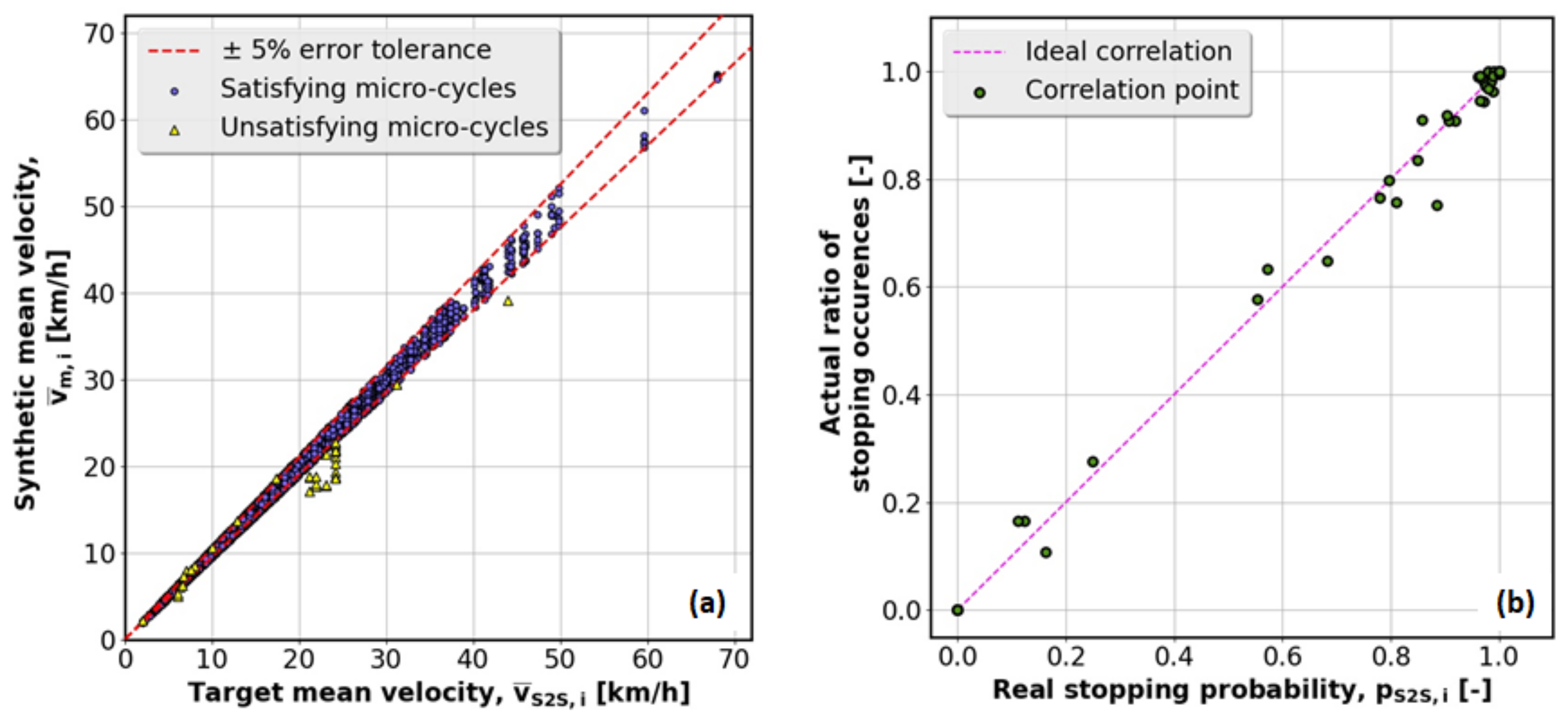
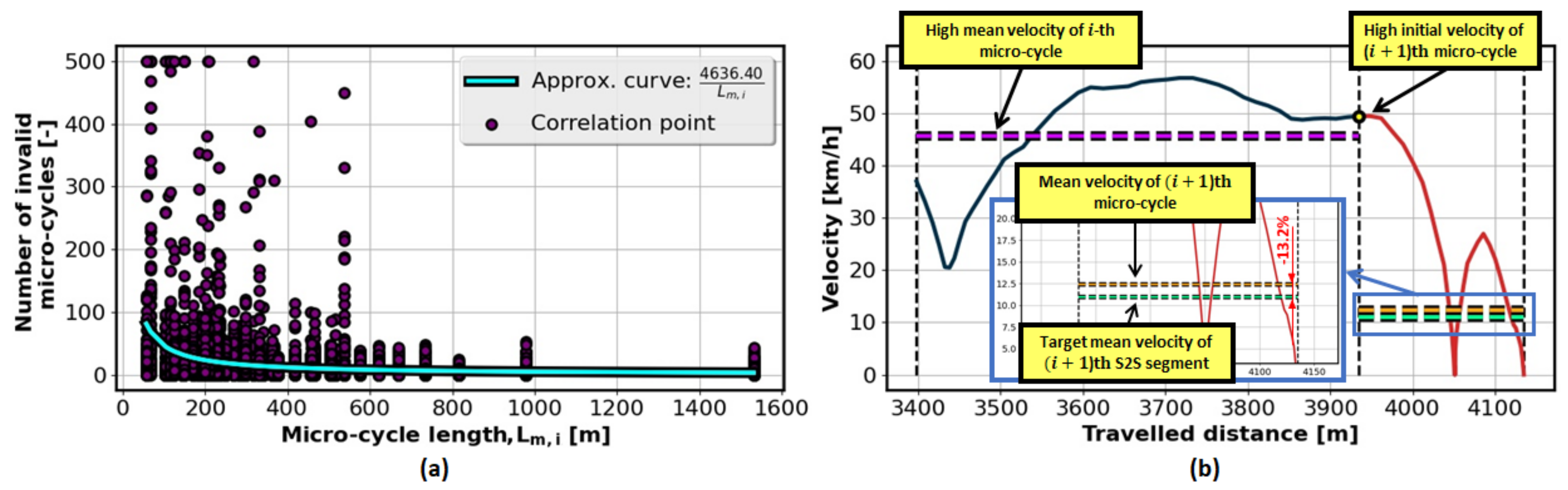
Checking if the target S2S segment mean vehicle velocity is achieved under the specified tolerances (±5%). If the selection condition is satisfied, the generated micro-cycle is adopted. Otherwise, new micro-cycles are iteratively generated and the selection condition is continuously checked. If the selection condition is not satisfied in a pre-defined number of iterations (500 here), the micro-cycle with the mean velocity closest to the target value is selected.

Special emphasis is devoted to the feasibility of overall procedure in terms of matching the final and initial conditions of the consecutive micro-cycles while considering realization features of the TPM including possible absorbing states (see Section 4.4 for more details).

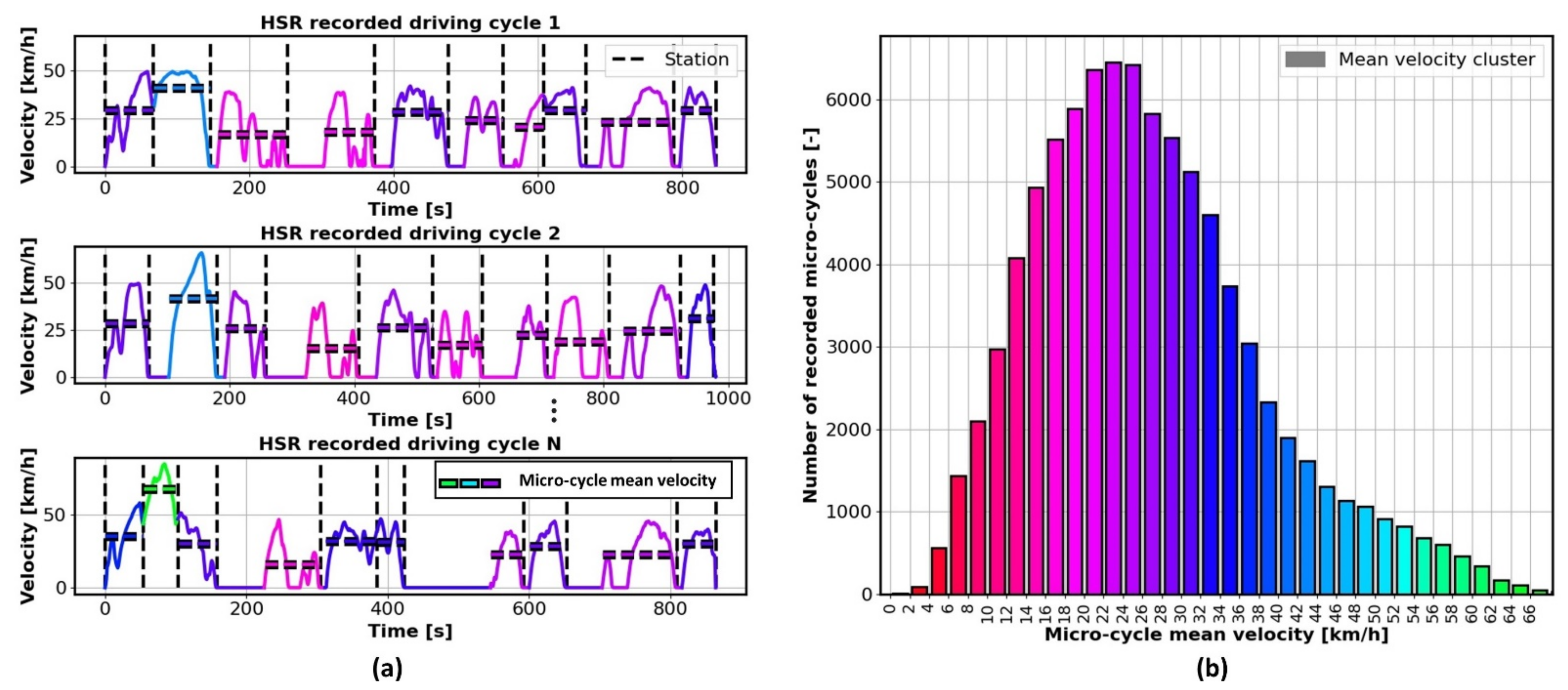
4.2. Clustering of HSR-Recorded Micro-Cycles and Determining Corresponding TPMs

The mean velocities of generated synthetic driving cycles tend to group around the mean value of widely distributed, HSR-recorded velocities (see Figure 7) if a single TPM is used to model the reference transport system. This can lead to an excessively high number of generated micro-cycles until a valid one is selected. In order to make the synthesis procedure numerically more efficient, the recorded HSR micro-cycles in this research were clustered with respect to their mean velocities (see illustration in Figure 8), and an associated TPM was determined for each cluster. The clusters were defined in the range from 0 to 68 km/h, with a width of 2 km/h, thus resulting in 35 clusters and accordingly 35 TPMs in total. As such, the micro-cycle synthesis is based on the TPM that corresponds to the target mean velocity of the current S2S segment. By narrowing the range of recorded micro-cycle mean velocities covered by the TPM model, the number of iterations needed to select the valid micro-cycle could be substantially reduced.

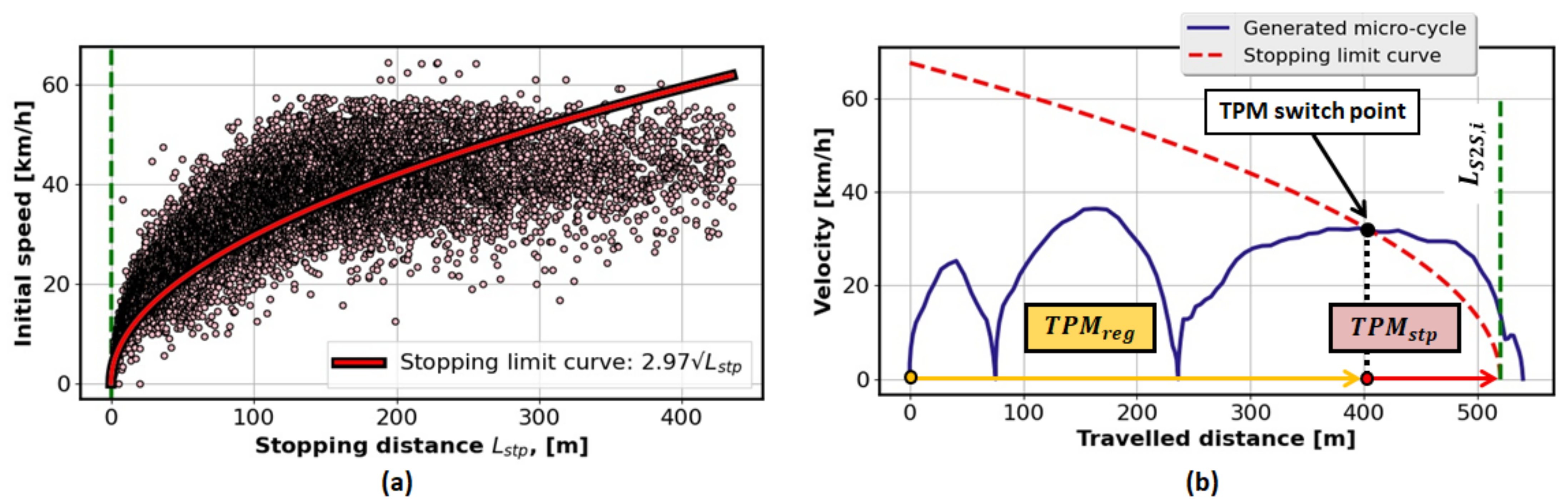
4.3. Accounting for Stopping-Related Final Condition

A bus may or may not stop at the S2S segment end-station depending on condition (7). The micro-cycle synthesis method should cover both of these final condition scenarios. The synthesis is straightforward if the bus does not stop at the station, because the final condition is not imposed in that case. On the other hand, realizing the zero velocity/acceleration final condition in a statistically representative way poses a challenge. To solve this problem, three distinct methods were developed and assessed: (i) using an additional TPM corresponding to end-cycle-stopping data only, (ii) employing a dual TPM reflecting the recorded micro-cycle features in forward-looking and backward-looking senses, and (iii) extending the micro-cycle to satisfy the zero-velocity final condition and compressing the extended micro-cycle to the target length.

4.3.1. Using Additional TPM Related to Stopping Mode

The stopping-mode TPM is extracted from the final-phase data of all recorded micro-cycles that end with the zero-velocity final condition. The final phase is bounded by the stopping start and end points. The stopping start point is determined by counting the individual acceleration samples starting from the (zero-velocity) end point (i.e., backward in time) based on the condition that the ratio of negative/stopping accelerations to all accelerations falls below a predefined threshold (set to 80% here).

To establish a right timing of the transition from regular TPM ($TP{M}_{reg}$) to stopping TPM ($TP{M}_{stp}$) when generating the micro-cycles (Figure 9b), numerous micro-cycles were synthesized based on the stopping TPM for different initial velocities. This resulted in the initial velocity vs. stopping distance plot illustrated by dots in Figure 9a, which was approximated with a constant-deceleration square root function (solid line in Figure 9a). The transition from $TP{M}_{reg}$ to $TP{M}_{stp}$ was set to occur if the current micro-cycle velocity vs. remaining distance point fell below the stopping limit curve (see illustration of this transition in Figure 9b).

It should be noted that the target stopping and, thus, the overall travelled distance could not be guaranteed because of the approximation of stopping limit curve and the stochastic nature of the micro-cycle synthesis method. To overcome this issue, the termination condition of the iterative synthesis procedure (see Figure 7) had to be extended to request that the target distance was satisfied with some error tolerance (set to $\pm$5% here). However, this intervention significantly affected the overall numerical efficiency; for instance, it turned out that only 25% of all generated micro-cycles satisfied the target distance condition. Additionally, the statistical representativeness of the generated micro-cycle was affected by certain ambiguities of determining and activating the stopping TPM.

4.3.2. Using Dual TPMs

The dual TPM method is aimed to generate micro-cycle of the exact/target length in a single step. The first TPM (denoted as FWD TPM) is constructed regularly (Section 3), i.e., by counting transitions between recorded micro-cycle states in the forward-in-time direction. The second TPM (designated as BWD TPM) is determined in the backward manner, i.e., by counting transitions between states backward-in-time (i.e., from the end-station to the start-station of an S2S segment). After normalization, the BWD TPM finally contains the following conditional probability distributions:

$$p_{qr,xy}≔P\left(X_k = \left\{a_x,v_y\right\}|X_{k+1} = \left\{a_q,v_r\right\}\right),$$

(8)

which represents the probability of being in the state $\left\{a_x,v_y\right\}$ in the kth time step if the state in the (k+1)th time step is known and equal to $\left\{a_q,v_r\right\}$. It should be noted that (i) the same set of recorded micro-cycles with the zero-velocity final condition is used for constructing both FWD and BWD TPMs, (ii) both FWD and BWD synthesis results in TPMs that faithfully resemble the real/recorded data, and (iii) synthesizing the BWD micro-cycle with the zero-velocity initial condition and combining it with the FWD one into the final micro-cycle (see Figure 10a) allows for defining the final/merged micro-cycle with the zero-velocity final condition.

In the micro-cycle synthesis step, two micro-cycles of the target length are generated, both having the zero-velocity initial condition: the first one is based on the FWD TPM and evaluates forward in time (from start to end-segment station), while the second one employs the BWD TPM and evaluated backward in time (from end to start-segment station; see Figure 10a for illustration). The FWD and BWD micro-cycles are then combined into a single, final micro-cycle, as illustrated in Figure 10a by the dashed yellow line. The two micro-cycles are merged together in one of their intersection points to provide a smooth velocity transition. Note that there is at least one intersection point due to the zero-velocity initial conditions and positive velocities. When there is more than one intersection point, the intersection point that minimizes the difference in the boundary accelerations of the two micro-cycles is selected as the final micro-cycle merging point (Figure 10b). A certain weakness of this approach is the need of calculating and storing dual TPMs, which leads to computationally less efficient preprocessing and higher memory requirements.

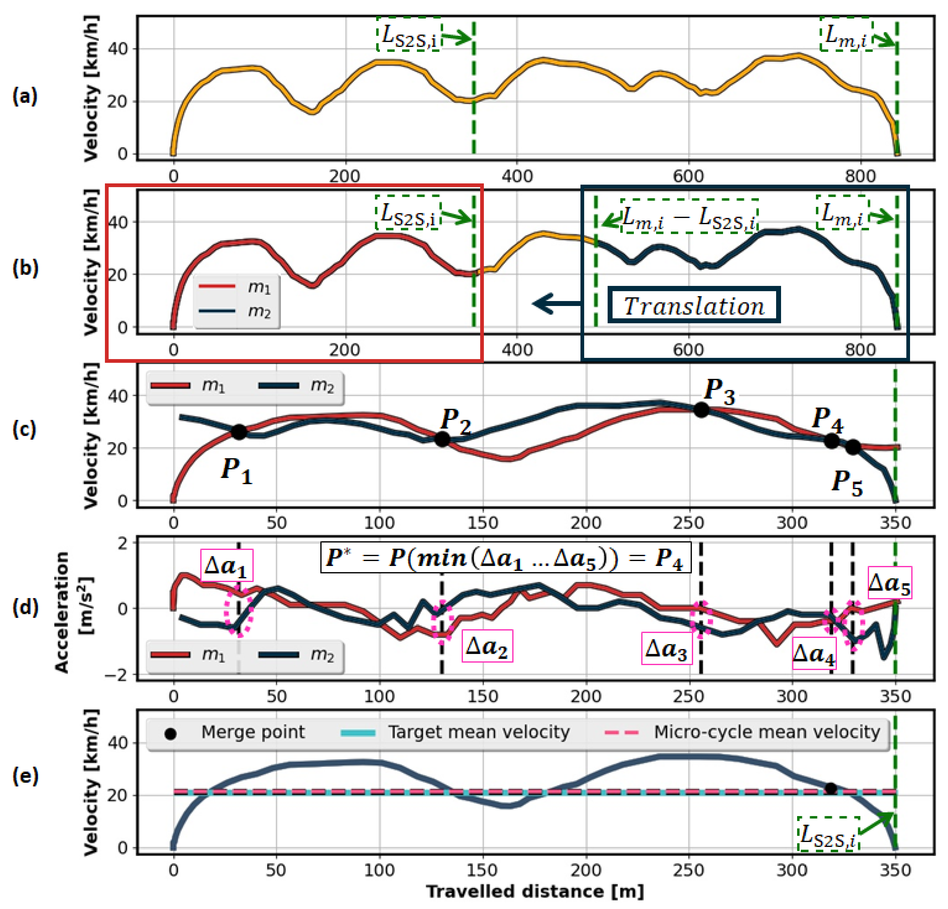
4.3.3. Using Compression of Micro-Cycle Expanded to Stopping

To keep the exactness of the second approach, while avoiding usage of dual TPMs per each cluster, the following third method is proposed. The method is again based on one-step merging of FWD and BWD micro-cycles that are, however, generated by only using the regular FWD TPM. The synthesis procedure is elaborated below based on the illustration in Figure 11:

i.

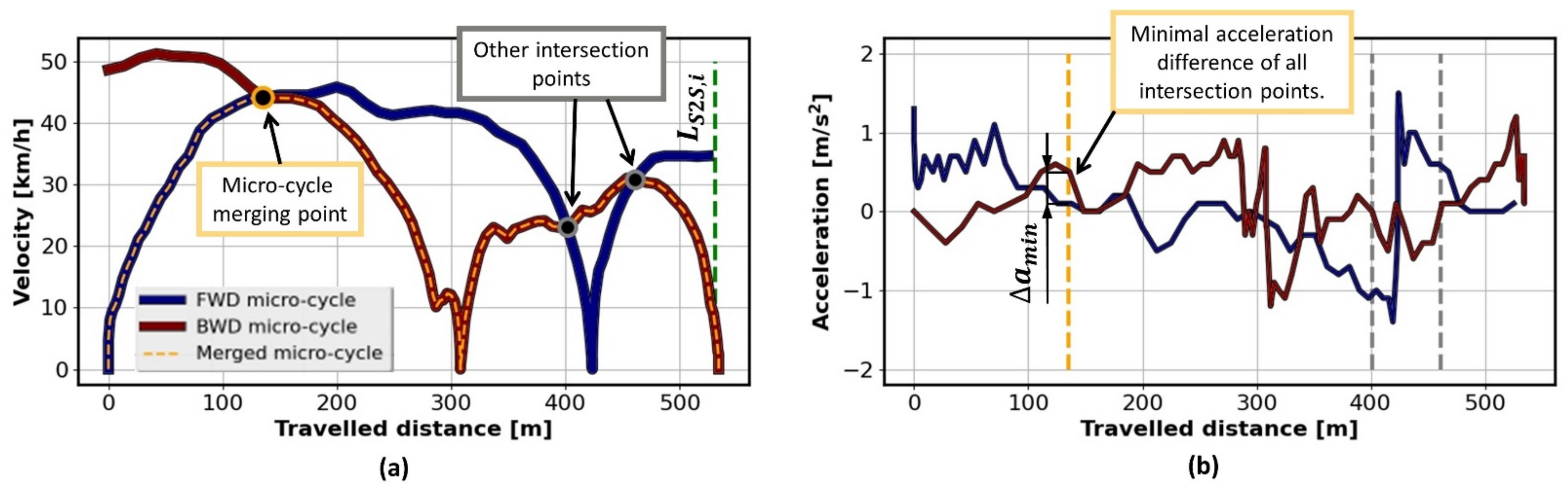
Using the regular TPM to generate a single micro-cycle whose length $L_{m,i}$ is greater or equal than the target length $L_{S2S,i}$ and at the same time corresponds to the minimum length for which the zero-velocity final condition is reached (Figure 11a). It should be noted that only the TPMs corresponding to the range from 0 to 48 km/h can be selected in this procedure, because the recorded driving cycles used for calculating TPMs with mean velocities greater than 48 km/h did not include S2S segment end-station-stopping. Therefore, if the target mean velocity is in the range [50, 68] km/h (see Figure 8b), the TPM corresponding to the mean-velocity range [46, 48] km/h is exceptionally employed in the synthesis process to make it consistent.

ii.

Decomposing the generated micro-cycle into left- and right-end sections, denoted in Figure 11b as $m_1$ and $m_2$, respectively, where both have the length equal to the target length $L_{S2S,i}$.

iii.

Translating the right-end section $m_2$ in the backward direction to become aligned with the left-end section $m_1$ in terms of equal lengths corresponding to the target length (see Figure 11c and note that the initially longer micro-cycle length in Figure 11a is now compressed to the target length).

iv.

Detecting intersection points ($P_1,P_2,\dots ,P_n$) of the aligned velocity vs. distance profiles $m_1$ and $m_2$ (Figure 11c).

v.

Determining the merging point P* as the one that minimizes the acceleration bump between the profiles $m_1$ and $m_2$ (see illustration in Figure 11d, showing that $P^{*} = P_4$ is the merging point).

vi.

Merging the profiles $m_1$ and $m_2$ in the intersection point $P^{*}$ to obtain the final, single micro-cycle (Figure 11e).

4.3.4. Brief Comparative Assessment and Recommendation

As discussed in Section 4.3.1, the first approach is based on approximation of vehicle-stopping model and its activation in the final stage of micro-cycle synthesis. As such, it suffers from an inaccuracy of synthetic micro-cycle features with emphasis on its length or computational inefficiency when the condition on micro-cycle length is “artificially” imposed.

On the other hand, the second and third approaches are exact because they realize the zero-velocity final condition by evaluating an extra micro-cycle in the backward-in-time direction with the zero-velocity initial condition. The weakness of the second approach is that generating the extra micro-cycle requires the corresponding extra TPM model, thus affecting modeling computational efficiency and memory requirements. The third approach does not share this weakness, as it does not rely on dual TPM model but rather expands the forward-in-time micro-cycle generation until the zero-velocity final condition is met.

However, potential drawbacks of the third method include the necessity for long micro-cycle generation until reaching the stopping final condition ($L_{m,i}\gg L_{S2S,i}$ in Figure 11a) and discarding the high-mean-velocity TPM models (Section 4.3.3). This is deemed to be of lesser concern compared to the excessive memory requirement of the second, dual TPM-based method. Hence, the third approach was adopted for further consideration in this paper and is generally recommended. However, the second approach is a very competitive alternative, and it is up to the designer to decide which one would better suit a particular application.

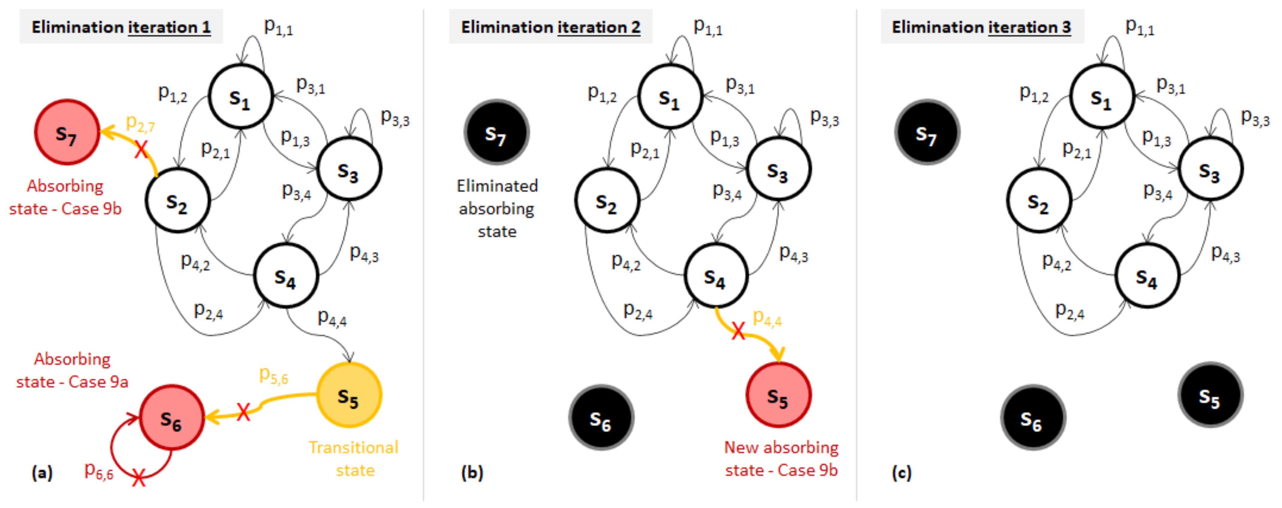
4.4. Ensuring Feasibility of Micro-Cycle Synthesis Procedure

As described in Section 4.2, the synthesis of consecutive micro-cycles over a sequence of S2S segments is based on multiple TPMs, which are determined from different sets of HSR-recorded micro-cycles depending on their mean velocity. Each TPM possesses unique combinations of velocity-acceleration states, as well as transition probabilities between them. Consequently, the multi-TPM synthesis approach can cause the stopping of micro-cycle generation in cases when the velocity-acceleration state at the end of an ith micro-cycle is not present in the TPM of the following (i+1)th micro-cycle for the proper realization of the boundary condition (i.e., providing that the initial condition of (i+1)th micro-cycle is equal to the final condition of the ith micro-cycle). In order to prevent the stalling of the micro-cycle generation procedure, an additional boundary condition was introduced to be satisfied (see the 2nd condition in the orange-shaded box of Figure 7), i.e., it is checked if the final velocity-acceleration state of the ith micro-cycle is included in the TPM of the (i+1)th micro-cycle. If this boundary condition is not satisfied, the iterative process of generating new micro-cycles is continued, as shown in Figure 7.

The multi-TPM-based micro-cycle generation procedure can also stall if a so-called absorbing state of the TPM is reached (see Figure 12 for graphical illustration of absorbing Markov chain example). The absorbing state is defined as the state without transition to any other state, i.e., the state for which one of the following two conditions holds [41]:

$$P\left(X_{k+1} = s_{k+1}|X_k = s_k\right) = 1, \forall s_{k+1} = s_k, \mathrm{or}$$

(9a)

$$\left(X_{k+1} = s_{k+1}|X_k = s_k\right) = 0, \forall s_{k+1}.$$

(9b)

For instance, the absorbing states could appear if the final state of a recorded micro-cycle appears one or eventually more times as the sequence of the same state (Case (9a)) or as the individual state (Case (9b)) among all states/samples of the recorded micro-cycles from a single mean velocity cluster that are used for calculating the single-cluster TPM. Therefore, it is necessary to detect and eliminate the absorbing states. The elimination procedure applied to each TPM is described as follows (Figure 12):

• Iterate through all TPM states, detect all absorbing states based on conditions (9a) and (9b), and set their transition probabilities to zero (see states and transition probabilities highlighted in red in Figure 12a).
• Find all TPM states that directly lead to the absorbing states detected in Point 1 (see transition probabilities highlighted in orange in Figure 12a).
• Set the TPM probabilities corresponding to the transitions from the states detected in Point 2 to the absorbing states from Point 1 to zero (see “X” marks in Figure 12a).
• If the transitional states found in Point 2 are such that they lead only to absorbing states detected in Point 1 (see state highlighted in orange in Figure 12a), then declare these transitional states as the absorbing ones (Figure 12b) and apply the elimination steps defined by Points 1-3 to them, as well.
• Re-normalize the corrected TPM (Figure 12c) to satisfy condition (6).

5. Validation of Proposed Micro-Cycle-Based Synthesis Method

For the considered single-route, full-month case study (Section 2), a total of 5777 HSR micro-cycles concatenated into 218 full-trip driving cycles were generated for both route directions by using the synthesis method presented in Section 4. In order to validate the generated driving cycles and the synthesis method itself, the generated synthetic micro-cycles were analyzed, as discussed below, with emphasis on mean velocity replication accuracy and numerical efficiency. The micro-cycle target length and final conditions were explicitly satisfied, so they were omitted from the numerical analysis.

Figure 13 shows examples of two synthetic driving cycles in each direction. Visual inspection indicates that the generated driving cycles followed the S2S segment target velocities, which varied along the day based on the traffic model shown in Figure 4a. Similarly, the S2S segment end-station-stopping outcome could vary along the day (e.g., stopping occurred for the end-station of 12th segment for Driving cycle 1 but not for Driving cycle 2) because the stopping flag was randomly generated based on the stopping probability model shown in Figure 4b and Equation (7).

The mean velocity replication accuracy is assessed based on the relative residual metrics given by:

$$\epsilon = \frac{{\bar{v}}_{S2S,i}-{\bar{v}}_{m,i}}{{\bar{v}}_{S2S,i}}·100\%,$$

(10)

where ${\bar{v}}_{S2S,i}$ and ${\bar{v}}_{m,i}$ denote the target and actual micro-cycle mean velocity, respectively. The results shown in

Table 1. Micro-cycle mean velocity validation statistics.

Mean Velocity Condition	Total Number	Relative Mean Velocity Residual Statistics, ε [%]
		Min	Median	Mean	Max	Std
Satisfied	5740 (99.4%)	−5.0	0.28	0.19	5.0	2.9
Unsatisfied	37 (0.64%)	−13.3	9.8	8.7	23.3	10.6

illustrate that a great majority of generated micro-cycles (i.e., 99.4% of them) satisfied the mean velocity matching condition $\left|\epsilon \right|<5\%$ (Section 4). The remaining micro-cycles corresponded to the case when the maximum number of iterations (500 here) was reached. The residuals of those very rare micro-cycles could still be considered relatively small (up to 23%). The graphical visualization of the above results is presented in Figure 14a. Figure 14b illustrates that the actual share of stopping outcome closely followed the target-stopping probabilities given in Figure 4b, where certain discrepancies can be explained by the stochastic nature of stopping determination based on Equation (7).

The numerical efficiency was analyzed in terms of the number of micro-cycles needed to be synthesized until obtaining the valid one, i.e., the one which satisfied the prescribed mean velocity and boundary conditions (see Figure 7 and Section 4 for details). The results given in

Table 2. Basic statistics of number of invalid micro-cycles needed to be generated to obtain valid micro-cycle.

Case	Number of Generated Invalid Micro-Cycles per Single Valid Micro-Cycle
	Min	Median	Mean	Max	Std
Stopping applies (3982 valid cycles in total)	0	7	17.1	500	46.1
Stopping does not apply (1795 valid cycles in total)	0	8	20.7	500	53.5
In total	0	7	18.3	500	48.6

indicate that, on average, 18.3 invalid micro-cycles were needed to generate a valid micro-cycle. This ratio was larger for non-stopping micro-cycles (20.7) compared to stopping ones (17.1). This was because the boundary conditions, related to the existence of the ith micro-cycle final state in the (i+1)th micro-cycle TPM, were exclusively applied to non-stopping micro-cycles (Section 4). However, the main cause for micro-cycle invalidity was violating the mean-velocity condition. This is directly illustrated by the data in

Table 3. Further statistics of valid and invalid generated micro-cycles given for individual synthesis conditions.

Case	Total Number of Generated Micro-Cycles
	Valid	Not Valid			Total
		Mean Velocity Condition	Velocity/Acceleration Boundary Condition	Combined Conditions
Stopping applies	3982 (5.5%)	68,228 (94.5%)	0	0	72,210
Stopping does not apply	1795 (4.6%)	35,061 (89.9%)	199 (0.5%)	1950 (5.0%)	39,005
In total	5777 (5.2%)	103,289 (92.9%)	199 (0.2%)	1950 (1.8%)	111,215

, which indicate that from 90 to 95% of all generated micro-cycles were invalid due to mean-velocity condition violation.

The number of generated invalid micro-cycles per a single valid micro-cycle is plotted in Figure 15a with respect to target micro-cycle length. Evidently, the lower the micro-cycle length, the higher the number of invalid micro-cycles. This phenomenon can be explained by the fact that for an initial micro-cycle velocity, which differs greatly from the target mean velocity, reaching the target mean velocity could be very improbable or even impossible for a small micro-cycle length (see Figure 15b for illustration).

The total execution time $T_{exec,tot}$ required to generate all 5777 valid synthetic micro-cycles was 201 s. The execution time $T_{exec}$ required to generate a single micro-cycle had a mean value of 35 ms (

Table 4. Basic statistics of micro-cycle synthesis execution time.

Case	Execution Time, ${\mathit{T}}_{\mathit{e}\mathit{x}\mathit{e}\mathit{c}}$* [ms]
	Min	Median	Mean	Max	Std
Stopping applies	3.9	32.9	50.0	237.5	49.2
Stopping does not apply	0.3	3.8	6.3	37.89	6.8
In total	0.3	15.1	35.4	237.5	45.3

* The computations were performed on a Dell Inspiron 5593 Notebook equipped with 8 GB RAM and an Intel(R) Core(TM) i7-1065G7 CPU @ 1.30 GHz and executed in a Linux Ubuntu 20.04 environment.

), with significant variations due to the varying number of synthesis iterations needed to generate the valid micro-cycle. The execution time was by an order of magnitude higher for the station-stopping case, apparently because of computational overhead related to micro-cycle expansion and compression applied in that case (see Figure 11).

6. Conclusions

The paper presents a Markov-chain-based method for the synthesis of high-sampling-rate (HSR) driving cycles that satisfy statistical features extracted from low-sampling-rate (LSR) vehicle-tracking data over trip segments (e.g., city bus station-to-station segments). These statistical features include: (i) the road segment length and spatial–temporal maps of segment (ii) mean velocity, (iii) station-stopping probability, and (iv) station dwell time. To make the synthesis method representative and numerically efficient, HSR data recorded in a separate reference transport system (i.e., city) were used to build mean velocity-dependent, multiple transition probability matrices (TPMs) for the Markov-chain-trip-segment-based micro-cycle-synthesis.

For a segment end-station-stopping scenario, it is necessary to ensure that the synthetic micro-cycle ends with zero velocity and acceleration and achieve the target length in the single synthesis step if possible. For this purpose, a method based on expanding the synthetic micro-cycle toward the zero final velocity and compressing it to the target length was proposed. On the other hand, to make the synthesis feasible for the station non-stopping scenario, the micro-cycle final state was set to exist within the TPM of the forthcoming micro-cycle and the so-called absorbing states were eliminated from all TPMs. Once the micro-cycles with proper boundary (i.e., initial and final) conditions could be generated, they could be readily expanded with the station dwell time and concatenated into the full-trip synthetic driving cycle.

The proposed HSR driving cycle synthesis method was validated against the LSR recorded data in terms of micro-cycle mean velocity and stopping probability. It was demonstrated that the synthetic and recorded micro-cycles’ features matched each other under the prescribed tolerance and a rather low execution time. Therefore, a large set of realistic HSR synthetic driving cycles can be generated in a numerically efficient way to faithfully characterize a transport system features represented by LSR tracking data. As such, the synthetic driving cycles can conveniently be used in various vehicle-model-based energy-consumption prediction studies.

The main directions of future research should be related to the direct experimental validation of the proposed HSR driving cycle synthesis method. This could be achieved in two distinct ways: (i) by comparing the synthetic and recorded HSR driving cycles for the target city in terms of various relevant statistical features of driving cycles, such as those considered in [34]; and (ii) by comparing predicted and recorded vehicle energy-consumption rates, where the former is based on synthetic driving cycles and experimentally validated vehicle models. The accuracy of approach (iii) should be compared with a trip-based vehicle energy-consumption prediction utilizing a regression model fed by the LSR driving cycle features as inputs. Once the above-mentioned validation tool is established, it would be possible to quantitatively analyze the inaccuracies caused by differences between the reference and target city HSR driving cycle features. Additionally, what extent the prediction accuracy would be improved if the driving cycle validation criteria included the LSR data segment velocity deviation in addition to its mean value could be analyzed.

References

1. European Commission. Available online: https://ec.europa.eu/clima/policies/strategies/2050_en (accessed on 22 April 2022).
2. Carlson, R.; Lohse-Busch, H.; Duoba, M.; Shidore, N. Drive Cycle Fuel Consumption Variability of Plug-In Hybrid Electric Vehicles due to Aggressive Driving; SAE Technical Paper 2009-01-1335; SAE World Congress: Detroit, MI, USA, 2009. [Google Scholar]
3. Fontaras, G.; Franco, V.; Dilara, P.; Martini, G.; Manfredi, U. Development and Review of Euro 5 Passenger Car Emission Factors Based on Experimental Results Over Various Driving Cycles. Sci. Total Environ. 2014, 468, 1034–1042. [Google Scholar] [CrossRef] [PubMed]
4. Giakoumis, E.G. Driving and Engine Cycles; Springer: Cham, Switzerland, 2017; pp. 1–63. [Google Scholar]
5. Barlow, T.; Latham, S.; Mccrae, I.; Boulter, P. A Reference Book of Driving Cycles for Use in the Measurement of Road Vehicle Emissions. In TRL Published Project Report; Transport Research Laboratory: Wokingham, UK, 2009. [Google Scholar]
6. Huertas, J.I.; Giraldo, M.; Quirama, L.F.; Díaz, J. Driving Cycles Based on Fuel Consumption. Energies 2018, 11, 3064. [Google Scholar] [CrossRef] [Green Version]
7. Andrade, G.M.S.D.; Araújo, F.W.C.D.; Santos, M.P.M.D.N.; Magnani, F.S. Standardized Comparison of 40 Local Driving Cycles: Energy and Kinematics. Energies 2020, 13, 5434. [Google Scholar] [CrossRef]
8. Rajan, B.V.P.; McGordon, A.; Jennings, P.A. An Investigation on the Effect of Driver Style and Driving Events on Energy Demand of a PHEV. World Electr. Veh. J. 2012, 5, 173–181. [Google Scholar] [CrossRef] [Green Version]
9. Shankar, R.; Marco, J.; Assadian, F. The Novel Application of Optimization and Charge Blended Energy Management Control for Component Downsizing within a Plug-in Hybrid Electric Vehicle. Energies 2012, 5, 4892–4923. [Google Scholar] [CrossRef]
10. Geller, B.M.; Bradley, T.H. Analyzing Drive Cycles for Hybrid Electric Vehicle Simulation and Optimization. J. Mech. Des. 2015, 137, 041401. [Google Scholar] [CrossRef]
11. Brady, J.; O’Mahony, M. Development of a driving cycle to evaluate the energy economy of electric vehicles in urban areas. Appl. Energy 2016, 177, 165–178. [Google Scholar] [CrossRef]
12. Patil, C.; Naghshtabrizi, P.; Verma, R.; Tang, Z.; Smith, K.; Shi, Y. Optimal battery utilization over lifetime for parallel hybrid electric vehicle to maximize fuel economy. In Proceedings of the American Control Conference, Boston, MA, USA, 6–8 July 2016. [Google Scholar]
13. Naranjo, W.; Camargo, L.E.M.; Pereda, J.E.; Cortes, C. Design of Electric Buses of Rapid Transit Using Hybrid Energy Storage and Local Traffic Parameters. IEEE Trans. Veh. Technol. 2017, 66, 5551–5563. [Google Scholar] [CrossRef]
14. Zhang, F.; Guo, F.; Huang, H. A Study of Driving Cycle for Electric Special-purpose Vehicle in Beijing. Energy Procedia 2017, 105, 4884–4889. [Google Scholar] [CrossRef]
15. Borlaug, B.; Holden, J.; Wood, E.; Lee, B.; Fink, J.; Agnew, S.; Lustbader, J. Estimating region-specific fuel economy in the United States from real-world driving cycles. Transp. Res. Part D Transp. Environ. 2020, 86, 102448. [Google Scholar] [CrossRef]
16. Lee, H.; Lee, K. Comparative Evaluation of the Effect of Vehicle Parameters on Fuel Consumption under NEDC and WLTP. Energies 2020, 13, 4245. [Google Scholar] [CrossRef]
17. Cubito, C.; Millo, F.; Boccardo, G.; Di Pierro, G.; Ciuffo, B.; Fontaras, G.; Serra, S.; Otura Garcia, M.; Trentadue, G. Impact of Different Driving Cycles and Operating Conditions on CO2 Emissions and Energy Management Strategies of a Euro-6 Hybrid Electric Vehicle. Energies 2017, 10, 1590. [Google Scholar] [CrossRef]
18. Fontaras, G.; Zacharof, N.G.; Ciuffoo, B. Fuel consumption and CO2 emissions from passenger cars in Europe—Laboratory versus real-world emissions. Prog. Energy Combust. Sci. 2017, 60, 97–131. [Google Scholar] [CrossRef]
19. Lee, T.K.; Filipi, Z.S. Synthesis of real-world driving cycles using stochastic process and statistical methodology. Int. J. Veh. Des. 2011, 57, 17–36. [Google Scholar] [CrossRef]
20. Škugor, B.; Deur, J. Delivery vehicle fleet data collection, analysis and naturalistic driving cycles synthesis. Int. J. Innov. Sustain. Dev. 2016, 10, 19–39. [Google Scholar] [CrossRef]
21. Liessner, R.; Dietermann, A.M.; Bäker, B.; Lüpkes, K. Derivation of real-world driving cycles corresponding to traffic situation and driving style on the basis of Markov models and cluster analyses. In Proceedings of the 6th Hybrid and Electric Vehicles Conference, London, UK, 2–3 November 2016. [Google Scholar]
22. Esser, A.; Zeller, M.; Foulard, S.; Rinderknecht, S. Stochastic Synthesis of Representative and Multidimensional Driving Cycles. SAE Int. J. Alt. Power. 2018, 7, 263–272. [Google Scholar] [CrossRef]
23. Peng, J.; Jiang, J.; Ding, F.; Tan, H. Development of Driving Cycle Construction for Hybrid Electric Bus: A Case Study in Zhengzhou, China. Sustainability 2020, 12, 7188. [Google Scholar] [CrossRef]
24. Zeyu, C.; Qing, Z.; Jiahuan, L.; Jiangman, B. Optimization-based method to develop practical driving cycle for application in electric vehicle power management: A case study in Shenyang, China. Energy 2019, 186, 115766. [Google Scholar]
25. Ho, S.; Wong, Y.; Chang, V.W. Developing Singapore Driving Cycle for passenger cars to estimate fuel consumption and vehicular emissions. Atmos. Environ. 2014, 97, 353–362. [Google Scholar] [CrossRef]
26. Hereijgers, K.; Silvas, E.; Hofman, T.; Steinbuch, M. Effects of using Synthesized Driving Cycles on Vehicle Fuel Consumption. IFAC Pap. 2017, 50, 7505–7510. [Google Scholar] [CrossRef]
27. Lee, T.K.; Filipi, Z. Real-World Driving Pattern Recognition for Adaptive HEV Supervisory Control: Based on Representative Driving Cycles in Midwestern US; SAE Technical Paper 2012-01-1020; SAE World Congress: Detroit, MI, USA, 2012. [Google Scholar]
28. Topić, J.; Škugor, B.; Deur, J. Synthesis and Validation of Multidimensional Driving Cycles. SAE Int. J. Adv. Curr. Prac. Mobil. 2021, 3, 1558–1568. [Google Scholar]
29. Topić, J.; Soldo, J.; Maletić, F.; Škugor, B.; Deur, J. Virtual Simulation of Electric Bus Fleets for City Bus Transport Electrification Planning. Energies 2020, 13, 3410. [Google Scholar] [CrossRef]
30. Gao, D.W.; Mi, C.; Emadi, A. Modeling and Simulation of Electric and Hybrid Vehicles. Proc. IEEE 2007, 95, 729–745. [Google Scholar] [CrossRef]
31. Zacepins, A.; Kalnins, E.; Kviesis, A.; Komasilovs, V. Usage of GPS Data for Real-time Public Transport Location Visualisation. In Proceedings of the 5th International Conference on Vehicle Technology and Intelligent Transport Systems, Crete, Greece, 3–5 May 2019. [Google Scholar]
32. Silvas, E.; Hereijgers, K.; Peng, H.; Hofman, T.; Steinbuch, M. Synthesis of Realistic Driving Cycles with High Accuracy and Computational Speed, Including Slope Information. IEEE Trans. Veh. Technol. 2016, 65, 4118–4128. [Google Scholar] [CrossRef]
33. Liu, Z.; Ivanco, A.; Filipi, Z.S. Naturalistic driving cycle synthesis by Markov chain of different orders. Int. J. Powertrains 2018, 6, 307–322. [Google Scholar] [CrossRef]
34. Topić, J.; Škugor, B.; Deur, J. Synthesis and Feature Selection-Supported Validation of Multidimensional Driving Cycles. Sustainability 2021, 13, 4704. [Google Scholar] [CrossRef]
35. Erdelić, T.; Carić, T. A Survey on the Electric Vehicle Routing Problem: Variants and Solution Approaches. J. Adv. Transp. 2019, 2019, 5075671. [Google Scholar] [CrossRef]
36. Škugor, B.; Hrgetić, M.; Deur, J. GPS measurement-based road slope reconstruction with application to electric vehicle simulation and analysis. In Proceedings of the 8th Conference on Sustainable Development of Energy, Water and Environment Systems (SDEWES), Dubrovnik, Croatia, 27 September–2 October 2015. [Google Scholar]
37. Gagniuc, P.A. Building the Stochastic Matrix. In Markov Chains: From Theory to Implementation and Experimentation, 1st ed.; John Wiley & Sons: New York, NY, USA, 2017; pp. 25–37. [Google Scholar]
38. Topić, J.; Škugor, B.; Deur, J. Analysis of City Bus Driving Cycle Features for the Purpose of Multidimensional Driving Cycle Synthesis; SAE Technical Paper No. 2020-01-1288; SAE World Congress: Detroit, MI, USA, 2020. [Google Scholar]
39. Topić, J.; Škugor, B.; Deur, J. Analysis of Markov Chain-based Methods for Synthesis of Driving Cycles of Different Dimensionality. In Proceedings of the 23rd IEEE International Conference on Intelligent Transportation Systems, Rhodes, Greece, 20–23 September 2020; pp. 893–900. [Google Scholar]
40. Gamerman, D.; Lopes, H.F. Markov chains. In Markov Chain Monte Carlo: Stochastic Simulation for Bayesian Inference, 2nd ed.; Chapman & Hall/CRC: London, UK, 2006; pp. 113–136. [Google Scholar]
41. Privault, N. Discrete-Time Markov Chains. In Understanding Markov Chains; Springer: Singapore, 2018; pp. 89–113. [Google Scholar]
Figure 1. High-level concept of Markov-chain-based method for generating high-sampling-rate (HSR) synthetic driving cycles with predetermined statistical features extracted from low-sampling-rate (LSR) driving cycle database.
Energies 15 04108 g001
Figure 2. Procedure for converting LSR driving data into HSR synthetic driving cycles including: (a) route segmentation into S2S segments and mapping of recorded GPS tracking data to each S2S segment; (b) establishment of a data–driven traffic model based on spatial–temporal mean velocity, station dwell time and vehicle-stopping probability maps; and (c) generation of HSR synthetic driving cycles with target statistical features based on proposed Markov chain synthesis method.
Energies 15 04108 g002
Figure 3. Geographical coordinates of considered target city bus route segmented into station-to-station (S2S) segments for Direction 1.
Energies 15 04108 g003
Figure 4. Mean velocity (a), stopping probability (b), and dwell time (c) maps for Direction 1 of considered target city route.
Energies 15 04108 g004
Figure 5. Comparative histograms of reference (Dubrovnik) and target (Jerusalem) city bus transport system features.
Energies 15 04108 g005
Figure 6. Illustration of 4D TPM realized in 4D array form.
Energies 15 04108 g006
Figure 7. Flowchart of HSR micro-cycle synthesis procedure.
Energies 15 04108 g007
Figure 8. Illustration of clustering of HSR recorded micro-cycles (a) aimed at generating multiple TPM models for narrower velocity range (b).
Energies 15 04108 g008
Figure 9. Illustration of determining stopping limit curve (a) and micro-cycle generation transition from using regular TPM to using stopping TPM (b).
Energies 15 04108 g009
Figure 10. Illustration of micro-cycle synthesis method based on dual TPMs.
Energies 15 04108 g010
Figure 11. Illustration of micro-cycle synthesis method based on extension and compression of micro-cycle.
Energies 15 04108 g011
Figure 12. Graphical illustration of absorbing Markov chain example and absorbing state elimination procedure.
Energies 15 04108 g012
Figure 13. Examples of two HSR synthetic driving cycles per each driving direction, given along with target mean velocities obtained from LSR data-based traffic model given over S2S segments.
Energies 15 04108 g013
Figure 14. Graphical representation of micro-cycle mean velocity (a) and stopping probability (b) validation results.
Energies 15 04108 g014
Figure 15. Number of invalid micro-cycles generated per single valid micro-cycle depending on micro-cycle length (a) and invalid micro-cycle-based illustration of root-cause for anti-correlation observed in left-hand side plot (b).
Energies 15 04108 g015