Stock Market Reactions to COVID-19 Pandemic Outbreak: Quantitative Evidence from ARDL Bounds Tests and Granger Causality Analysis


Abstract
1. Introduction
2. Related Literature
2.1. Prior Research Regarding the Economic and Financial Consequences of COVID-19
2.2. Earlier Studies towards the Impact of COVID-19 on Stock Markets
3. Empirical Framework
3.1. Sample and Variables
3.2. Quantitative Methods
4. Econometric Findings
4.1. Summary Statistics, Correlations and Stationarity Examination
4.2. Cointegration Analysis and Long-term Relationships
4.3. Causality Investigation
5. Conclusions
Supplementary Materials
Author Contributions
Funding
Conflicts of Interest
References
- Pak, A.; Adegboye, O.A.; Adekunle, A.I.; Rahman, K.M.; McBryde, E.S.; Eisen, D.P. Economic consequences of the COVID-19 outbreak: The need for epidemic preparedness. Front. Public Health 2020, 8, 241. [Google Scholar] [CrossRef] [PubMed]
- Georgieva, K. Transcript of Kristalina Georgieva’s Participation in the World Health Organization Press Briefing; Adhanom, T., Ed.; IMF: Washington, DC, USA, 2020. [Google Scholar]
- Loayza, N.V.; Pennings, S. Macroeconomic Policy in the Time of COVID-19. Res. Policy Briefs 2020, 28. [Google Scholar] [CrossRef]
- Erokhin, V.; Gao, T. Impacts of COVID-19 on trade and economic aspects of food security: Evidence from 45 developing countries. Int. J. Environ. Res. Public Health 2020, 17, 5775. [Google Scholar] [CrossRef] [PubMed]
- Georgieva, K.; Kganyago, L.; Rice, G. Transcript of the 2020 Spring Meetings IMFC Press Conference. Available online: https://www.imf.org/en/News/Articles/2020/04/17/tr041720-transcript-of-the-2020-spring-meetings-imfc-press-conference (accessed on 17 April 2020).
- IMF Communications Department. IMF Executive Board Approves Proposals to Enhance the Fund’s Emergency Financing Toolkit to US$100 Billion. Available online: https://www.imf.org/en/News/Articles/2020/04/09/pr20143-imf-executive-board-approves-proposals-enhance-emergency-financing-toolkit-us-billion (accessed on 9 April 2020).
- Eurogroup. Report on the Comprehensive Economic Policy Response to the COVID-19 Pandemic 2020; Eurogroup: Brussels, Belgium, 2020. [Google Scholar]
- Narayan, P.K.; Phan, D.H.B.; Liu, G. COVID-19 lockdowns, stimulus packages, travel bans, and stock returns. Finance Res. Lett. 2020, 101732. [Google Scholar] [CrossRef] [PubMed]
- Xiong, H.; Wu, Z.; Hou, F.; Zhang, J. Which firm-specific characteristics affect the market reaction of Chinese listed companies to the COVID-19 pandemic? Emerg. Mark. Financ. Trade 2020, 56, 2231–2242. [Google Scholar] [CrossRef]
- Barro, R.; Ursúa, J.; Weng, J. The Coronavirus and the Great Influenza Pandemic: Lessons from the “Spanish Flu” for the Coronavirus’s Potential Effects on Mortality and Economic Activity; NBER Work. Paper No. 26866; The National Bureau of Economic Research: Cambridge, MA, USA, 2020. [Google Scholar]
- World Bank. Global Economic Prospects; World Bank: Washington, DC, USA, 2020. [Google Scholar]
- Fernandes, N. Economic effects of coronavirus outbreak (COVID-19) on the world economy. SSRN Electron. J. 2020. [Google Scholar] [CrossRef]
- Gormsen, N.J.; Koijen, R.S.J. Coronavirus: Impact on Stock Prices and Growth Expectations. SSRN Electron. J. 2020. [Google Scholar] [CrossRef]
- Estrada, M.A.R.; Park, D.; Koutronas, E.; Khan, A.; Tahir, M. The Impact of Infectious and Contagious Diseases and its Impact on the Economic Performance: The Case of Wuhan Coronavirus, China. SSRN Electron. J. 2020. [Google Scholar] [CrossRef]
- He, P.; Sun, Y.; Zhang, Y.; Li, T. COVID–19’s impact on stock prices across different sectors—An event study based on the Chinese stock market. Emerg. Mark. Finance Trade 2020, 56, 2198–2212. [Google Scholar] [CrossRef]
- Zhang, D.; Hu, M.; Ji, Q. Financial markets under the global pandemic of COVID-19. Financ. Res. Lett. 2020, 101528. [Google Scholar] [CrossRef]
- Wagner, A.F. What the stock market tells us about the post-COVID-19 world. Nat. Hum. Behav. 2020, 4, 440. [Google Scholar] [CrossRef] [PubMed]
- Schroeder, A. Why We See Gold Prices Jump during Times of Uncertainty. Available online: https://www.marketplace.org/2020/02/24/gold-prices-coronavirus/ (accessed on 24 February 2020).
- Willing, N. Gold Price News: What Happens after the Metal Hit a 7-Year High? Available online: https://capital.com/gold-price-news-and-analysis-april-2020 (accessed on 16 April 2020).
- Cheema, M.A.; Faff, R.W.; Szulczuk, K. The 2008 global financial crisis and COVID-19 pandemic: How safe are the safe haven assets? SSRN Electron. J. 2020, 34, 88–115. [Google Scholar] [CrossRef]
- Cheema, M.; Faff, R.; Szulczyk, K. The Influence of the COVID-19 Pandemic on Safe Haven Assets. VoxEU.; Centre for Economic Policy Research: London, UK, 2020. [Google Scholar]
- Gaffen, D. What the Future May Hold for Oil Amidst COVID-19. Available online: https://www.weforum.org/agenda/2020/04/the-week-when-oil-cost-minus-38-a-barrel-what-it-means-whats-coming-next (accessed on 26 April 2020).
- Salisu, A.A.; Ebuh, G.U.; Usman, N. Revisiting oil-stock nexus during COVID-19 pandemic: Some preliminary results. Int. Rev. Econ. Financ. 2020, 69, 280–294. [Google Scholar] [CrossRef]
- Saul, J.; Kumar, D.K. Exclusive: Oil Traders Book Expensive U.S. Vessels to Store Gasoline, Ship Fuel Overseas in Sign of Desperation. Available online: https://www.reuters.com/article/us-global-oil-storage-tankers-exclusive/exclusive-oil-traders-book-expensive-us-vessels-to-store-gasoline-ship-fuel-overseas-in-sign-of-desperation-idUSKCN2292NI (accessed on 28 April 2020).
- Rich, G. US. Oil Prices Settle in Negative Territory for First Time in Epic Rout. Available online: https://www.investors.com/news/us-oil-prices-have-never-been-this-upside-down-before/ (accessed on 20 April 2020).
- Cardona-Arenas, C.D.; Serna-Gómez, H.M. COVID-19 and oil prices: Effects on the colombian peso exchange rate. SSRN Electron. J. 2020. [Google Scholar] [CrossRef]
- Albulescu, C. Coronavirus and financial volatility: 40 days of fasting and fear. SSRN Electron. J. 2020. [Google Scholar] [CrossRef]
- Lyócsa, Š.; Baumohl, E.; Výrost, T.; Molnár, P. Fear of the coronavirus and the stock markets. Financ. Res. Lett. 2020, 101735. [Google Scholar] [CrossRef]
- Al-Awadhi, A.M.; Al-Saifi, K.; Al-Awadhi, A.; Alhammadi, S. Death and contagious infectious diseases: Impact of the COVID-19 virus on stock market returns. J. Behav. Exp. Financ. 2020, 27, 100326. [Google Scholar] [CrossRef]
- Baker, S.R.; Bloom, N.; Davis, S.J.; Kost, K.; Sammon, M.; Viratyosin, T. The unprecedented stock market reaction to COVID-19. Rev. Asset Pricing Stud. 2020, 1, 33–42. [Google Scholar] [CrossRef]
- Albuquerque, R.A.; Koskinen, Y.J.; Yang, S.; Zhang, C. Love in the time of COVID-19: The resiliency of environmental and social stocks. SSRN Electron. J. 2020. [Google Scholar] [CrossRef]
- Alfaro, L.; Chari, A.; Greenland, A.; Schott, P. Aggregate and firm-level stock returns during pandemics, in real time. Covid Econ. Vetted Real Time Papers 2020, 4, 2–24. [Google Scholar] [CrossRef]
- Onali, E. COVID-19 and stock market volatility. SSRN Electron. J. 2020. [Google Scholar] [CrossRef]
- Adenomon, M.O.; Maijamaa, B.; John, D.O. On the Effects of COVID-19 Outbreak on the Nigerian Stock Exchange Performance: Evidence from GARCH Models. Preprints 2020, 2020040444. [Google Scholar] [CrossRef]
- Nozawa, Y.; Qiu, Y. The corporate bond market reaction to the COVID-19 crisis. SSRN Electron. J. 2020. [Google Scholar] [CrossRef]
- Sènea, B.; Mbengue, M.L.; Allaya, M.M. Overshooting of sovereign emerging eurobond yields in the context of COVID-19. Financ. Res. Lett. 2020, 101746. [Google Scholar] [CrossRef] [PubMed]
- Albulescu, C. Coronavirus and oil price crash. SSRN Electron. J. 2020. [Google Scholar] [CrossRef]
- Albulescu, C. Do COVID-19 and crude oil prices drive the US economic policy uncertainty? SSRN Electron. J. 2020. [Google Scholar] [CrossRef]
- Pavlyshenko, B.M. Regression Approach for Modeling COVID-19 Spread and Its Impact on Stock Market. arXiv 2020, arXiv:2004.01489. [Google Scholar]
- Ahmar, A.S.; Del Val, E.B. SutteARIMA: Short-term forecasting method, a case: Covid-19 and stock market in Spain. Sci. Total Environ. 2020, 729, 138883. [Google Scholar] [CrossRef]
- Chang, C.-L.; McAleer, M. Alternative global health security indexes for risk analysis of COVID-19. Int. J. Environ. Res. Public Health 2020, 17, 3161. [Google Scholar] [CrossRef]
- McAleer, M. Prevention is better than the cure: Risk management of COVID-19. J. Risk Financ. Manag. 2020, 13, 46. [Google Scholar] [CrossRef]
- Bostock, B. Eastern Europe is Recording Lower Coronavirus Infections and Lifting Lockdowns Earlier than Their Richer, More Developed Western European Counterparts. Here’s Why. Available online: https://www.businessinsider.com/why-eastern-europe-fewer-coronavirus-cases-west-lift-lockdowns-2020-4 (accessed on 21 April 2020).
- Timu, A.; Vilcu, I. Romanian Virus Death Toll Rises to Worst in Eu’s Eastern Wing. Available online: https://www.bloomberg.com/news/articles/2020-03-31/romanian-virus-death-toll-rises-to-worst-in-eu-s-eastern-wing (accessed on 31 March 2020).
- Hausmann, R. Flattening the COVID-19 Curve in Developing Countries. Available online: https://www.project-syndicate.org/commentary/flattening-covid19-curve-in-developing-countries-by-ricardo-hausmann-2020-03?utm_source=March%202020%20CID%20Newsletter&utm_campaign=Spring%202020%20Research%20Newsletter&utm_medium=email&barrier=accesspaylog (accessed on 24 March 2020).
- Eissa, N. Pandemic preparedness and public health expenditure. Economies 2020, 8, 60. [Google Scholar] [CrossRef]
- Nuță, A.-C. Romania’s Economic Response to Covid-19 Has Been Poor. Available online: https://emerging-europe.com/voices/romanias-economic-response-to-covid-19-has-been-poor/ (accessed on 15 May 2020).
- Nicola, M.; Alsafi, Z.; Sohrabi, C.; Kerwan, A.; Al-Jabir, A.; Iosifidis, C.; Agha, M.; Agha, R. The socio-economic implications of the coronavirus pandemic (COVID-19): A review. Int. J. Surg. 2020, 78, 185–193. [Google Scholar] [CrossRef] [PubMed]
- Hafner, C.M. The spread of the Covid-19 pandemic in time and space. Int. J. Environ. Res. Public Health 2020, 17, 3827. [Google Scholar] [CrossRef] [PubMed]
- Del Giudice, V.; De Paola, P.; Del Giudice, F.P. COVID-19 infects real estate markets: Short and mid-run effects on housing prices in campania region (Italy). Soc. Sci. 2020, 9, 114. [Google Scholar] [CrossRef]
- Babuna, P.; Yang, X.; Amatus, G.; Awudi, D.A.; Ngmenbelle, D.; Bian, D. The Impact of COVID-19 on the Insurance Industry. Int. J. Environ. Res. Public Health 2020, 17, 5766. [Google Scholar] [CrossRef] [PubMed]
- Beck, T.; Flynn, B.; Homanen, M. COVID-19 in Emerging Markets: Firm-Survey Evidence. Available online: https://voxeu.org/article/covid-19-emerging-markets-firm-survey-evidence (accessed on 22 July 2020).
- Haroon, O.; Rizvi, S.A.R. Flatten the curve and stock market liquidity—An inquiry into emerging economies. Emerg. Mark. Financ. Trade 2020, 56, 2151–2161. [Google Scholar] [CrossRef]
- Baig, A.; Butt, H.A.; Haroon, O.; Rizvi, S.A.R. Deaths, panic, lockdowns and US equity markets: The case of COVID-19 pandemic. Financ. Res. Lett. 2020, 101701. [Google Scholar] [CrossRef]
- Erdem, O. Freedom and stock market performance during Covid-19 outbreak. Financ. Res. Lett. 2020, 101671. [Google Scholar] [CrossRef]
- Ramelli, S.; Wagner, A.F. Feverish stock price reactions to COVID-19. Rev. Corp. Financ. Stud. 2020, cfaa012. [Google Scholar] [CrossRef]
- Ma, C.; Rogers, J.H.; Zhou, S. Global economic and financial effects of 21st century pandemics and epidemics. SSRN Electron. J. 2020. [Google Scholar] [CrossRef]
- Okorie, D.I.; Lin, B. Stock markets and the COVID-19 fractal contagion effects. Financ. Res. Lett. 2020, 101640. [Google Scholar] [CrossRef] [PubMed]
- Shehzad, K.; Xiaoxing, L.; Kazouz, H. COVID-19’s disasters are perilous than Global Financial Crisis: A rumor or fact? Financ. Res. Lett. 2020, 101669. [Google Scholar] [CrossRef] [PubMed]
- Estrada, M.A.R.; Koutronas, E.; Lee, M. Stagpression: The Economic and Financial Impact of COVID-19 Pandemic. SSRN Electron. J. 2020. [Google Scholar] [CrossRef]
- Mishra, A.K.; Rath, B.N.; Dash, A.K. Does the Indian financial market nosedive because of the COVID-19 outbreak, in comparison to after demonetisation and the gst? Emerg. Mark. Financ. Trade 2020, 56, 2162–2180. [Google Scholar] [CrossRef]
- Bhuyan, R.; Lin, E.C.; Ricci, P.F. Asian stock markets and the severe acute respiratory syndrome (SARS) epidemic: Implications for health risk management. Int. J. Environ. Health 2010, 4, 40. [Google Scholar] [CrossRef]
- Baltussen, G.; Van Vliet, P. Equity styles and the Spanish flu. SSRN Electron. J. 2020. [Google Scholar] [CrossRef]
- Ding, W.; Levine, R.; Lin, C.; Xie, W. Corporate Immunity to the COVID-19 Pandemic; NBER Work. Paper No. 27055; The National Bureau of Economic Research: Cambridge, MA, USA, 2020. [Google Scholar]
- Singh, A. COVID-19 and safer investment bets. Financ. Res. Lett. 2020, 101729. [Google Scholar] [CrossRef]
- Palma-Ruiz, J.M.; Castillo-Apraiz, J.; Gómez-Martínez, R. Socially responsible investing as a competitive strategy for trading companies in times of upheaval amid COVID-19: Evidence from Spain. Int. J. Financ. Stud. 2020, 8, 41. [Google Scholar] [CrossRef]
- Pastor, L.; Vorsatz, B. Mutual Fund Performance and Flows During the COVID-19 Crisis. SSRN Electron. J. 2020. [Google Scholar] [CrossRef]
- Yilmazkuday, H. Coronavirus disease 2019 and the global economy. SSRN Electron. J. 2020. [Google Scholar] [CrossRef]
- Ru, H.; Yang, E.; Zou, K. What do we learn from SARS-CoV-1 to SARS-CoV-2: Evidence from global stock markets. SSRN Electron. J. 2020. [Google Scholar] [CrossRef]
- Hassan, T.A.; Hollander, S.; Lent, L.V.; Tahoun, A. Firm-Level Exposure to Epidemic Diseases: COVID-19, SARS, and H1N1; NBER Work. Paper No. 26971; The National Bureau of Economic Research: Cambridge, MA, USA, 2020. [Google Scholar]
- Ortmann, R.; Pelster, M.; Wengerek, S.T. COVID-19 and investor behavior. Financ. Res. Lett. 2020, 101717. [Google Scholar] [CrossRef]
- Mensi, W.; Sensoy, A.; Vo, X.V.; Kang, S.H. Impact of COVID-19 outbreak on asymmetric multifractality of gold and oil prices. Resour. Policy 2020, 69, 101829. [Google Scholar] [CrossRef]
- Aslam, F.; Mohti, W.; Ferreira, P. Evidence of intraday multifractality in european stock markets during the recent coronavirus (COVID-19) outbreak. Int. J. Financ. Stud. 2020, 8, 31. [Google Scholar] [CrossRef]
- Yan, B.; Stuart, L.; Tu, A.; Zhang, Q. Analysis of the Effect of COVID-19 on the stock market and investing strategies. SSRN Electron. J. 2020. [Google Scholar] [CrossRef]
- Li, R.; Zhang, R.; Zhang, M.; Zhang, Q. Investment analysis and strategy for COVID-19. SSRN Electron. J. 2020. [Google Scholar] [CrossRef]
- Chong, T.T.-L.; Lu, S.; Wong, W.-K. Portfolio management during epidemics: The case of SARS in China. SSRN Electron. J. 2010. [Google Scholar] [CrossRef]
- Chen, C.; Liu, L.; Zhao, N. Fear sentiment, uncertainty, and bitcoin price dynamics: The Case of COVID-19. Emerg. Mark. Financ. Trade 2020, 56, 2298–2309. [Google Scholar] [CrossRef]
- Conlon, T.; McGee, R. Safe haven or risky hazard? Bitcoin during the Covid-19 bear market. Finance Res. Lett. 2020, 35, 101607. [Google Scholar] [CrossRef]
- Mazur, M.; Dang, M.; Vega, M. COVID-19 and the March 2020 stock market crash. Evidence from S & P 1500. Financ. Res. Lett. 2020, 101690. [Google Scholar] [CrossRef]
- Nguyen, K.H. A Coronavirus outbreak and sector stock returns: The tale from the first ten weeks of 2020. SSRN Electron. J. 2020. [Google Scholar] [CrossRef]
- Fallahgoul, A.H. Inside the mind of investors during the COVID-19 pandemic: Evidence from the stock twits data. SSRN Electron. J. 2020. [Google Scholar] [CrossRef]
- Gu, X.; Ying, S.; Zhang, W.; Tao, Y. How do firms respond to COVID-19? First evidence from suzhou, China. Emerg. Mark. Financ. Trade 2020, 56, 2181–2197. [Google Scholar] [CrossRef]
- Albulescu, C.T. COVID-19 and the United States financial markets’ volatility. Financ. Res. Lett. 2020, 101699. [Google Scholar] [CrossRef] [PubMed]
- Phan, D.H.B.; Narayan, P.K. Country responses and the reaction of the stock market to COVID-19—A preliminary exposition. Emerg. Mark. Financ. Trade 2020, 56, 2138–2150. [Google Scholar] [CrossRef]
- Alber, N. The effect of coronavirus spread on stock markets: The case of the worst 6 countries. SSRN Electron. J. 2020. [Google Scholar] [CrossRef]
- Topcu, M.; Gulal, O.S. The impact of COVID-19 on emerging stock markets. Financ. Res. Lett. 2020, 101691. [Google Scholar] [CrossRef]
- Sharif, A.; Aloui, C.; Yarovaya, L. COVID-19 pandemic, oil prices, stock market, geopolitical risk and policy uncertainty nexus in the US economy: Fresh evidence from the wavelet-based approach. Int. Rev. Financ. Anal. 2020, 70, 101496. [Google Scholar] [CrossRef]
- Mamaysky, H. Financial markets and news about the coronavirus. SSRN Electron. J. 2020. [Google Scholar] [CrossRef]
- Bucharest Stock Exchange. Monthly Report February 2020; Bucharest Stock Exchange: Bucharest, Romania, 2020. [Google Scholar]
- Capelle-Blancard, G.; Desroziers, A. The Stock Market and the Economy: Insights from the COVID-19 Crisis. Available online: https://voxeu.org/article/stock-market-and-economy-insights-covid-19-crisis (accessed on 19 June 2020).
- Baiardi, L.C.; Costabile, M.; De Giovanni, D.; LaMantia, F.; Leccadito, A.; Massabó, I.; Menzietti, M.; Pirra, M.; Russo, E.; Staino, A. The dynamics of the S & P 500 under a crisis context: Insights from a three-regime switching model. Risks 2020, 8, 71. [Google Scholar] [CrossRef]
- Capalbo, C.; Aceti, A.; Simmaco, M.; Bonfini, R.; Rocco, M.; Ricci, A.; Napoli, C.; Rocco, M.; Alfonsi, V.; Teggi, A.; et al. The exponential phase of the Covid-19 pandemic in central Italy: An integrated care pathway. Int. J. Environ. Res. Public Health 2020, 17, 3792. [Google Scholar] [CrossRef] [PubMed]


| Variables | Description | Source |
|---|---|---|
| Variables towards COVID-19 pandemic outbreak | ||
| NC_CH | The number of new cases due to COVID-19 in China | Our World in Data |
| ND_CH | The number of new deaths due to COVID-19 in China | Our World in Data |
| NC_IT | The number of new cases due to COVID-19 in Italy | Our World in Data |
| ND_IT | The number of new deaths due to COVID-19 in Italy | Our World in Data |
| Variables concerning stock market returns | ||
| DJIA_R | The daily percentage change of close price of Dow Jones Industrial Average (USA) | Thomson Reuters Eikon |
| SPX_R | The daily percentage change of close price of S&P 500 (USA). The S&P 500 is usually viewed as the best single gauge of large-cap U.S. equities. The index consist of 500 leading corporations and covers about 80% of existing market capitalization | Thomson Reuters Eikon |
| IBEX35_R | The daily percentage change of close price of IBEX 35 (Spain). The IBEX 35 index is intended to denote real-time progress of the most liquid stocks in the Spanish Stock Exchange and for use as an underlying index for trading in financial derivatives. It is composed of the 35 securities listed on the Stock Exchange | Thomson Reuters Eikon |
| FTMIB_R | The daily percentage change of close price of FTSE MIB (Italy). The FTSE MIB is the benchmark index for the Borsa Italiana, the Italian National Stock Exchange and covers the 40 most-traded stock classes on the exchange | Thomson Reuters Eikon |
| FCHI_R | The daily percentage change of close price of CAC 40 (France). The CAC 40 is a benchmark French stock market index. The index represents a capitalization-weighted measure of the 40 most significant stocks among the 100 largest market caps on the Euronext Paris (formerly the Paris Bourse) | Thomson Reuters Eikon |
| GDAXI_R | The daily percentage change of close price of DAX 30 (Germany). The DAX is a blue-chip stock market index comprising the 30 major German corporations trading on the Frankfurt Stock Exchange | Thomson Reuters Eikon |
| FTSE_R | The daily percentage change of close price of FTSE 100 (UK). The Financial Times Stock Exchange 100 Index is a share index of the 100 corporations listed on the London Stock Exchange with the highest market capitalization | Thomson Reuters Eikon |
| SSE100_R | The daily percentage change of close price of SSE 100 (China). SSE 100 Index consists of 100 stocks with features of most rapid operating income growth rate and highest return on equity within the universe of SSE 380 Index, and aims to reflect the overall performance of core stocks in the emerging blue chip sector that trade in Shanghai market | Thomson Reuters Eikon |
| BET_R | The daily percentage change of close price of BET (Romania). Bucharest Exchange Trading Index (BET) is a capitalization weighted index, comprised of the 10 most liquid stocks listed on the BSE tier 1 | Thomson Reuters Eikon |
| Variables regarding commodities | ||
| CRUDE_OIL | Cushing, OK Crude Oil Future Contract 1 (Dollars per Barrel) | Energy Information Administration |
| WTI | Cushing, OK WTI Spot Price FOB (Dollars per Barrel) | Energy Information Administration |
| NATURAL_GAS | Natural Gas Futures Contract 1 (Dollars per Million Btu) | Energy Information Administration |
| LSCO | The New York Mercantile Exchange (NYMEX) Light Sweet Crude Oil (WTI) | Thomson Reuters Eikon |
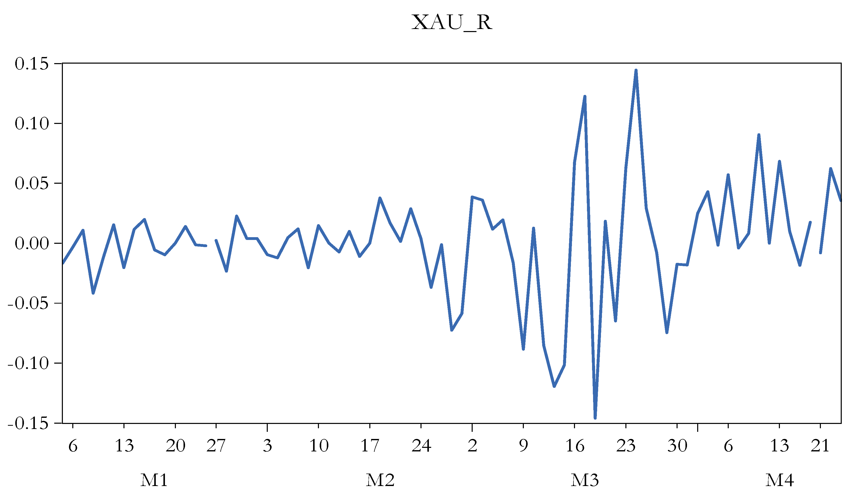
| XAU_R | The daily percentage change of close price of Philadelphia Gold/Silver Index | Thomson Reuters Eikon |
| Variables regarding currencies | ||
| EUR_CNY | The daily percentage change of EUR/CNY | Investing.com |
| Variables regarding 10-Year Government Bond Spreads | ||
| RO_BOND | The daily percentage change of the Romanian 10-year bond yield | Investing.com |
| Variables | Mean | Median | Standard Deviation | Skewness | Kurtosis | Jarque–Bera | Probability |
|---|---|---|---|---|---|---|---|
| NC_CH | 887.5000 | 98.5000 | 2040.816 | 5.02 | 34.31 | 3243.22 | 0.00 |
| ND_CH | 33.0278 | 10.5000 | 47.9956 | 2.13 | 8.31 | 138.78 | 0.00 |
| NC_IT | 1521.139 | 95.0000 | 1934.999 | 0.78 | 1.99 | 10.45 | 0.01 |
| ND_IT | 208.0139 | 4.5000 | 279.6809 | 0.85 | 2.06 | 11.23 | 0.00 |
| DJIA_R | −0.002321 | 0.0000 | 0.0371 | −0.39 | 5.89 | 2.88 | 0.00 |
| SPX_R | −0.0024 | 0.0001 | 0.0341 | −0.67 | 5.76 | 28.26 | 0.00 |
| IBEX35_R | −0.0052 | −0.0008 | 0.0301 | −1.69 | 10.65 | 210.03 | 0.00 |
| FTMIB_R | −0.0052 | 0.0013 | 0.0337 | −2.53 | 14.67 | 485.29 | 0.00 |
| FCHI_R | −0.0038 | 0.0003 | 0.0299 | −1.16 | 7.51 | 77.15 | 0.00 |
| GDAXI_R | −0.0029 | 0.0001 | 0.0299 | −0.83 | 8.67 | 104.56 | 0.00 |
| FTSE_R | −0.0035 | 0.0000 | 0.0260 | −0.93 | 8.62 | 105.12 | 0.00 |
| SSE100_R | 0.0000 | 0.0003 | 0.0190 | −1.65 | 8.49 | 123.27 | 0.00 |
| BET_R | −0.0031 | −0.0007 | 0.0250 | −0.96 | 6.58 | 49.60 | 0.00 |
| CRUDE_OIL | 40.9738 | 49.1500 | 17.6997 | −1.35 | 6.37 | 56.07 | 0.00 |
| WTI | 40.9296 | 49.1300 | 17.8440 | −1.33 | 6.05 | 49.03 | 0.00 |
| NATURAL_GAS | 1.8352 | 1.8270 | 0.1604 | 0.57 | 2.88 | 4.01 | 0.13 |
| LSCO | 41.0201 | 48.1050 | 15.5022 | −0.43 | 1.69 | 7.41 | 0.02 |
| XAU_R | 0.0041 | 0.0040 | 0.0455 | −0.25 | 5.61 | 21.14 | 0.00 |
| EUR_CNY | −0.0002 | 0.0000 | 0.0058 | 0.06 | 4.17 | 4.13 | 0.13 |
| RO_BOND | 0.0013 | 0.0000 | 0.0535 | −1.52 | 15.66 | 508.19 | 0.00 |
| Variables | NC_CH | ND_CH | NC_IT | ND_IT | DJIA_R | SPX_R | IBEX35_R | FTMIB_R | FCHI_R | GDAXI_R |
| NC_CH | 1.0000 | |||||||||
| ND_CH | 0.7347 | 1.0000 | ||||||||
| NC_IT | −0.3117 | −0.4345 | 1.0000 | |||||||
| ND_IT | −0.2954 | −0.4332 | 0.9425 | 1.0000 | ||||||
| DJIA_R | 0.0232 | −0.0618 | 0.0900 | 0.0822 | 1.0000 | |||||
| SPX_R | 0.0311 | −0.0606 | 0.0908 | 0.0807 | 0.9942 | 1.0000 | ||||
| IBEX35_R | 0.0906 | −0.0223 | 0.0646 | 0.0726 | 0.7555 | 0.7530 | 1.0000 | |||
| FTMIB_R | 0.0892 | −0.0314 | 0.0702 | 0.0977 | 0.7122 | 0.7113 | 0.8734 | 1.0000 | ||
| FCHI_R | 0.0623 | −0.0466 | 0.1109 | 0.1300 | 0.7406 | 0.7261 | 0.8585 | 0.9100 | 1.0000 | |
| GDAXI_R | 0.0616 | −0.0623 | 0.1343 | 0.1639 | 0.7313 | 0.7165 | 0.8419 | 0.9095 | 0.9740 | 1.0000 |
| FTSE_R | 0.0129 | −0.0687 | 0.1094 | 0.1318 | 0.7864 | 0.7776 | 0.9130 | 0.8539 | 0.8994 | 0.8880 |
| SSE100_R | −0.0054 | 0.0591 | −0.0128 | 0.0203 | 0.3293 | 0.3124 | 0.3615 | 0.3055 | 0.3959 | 0.3793 |
| BET_R | 0.0839 | −0.0117 | 0.0697 | 0.0743 | 0.7429 | 0.7346 | 0.7759 | 0.6505 | 0.7256 | 0.7308 |
| CRUDE_OIL | 0.2257 | 0.3237 | −0.8135 | −0.8392 | −0.0701 | −0.0799 | 0.0210 | −0.0508 | −0.0674 | −0.0863 |
| WTI | 0.2257 | 0.3266 | −0.8278 | −0.8529 | −0.0852 | −0.0954 | 0.0039 | −0.0685 | −0.0903 | −0.1114 |
| NATURAL_GAS | 0.0176 | 0.0215 | −0.6981 | −0.6758 | 0.0533 | 0.0569 | 0.0347 | 0.0382 | 0.0286 | 0.0160 |
| LSCO | 0.2691 | 0.3657 | −0.8894 | −0.8932 | −0.0013 | −0.0085 | 0.0379 | 0.0202 | 0.0023 | −0.0199 |
| XAU_R | 0.0164 | 0.0147 | 0.1509 | 0.1904 | 0.4163 | 0.3999 | 0.4578 | 0.3668 | 0.4591 | 0.5018 |
| EUR_CNY | −0.0433 | 0.0326 | −0.0121 | −0.0208 | −0.3536 | −0.3785 | −0.2787 | −0.3529 | −0.3018 | −0.3107 |
| RO_BOND | −0.0966 | −0.0654 | −0.0054 | −0.0517 | −0.0705 | −0.0268 | −0.1075 | −0.1446 | −0.2031 | −0.1371 |
| Variables | FTSE_R | SSE100_R | BET_R | CRUDE_OIL | WTI | NATURAL_GAS | LSCO | XAU_R | EUR_CNY | RO_BOND |
| FTSE_R | 1.0000 | |||||||||
| SSE100_R | 0.3919 | 1.0000 | ||||||||
| BET_R | 0.7797 | 0.5072 | 1.0000 | |||||||
| CRUDE_OIL | −0.1034 | −0.0060 | −0.0341 | 1.0000 | ||||||
| WTI | −0.1252 | −0.0231 | −0.0552 | 0.9953 | 1.0000 | |||||
| NATURAL_GAS | 0.0726 | 0.0763 | 0.0807 | 0.6400 | 0.6439 | 1.0000 | ||||
| LSCO | −0.0307 | 0.0508 | 0.0520 | 0.9431 | 0.9431 | 0.7375 | 1.0000 | |||
| XAU_R | 0.5626 | 0.2167 | 0.4947 | −0.1737 | −0.1705 | −0.0435 | −0.0922 | 1.0000 | ||
| EUR_CNY | −0.2887 | −0.1657 | −0.2814 | 0.0790 | 0.0692 | −0.1192 | 0.0006 | −0.1494 | 1.0000 | |
| RO_BOND | −0.1471 | −0.1831 | −0.0734 | −0.0311 | −0.0289 | −0.0089 | −0.0442 | −0.0899 | −0.3658 | 1.0000 |
| Variable | Level | 1st Difference | Integration Order |
|---|---|---|---|
| Prob.* | Prob.* | ||
| NC_CH | 0.016 | 0 | I(0) |
| ND_CH | 0.6591 | 0.0001 | I(1) |
| NC_IT | 0.7764 | 0 | I(1) |
| ND_IT | 0.7121 | 0.0265 | I(1) |
| DJIA_R | 0.0867 | 0 | I(1) |
| SPX_R | 0.4132 | 0.0001 | I(1) |
| IBEX35_R | 0.1097 | 0.0001 | I(1) |
| FTMIB_R | 0.0738 | 0.0001 | I(1) |
| FCHI_R | 0.0719 | 0 | I(1) |
| GDAXI_R | 0.3611 | 0.0001 | I(1) |
| FTSE_R | 0.3798 | 0.0001 | I(1) |
| SSE100_R | 0.0301 | 0.0001 | I(0) |
| BET_R | 0.0865 | 0.0001 | I(1) |
| CRUDE_OIL | 0.9977 | 0.0001 | I(1) |
| WTI | 0.9963 | 0.0001 | I(1) |
| NATURAL_GAS | 0.2127 | 0 | I(1) |
| LSCO | 0.9689 | 0 | I(1) |
| XAU_R | 0 | 0 | I(0) |
| EUR_CNY | 0 | 0 | I(0) |
| RO_BOND | 0.0003 | 0 | I(0) |
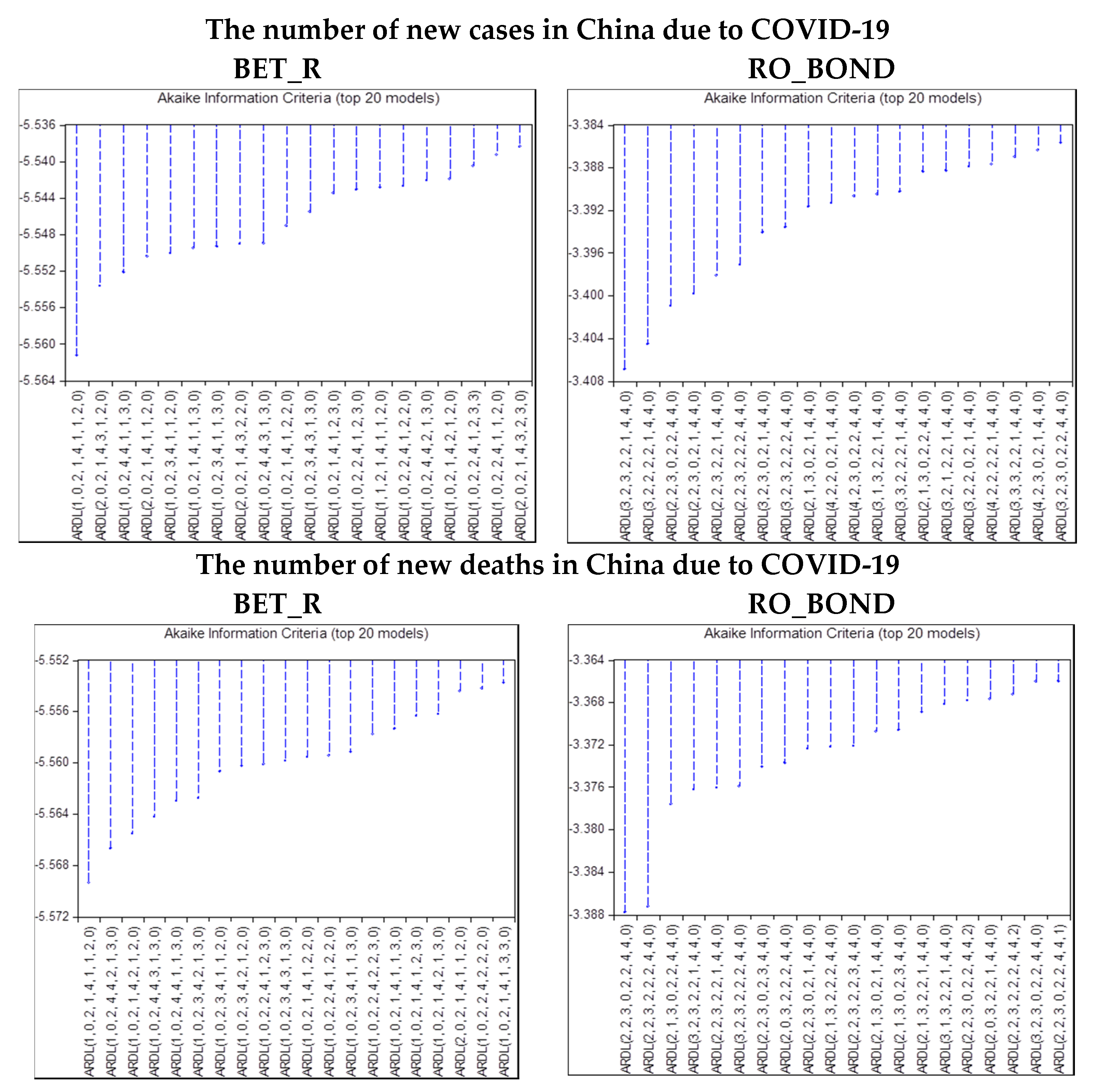
| ARDL—The Number of New Cases in China due to COVID-19 | |
| BET_R | ARDL(1, 0, 2, 1, 4, 1, 1, 2, 0) |
| RO_BOND | ARDL(3, 2, 3, 2, 2, 1, 4, 4, 0) |
| ARDL—The Number of New Deaths in China due to COVID-19 | |
| BET_R | ARDL(1, 0, 2, 1, 4, 1, 1, 2, 0) |
| RO_BOND | ARDL(2, 2, 3, 0, 2, 2, 4, 4, 0) |
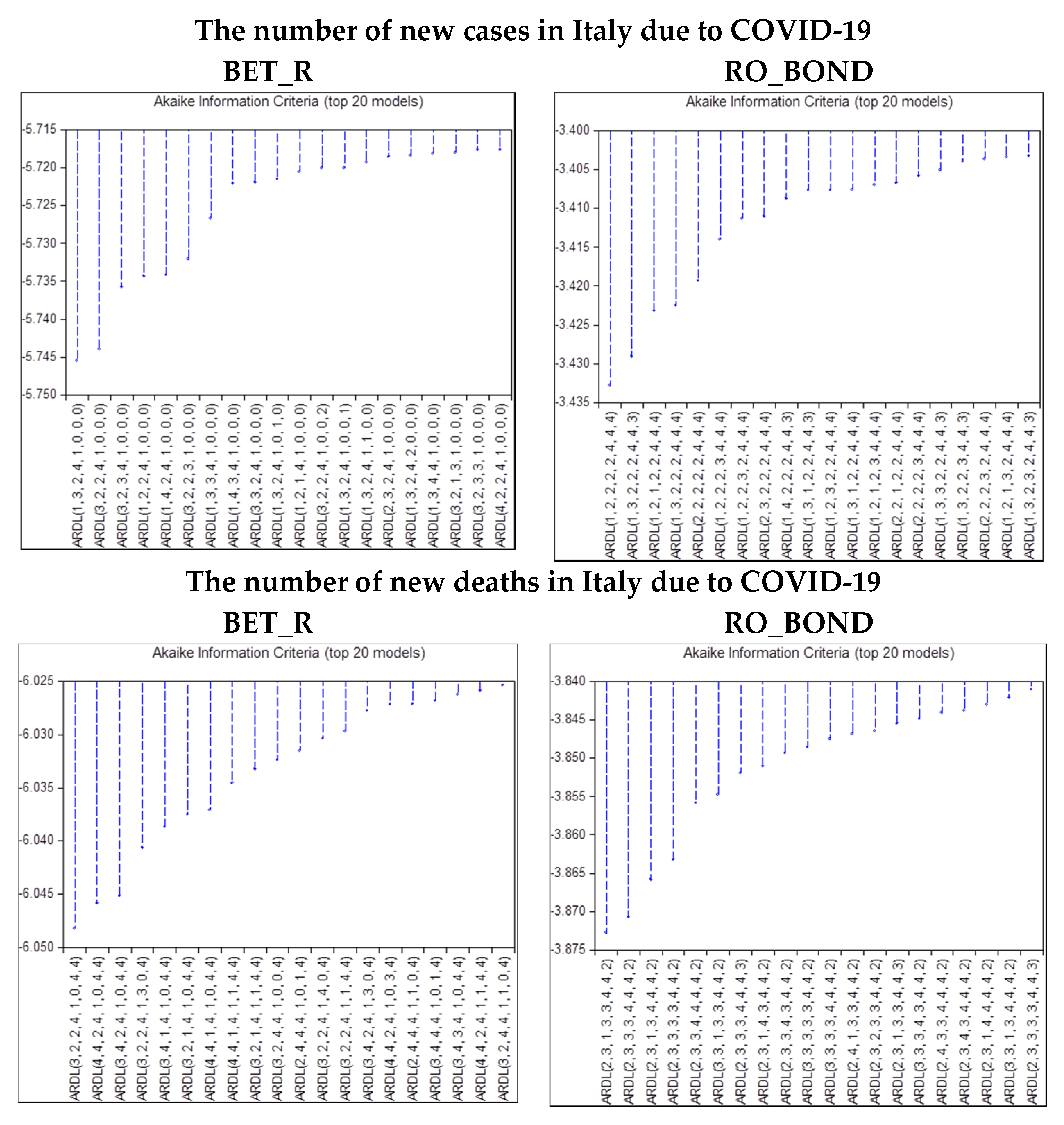
| ARDL—The number of new cases in Italy due to COVID-19 | |
| BET_R | ARDL(1, 3, 2, 4, 1, 0, 0, 0) |
| RO_BOND | ARDL(1, 2, 2, 2, 2, 4, 4, 4) |
| ARDL—The number of new deaths in Italy due to COVID-19 | |
| BET_R | ARDL(3, 2, 2, 4, 1, 0, 4, 4) |
| RO_BOND | ARDL(2, 3, 1, 3, 3, 4, 4, 2) |
| Null Hypothesis: No Long-Run Relationships Exist | F-Statistic | |
| The number of new cases in China due to COVID-19 | ||
| BET_R | 18.06988 | |
| RO_BOND | 4.523219 | |
| The number of new deaths in China due to COVID-19 | ||
| BET_R | 18.40808 | |
| RO_BOND | 5.358775 | |
| Critical Value Bounds | ||
| Significance | I0 Bound | I1 Bound |
| 10% | 1.95 | 3.06 |
| 5% | 2.22 | 3.39 |
| 2.50% | 2.48 | 3.7 |
| 1% | 2.79 | 4.1 |
| Null Hypothesis: No Long-Run Relationships Exist | F-Statistic | |
| The number of new cases in Italy due to COVID-19 | ||
| BET_R | 21.68051 | |
| RO_BOND | 7.294209 | |
| The number of new deaths in Italy due to COVID-19 | ||
| BET_R | 18.94637 | |
| RO_BOND | 5.32708 | |
| Critical Value Bounds | ||
| Significance | I0 Bound | I1 Bound |
| 10% | 2.03 | 3.13 |
| 5% | 2.32 | 3.5 |
| 2.50% | 2.6 | 3.84 |
| 1% | 2.96 | 4.26 |
| ARDL—The Number of New Cases in China due to COVID-19 | |||||
|---|---|---|---|---|---|
| BET_R | |||||
| Variables | Coefficient | Std. Error | t-Statistic | Prob. | CointEq (−1) |
| SSE100_R | 0.1616 | 0.1043 | 1.5489 | 0.1275 | −1.017783(0) |
| EUR_CNY | −1.3775 | 0.6322 | −2.1790 | 0.0339 | |
| LSCO | −0.0016 | 0.0009 | −1.6941 | 0.0962 | |
| XAU_R | 0.2983 | 0.0956 | 3.1188 | 0.0030 | |
| NATURAL_GAS | −0.0022 | 0.0203 | −0.1062 | 0.9159 | |
| CRUDE_OIL | 0.0068 | 0.0020 | 3.3857 | 0.0014 | |
| WTI | −0.0050 | 0.0015 | −3.3472 | 0.0015 | |
| NC_CH | 0.0000 | 0.0000 | 0.5168 | 0.6075 | |
| C | −0.0110 | 0.0292 | −0.3753 | 0.7090 | |
| RO_BOND | |||||
| Variables | Coefficient | Std. Error | t-Statistic | Prob. | CointEq (−1) |
| SSE100_R | −0.73407 | 0.317581 | −2.31143 | 0.0257 | −1.853068 (0) |
| EUR_CNY | −3.33276 | 1.262391 | −2.64004 | 0.0115 | |
| LSCO | 0.000428 | 0.001982 | 0.21588 | 0.8301 | |
| XAU_R | −0.3718 | 0.140512 | −2.64602 | 0.0113 | |
| NATURAL_GAS | −0.0295 | 0.034367 | −0.85833 | 0.3955 | |
| CRUDE_OIL | −0.00673 | 0.00448 | −1.50213 | 0.1404 | |
| WTI | 0.006189 | 0.003557 | 1.74007 | 0.089 | |
| NC_CH | −2E-06 | 0.000001 | −1.22238 | 0.2282 | |
| C | 0.061438 | 0.050715 | 1.21143 | 0.2323 | |
| ARDL—The number of new deaths in China due to COVID-19 | |||||
|---|---|---|---|---|---|
| BET_R | |||||
| Variables | Coefficient | Std. Error | t-Statistic | Prob. | CointEq (−1) |
| SSE100_R | 0.161344 | 0.103218 | 1.563134 | 0.1241 | −1.022253 (0) |
| EUR_CNY | −1.40622 | 0.619485 | −2.26998 | 0.0274 | |
| LSCO | −0.00116 | 0.000982 | −1.18237 | 0.2424 | |
| XAU_R | 0.307503 | 0.094295 | 3.261086 | 0.002 | |
| NATURAL_GAS | −0.01098 | 0.020597 | −0.53307 | 0.5963 | |
| CRUDE_OIL | 0.00646 | 0.002033 | 3.176981 | 0.0025 | |
| WTI | −0.0049 | 0.00148 | −3.31281 | 0.0017 | |
| ND_CH | −3.5E-05 | 0.000041 | −0.8348 | 0.4077 | |
| C | 0.000795 | 0.029663 | 0.026797 | 0.9787 | |
| RO_BOND | |||||
| Variables | Coefficient | Std. Error | t-Statistic | Prob. | CointEq (−1) |
| SSE100_R | −0.8325 | 0.375288 | −2.21829 | 0.0316 | −1.578551 (0) |
| EUR_CNY | −2.29762 | 1.480246 | −1.55219 | 0.1276 | |
| LSCO | −0.00106 | 0.001518 | −0.69786 | 0.4889 | |
| XAU_R | −0.46095 | 0.162187 | −2.84208 | 0.0067 | |
| NATURAL_GAS | 0.007984 | 0.045281 | 0.176315 | 0.8608 | |
| CRUDE_OIL | −0.00652 | 0.005282 | −1.23372 | 0.2237 | |
| WTI | 0.006963 | 0.004186 | 1.663637 | 0.1031 | |
| ND_CH | 0.000009 | 0.000084 | 0.103675 | 0.9179 | |
| C | 0.014044 | 0.066547 | 0.211036 | 0.8338 | |
| Breusch–Godfrey Serial Correlation LM Test | |||
|---|---|---|---|
| ARDL—The number of new cases in China due to COVID-19 | |||
| BET_R | |||
| F-statistic | 1.3637 | Prob. F(2,50) | 0.2651 |
| Obs*R-squared | 3.77603 | Prob. Chi-Square(2) | 0.1514 |
| RO_BOND | |||
| F-statistic | 1.551194 | Prob. F(2,41) | 0.2242 |
| Obs*R-squared | 5.135193 | Prob. Chi-Square(2) | 0.0767 |
| ARDL—The number of new deaths in China due to COVID-19 | |||
| BET_R | |||
| F-statistic | 0.752052 | Prob. F(2,50) | 0.4767 |
| Obs*R-squared | 2.131861 | Prob. Chi-Square(2) | 0.3444 |
| RO_BOND | |||
| F-statistic | 2.743942 | Prob. F(2,43) | 0.0756 |
| Obs*R-squared | 8.262179 | Prob. Chi-Square(2) | 0.0161 |
| Heteroscedasticity Test: Breusch–Pagan–Godfrey | |||
|---|---|---|---|
| ARDL—The number of new cases in China due to COVID-19 | |||
| BET_R | |||
| F-statistic | 1.998167 | Prob. F(20,52) | 0.0237 |
| Obs*R-squared | 31.72268 | Prob. Chi-Square(20) | 0.0463 |
| RO_BOND | |||
| F-statistic | 1.088975 | Prob. F(29,43) | 0.3929 |
| Obs*R-squared | 30.91112 | Prob. Chi-Square(29) | 0.3696 |
| ARDL—The number of new deaths in China due to COVID-19 | |||
| BET_R | |||
| F-statistic | 1.228936 | Prob. F(20,52) | 0.2699 |
| Obs*R-squared | 23.43009 | Prob. Chi-Square(20) | 0.2682 |
| RO_BOND | |||
| F-statistic | 1.062309 | Prob. F(27,45) | 0.4193 |
| Obs*R-squared | 28.41672 | Prob. Chi-Square(27) | 0.3897 |
| ARDL—The Number of New Cases in Italy due to COVID-19 | |||||
|---|---|---|---|---|---|
| BET_R | |||||
| Variables | Coefficient | Std. Error | t-Statistic | Prob. | CointEq (−1) |
| FTMIB_R | 0.2859 | 0.1377 | 2.0760 | 0.0427 | −0.954393 (0) |
| LSCO | −0.0003 | 0.0006 | −0.4545 | 0.6513 | |
| XAU_R | 0.1963 | 0.1074 | 1.8279 | 0.0731 | |
| NATURAL_GAS | 0.0123 | 0.0163 | 0.7532 | 0.4546 | |
| CRUDE_OIL | 0.0024 | 0.0013 | 1.8294 | 0.0729 | |
| WTI | −0.0021 | 0.0012 | −1.7002 | 0.0948 | |
| NC_IT | 0.0000 | 0.0000 | 0.0103 | 0.9918 | |
| C | −0.0256 | 0.0295 | −0.8669 | 0.3898 | |
| RO_BOND | |||||
| Variables | Coefficient | Std. Error | t-Statistic | Prob. | CointEq (−1) |
| FTMIB_R | 0.5133 | 0.3556 | 1.4437 | 0.1559 | −1.147405 (0) |
| LSCO | −0.0068 | 0.0041 | −1.6445 | 0.1072 | |
| XAU_R | −0.7336 | 0.2267 | −3.2362 | 0.0023 | |
| NATURAL_GAS | 0.1743 | 0.0593 | 2.9375 | 0.0052 | |
| CRUDE_OIL | 0.0185 | 0.0087 | 2.1270 | 0.0391 | |
| WTI | −0.0187 | 0.0073 | −2.5465 | 0.0145 | |
| NC_IT | 0.0000 | 0.0000 | −3.0230 | 0.0042 | |
| C | 0.0342 | 0.0866 | 0.3944 | 0.6952 | |
| ARDL—The Number of New Deaths in Italy due to COVID-19 | |||||
|---|---|---|---|---|---|
| BET_R | |||||
| Variables | Coefficient | Std. Error | t-Statistic | Prob. | CointEq (−1) |
| FTMIB_R | 0.3143 | 0.0643 | 4.8907 | 0.0000 | −1.647813 (0) |
| LSCO | −0.0009 | 0.0005 | −1.6594 | 0.1040 | |
| XAU_R | 0.1574 | 0.0662 | 2.3773 | 0.0218 | |
| NATURAL_GAS | −0.0108 | 0.0107 | −1.0016 | 0.3219 | |
| CRUDE_OIL | 0.0027 | 0.0008 | 3.4207 | 0.0013 | |
| WTI | −0.0013 | 0.0007 | −1.8479 | 0.0712 | |
| ND_IT | 0.0000 | 0.0000 | 1.3777 | 0.1751 | |
| C | −0.0045 | 0.0153 | −0.2954 | 0.7691 | |
| RO_BOND | |||||
| Variables | Coefficient | Std. Error | t-Statistic | Prob. | CointEq (−1) |
| FTMIB_R | 0.1323 | 0.3058 | 0.4327 | 0.6674 | −1.204853(0) |
| LSCO | −0.0105 | 0.0029 | −3.6061 | 0.0008 | |
| XAU_R | −0.5498 | 0.2305 | −2.3852 | 0.0216 | |
| NATURAL_GAS | 0.1286 | 0.0571 | 2.2515 | 0.0295 | |
| CRUDE_OIL | 0.0240 | 0.0085 | 2.8202 | 0.0072 | |
| WTI | −0.0192 | 0.0076 | −2.5115 | 0.0159 | |
| ND_IT | −0.0002 | 0.0001 | −2.7338 | 0.0091 | |
| C | 0.0504 | 0.0632 | 0.7967 | 0.4300 | |
| Breusch–Godfrey Serial Correlation LM Test: | |||
|---|---|---|---|
| ARDL—The number of new cases in Italy due to COVID-19 | |||
| BET_R | |||
| F-statistic | 0.636347 | Prob. F(2,52) | 0.5333 |
| Obs*R-squared | 1.743982 | Prob. Chi-Square(2) | 0.4181 |
| RO_BOND | |||
| F-statistic | 1.679769 | Prob. F(4,40) | 0.1737 |
| Obs*R-squared | 10.49876 | Prob. Chi-Square(4) | 0.0328 |
| ARDL—The number of new deaths in Italy due to COVID-19 | |||
| BET_R | |||
| F-statistic | 0.057834 | Prob. F(2,43) | 0.9439 |
| Obs*R-squared | 0.19584 | Prob. Chi-Square(2) | 0.9067 |
| RO_BOND | |||
| F-statistic | 2.062798 | Prob. F(2,41) | 0.1401 |
| Obs*R-squared | 6.674006 | Prob. Chi-Square(2) | 0.0355 |
| Heteroscedasticity Test: Breusch–Pagan–Godfrey | |||
|---|---|---|---|
| ARDL—The number of new cases in Italy due to COVID-19 | |||
| BET_R | |||
| F-statistic | 1.708739 | Prob. F(18,54) | 0.0665 |
| Obs*R-squared | 26.49074 | Prob. Chi-Square(18) | 0.0891 |
| RO_BOND | |||
| F-statistic | 0.693446 | Prob. F(28,44) | 0.8464 |
| Obs*R-squared | 22.35071 | Prob. Chi-Square(28) | 0.7648 |
| ARDL—The number of new deaths in Italy due to COVID-19 | |||
| BET_R | |||
| F-statistic | 0.80796 | Prob. F(27,45) | 0.7191 |
| Obs*R-squared | 23.83434 | Prob. Chi-Square(27) | 0.6395 |
| RO_BOND | |||
| F-statistic | 0.626455 | Prob. F(29,43) | 0.9063 |
| Obs*R-squared | 21.68164 | Prob. Chi-Square(29) | 0.8331 |
| Null Hypothesis | 1st Lag | 2nd Lag | 3rd Lag | |||
|---|---|---|---|---|---|---|
| F-Statistic | Prob. | F-Statistic | Prob. | F-Statistic | Prob. | |
| DFCHI_R does not Granger Cause DBET_R | 2.6267 | 0.1095 | 1.37666 | 0.2593 | 1.03323 | 0.3837 |
| DBET_R does not Granger Cause DFCHI_R | 0.01526 | 0.902 | 0.67225 | 0.5139 | 2.73881 | 0.0503 |
| DWTI does not Granger Cause DBET_R | 0.32344 | 0.5713 | 0.15567 | 0.8561 | 0.89465 | 0.4487 |
| DBET_R does not Granger Cause DWTI | 0.66746 | 0.4166 | 0.55401 | 0.5772 | 0.60479 | 0.6142 |
| DCRUDE_OIL does not Granger Cause DBET_R | 1.64744 | 0.2034 | 1.19169 | 0.3099 | 1.54876 | 0.2102 |
| DBET_R does not Granger Cause DCRUDE_OIL | 1.40219 | 0.2403 | 0.74496 | 0.4785 | 1.09251 | 0.3585 |
| DGDAXI_R does not Granger Cause DBET_R | 0.54561 | 0.4625 | 1.70531 | 0.1893 | 1.15653 | 0.333 |
| DBET_R does not Granger Cause DGDAXI_R | 0.63702 | 0.4274 | 1.82947 | 0.1682 | 2.55856 | 0.0625 |
| DDJIA_R does not Granger Cause DBET_R | 0.08379 | 0.7731 | 1.01848 | 0.3665 | 1.24507 | 0.3005 |
| DBET_R does not Granger Cause DDJIA_R | 1.91735 | 0.1704 | 0.54163 | 0.5843 | 0.36964 | 0.7752 |
| DFTSE_R does not Granger Cause DBET_R | 0.14757 | 0.702 | 1.46304 | 0.2386 | 0.94017 | 0.4264 |
| DBET_R does not Granger Cause DFTSE_R | 0.34236 | 0.5603 | 0.82895 | 0.4408 | 0.90187 | 0.4451 |
| DFTMIB_R does not Granger Cause DBET_R | 3.9811 | 0.0498 | 0.68299 | 0.5085 | 2.40174 | 0.0755 |
| DBET_R does not Granger Cause DFTMIB_R | 2.40769 | 0.1251 | 1.63062 | 0.2033 | 1.53362 | 0.214 |
| DIBEX35_R does not Granger Cause DBET_R | 5.99134 | 0.0168 | 5.79833 | 0.0047 | 3.77034 | 0.0146 |
| DBET_R does not Granger Cause DIBEX35_R | 5.93584 | 0.0173 | 2.58061 | 0.083 | 3.46318 | 0.0211 |
| DJIA_R does not Granger Cause DBET_R | 4.84108 | 0.031 | 2.32679 | 0.1052 | 3.07207 | 0.0337 |
| DBET_R does not Granger Cause DJIA_R | 3.6263 | 0.0609 | 0.96526 | 0.386 | 0.85631 | 0.4683 |
| DNATURAL_G does not Granger Cause DBET_R | 2.61024 | 0.1105 | 3.06162 | 0.0532 | 2.01611 | 0.1202 |
| DBET_R does not Granger Cause DNATURAL_G | 4.6538 | 0.0343 | 2.93068 | 0.06 | 2.76934 | 0.0485 |
| DNC_IT does not Granger Cause DBET_R | 1.88151 | 0.1744 | 0.24766 | 0.7813 | 2.31234 | 0.0841 |
| DBET_R does not Granger Cause DNC_IT | 6.78189 | 0.0112 | 3.57262 | 0.0334 | 3.72495 | 0.0155 |
| DND_CH does not Granger Cause DBET_R | 0.00174 | 0.9668 | 0.00364 | 0.9964 | 0.00707 | 0.9992 |
| DBET_R does not Granger Cause DND_CH | 0.00076 | 0.9781 | 0.00208 | 0.9979 | 0.02642 | 0.9941 |
| DND_IT does not Granger Cause DBET_R | 1.14888 | 0.2874 | 0.76009 | 0.4715 | 0.49269 | 0.6886 |
| DBET_R does not Granger Cause DND_IT | 0.00748 | 0.9313 | 0.67359 | 0.5132 | 1.80249 | 0.1553 |
| DLSCO does not Granger Cause DBET_R | 0.03988 | 0.8423 | 0.9342 | 0.3978 | 0.91111 | 0.4405 |
| DBET_R does not Granger Cause DLSCO | 7.33898 | 0.0084 | 5.77264 | 0.0048 | 3.88014 | 0.0129 |
| DSPX_R does not Granger Cause DBET_R | 0.17873 | 0.6737 | 1.34967 | 0.2661 | 1.65264 | 0.1858 |
| DBET_R does not Granger Cause DSPX_R | 1.82924 | 0.1804 | 0.52552 | 0.5936 | 0.34511 | 0.7928 |
| SSE100_R does not Granger Cause DBET_R | 7.74827 | 0.0069 | 4.02162 | 0.0223 | 2.87382 | 0.0428 |
| DBET_R does not Granger Cause SSE100_R | 0.34946 | 0.5563 | 0.65952 | 0.5203 | 2.16779 | 0.1001 |
| EUR_CNY does not Granger Cause DBET_R | 0.21832 | 0.6417 | 0.61712 | 0.5424 | 0.66098 | 0.579 |
| DBET_R does not Granger Cause EUR_CNY | 11.4005 | 0.0012 | 4.48184 | 0.0148 | 2.86132 | 0.0434 |
| NC_CH does not Granger Cause DBET_R | 0.02747 | 0.8688 | 0.01495 | 0.9852 | 0.00963 | 0.9987 |
| DBET_R does not Granger Cause NC_CH | 0.01858 | 0.892 | 0.00141 | 0.9986 | 0.02117 | 0.9958 |
| XAU_R does not Granger Cause DBET_R | 8.85791 | 0.004 | 13.0642 | 0.00002 | 8.66267 | 0.00006 |
| DBET_R does not Granger Cause XAU_R | 17.5622 | 0.00008 | 12.3505 | 0.00003 | 9.59776 | 0.00002 |
| Null Hypothesis | 1st Lag | 2nd Lag | 3rd Lag | |||
|---|---|---|---|---|---|---|
| F-Statistic | Prob. | F-Statistic | Prob. | F-Statistic | Prob. | |
| DFCHI_R does not Granger Cause RO_BOND | 7.93244 | 0.0063 | 4.10612 | 0.0207 | 2.96656 | 0.0382 |
| RO_BOND does not Granger Cause DFCHI_R | 5.35818 | 0.0235 | 5.90784 | 0.0043 | 5.71237 | 0.0015 |
| DWTI does not Granger Cause RO_BOND | 1.40788 | 0.2393 | 2.84061 | 0.0652 | 2.52773 | 0.0649 |
| RO_BOND does not Granger Cause DWTI | 1.84894 | 0.1781 | 2.82801 | 0.066 | 1.84005 | 0.1485 |
| DCRUDE_OIL does not Granger Cause RO_BOND | 0.28071 | 0.5979 | 0.18731 | 0.8296 | 1.73016 | 0.1693 |
| RO_BOND does not Granger Cause DCRUDE_OIL | 2.24912 | 0.1381 | 1.54906 | 0.2197 | 0.96236 | 0.4158 |
| DGDAXI_R does not Granger Cause RO_BOND | 8.83453 | 0.004 | 4.36102 | 0.0165 | 3.97272 | 0.0115 |
| RO_BOND does not Granger Cause DGDAXI_R | 6.57828 | 0.0124 | 5.37455 | 0.0068 | 4.73576 | 0.0047 |
| DDJIA_R does not Granger Cause RO_BOND | 8.42463 | 0.0049 | 6.77884 | 0.0021 | 5.22182 | 0.0027 |
| RO_BOND does not Granger Cause DDJIA_R | 2.77374 | 0.1002 | 1.50012 | 0.2303 | 1.15489 | 0.3337 |
| DFTSE_R does not Granger Cause RO_BOND | 7.81722 | 0.0066 | 3.88167 | 0.0253 | 3.42563 | 0.0221 |
| RO_BOND does not Granger Cause DFTSE_R | 2.39641 | 0.126 | 3.53877 | 0.0344 | 3.00637 | 0.0365 |
| DFTMIB_R does not Granger Cause RO_BOND | 24.5669 | 0.000005 | 12.2384 | 0.00003 | 11.8882 | 0.000002 |
| RO_BOND does not Granger Cause DFTMIB_R | 0.03944 | 0.8431 | 0.45054 | 0.6391 | 0.92968 | 0.4313 |
| DIBEX35_R does not Granger Cause RO_BOND | 4.56719 | 0.036 | 2.23299 | 0.1149 | 1.50269 | 0.222 |
| RO_BOND does not Granger Cause DIBEX35_R | 5.16866 | 0.026 | 3.34464 | 0.0411 | 3.60425 | 0.0178 |
| DJIA_R does not Granger Cause RO_BOND | 19.8188 | 0.00003 | 11.5107 | 0.00005 | 7.49281 | 0.0002 |
| RO_BOND does not Granger Cause DJIA_R | 3.31803 | 0.0726 | 0.89821 | 0.4119 | 0.18455 | 0.9065 |
| DNATURAL_GAS does not Granger Cause RO_BOND | 1.33944 | 0.251 | 0.66142 | 0.5194 | 0.45155 | 0.7171 |
| RO_BOND does not Granger Cause DNATURAL_GAS | 0.50062 | 0.4815 | 0.43031 | 0.652 | 1.03227 | 0.3841 |
| DNC_IT does not Granger Cause RO_BOND | 7.62726 | 0.0073 | 4.77217 | 0.0115 | 3.05509 | 0.0344 |
| RO_BOND does not Granger Cause DNC_IT | 0.09051 | 0.7644 | 0.15265 | 0.8587 | 2.58859 | 0.0603 |
| DND_CH does not Granger Cause RO_BOND | 0.01047 | 0.9188 | 0.34077 | 0.7124 | 0.22026 | 0.882 |
| RO_BOND does not Granger Cause DND_CH | 0.10515 | 0.7467 | 0.02699 | 0.9734 | 0.05421 | 0.9832 |
| DND_IT does not Granger Cause RO_BOND | 0.16266 | 0.6879 | 2.83622 | 0.0655 | 3.69605 | 0.016 |
| RO_BOND does not Granger Cause DND_IT | 1.30755 | 0.2566 | 2.40189 | 0.0981 | 2.24727 | 0.091 |
| DLSCO does not Granger Cause RO_BOND | 2.62586 | 0.1095 | 1.35676 | 0.2643 | 0.87127 | 0.4605 |
| RO_BOND does not Granger Cause DLSCO | 0.04223 | 0.8378 | 0.07082 | 0.9317 | 0.28769 | 0.8341 |
| DSPX_R does not Granger Cause RO_BOND | 7.23441 | 0.0089 | 5.2898 | 0.0073 | 3.98772 | 0.0113 |
| RO_BOND does not Granger Cause DSPX_R | 1.93361 | 0.1686 | 0.73046 | 0.4854 | 0.53808 | 0.6578 |
| SSE100_R does not Granger Cause RO_BOND | 5.93434 | 0.0173 | 3.43564 | 0.0377 | 2.88714 | 0.042 |
| RO_BOND does not Granger Cause SSE100_R | 0.16848 | 0.6827 | 0.55591 | 0.5761 | 0.58164 | 0.6291 |
| NC_CH does not Granger Cause RO_BOND | 0.04289 | 0.8365 | 0.01927 | 0.9809 | 0.30151 | 0.8242 |
| RO_BOND does not Granger Cause NC_CH | 0.01696 | 0.8967 | 0.0044 | 0.9956 | 0.00846 | 0.9989 |
© 2020 by the authors. Licensee MDPI, Basel, Switzerland. This article is an open access article distributed under the terms and conditions of the Creative Commons Attribution (CC BY) license (http://creativecommons.org/licenses/by/4.0/).
Share and Cite
Gherghina, Ș.C.; Armeanu, D.Ș.; Joldeș, C.C. Stock Market Reactions to COVID-19 Pandemic Outbreak: Quantitative Evidence from ARDL Bounds Tests and Granger Causality Analysis. Int. J. Environ. Res. Public Health 2020, 17, 6729. https://doi.org/10.3390/ijerph17186729
Gherghina ȘC, Armeanu DȘ, Joldeș CC. Stock Market Reactions to COVID-19 Pandemic Outbreak: Quantitative Evidence from ARDL Bounds Tests and Granger Causality Analysis. International Journal of Environmental Research and Public Health. 2020; 17(18):6729. https://doi.org/10.3390/ijerph17186729
Chicago/Turabian StyleGherghina, Ștefan Cristian, Daniel Ștefan Armeanu, and Camelia Cătălina Joldeș. 2020. "Stock Market Reactions to COVID-19 Pandemic Outbreak: Quantitative Evidence from ARDL Bounds Tests and Granger Causality Analysis" International Journal of Environmental Research and Public Health 17, no. 18: 6729. https://doi.org/10.3390/ijerph17186729
APA StyleGherghina, Ș. C., Armeanu, D. Ș., & Joldeș, C. C. (2020). Stock Market Reactions to COVID-19 Pandemic Outbreak: Quantitative Evidence from ARDL Bounds Tests and Granger Causality Analysis. International Journal of Environmental Research and Public Health, 17(18), 6729. https://doi.org/10.3390/ijerph17186729