NNetEn_2D: Two-Dimensional Neural Network Entropy in Remote Sensing Imagery and Geophysical Mapping

Abstract

Measuring the predictability and complexity of 2D data (image) series using entropy is an essential tool for evaluation of systems’ irregularity and complexity in remote sensing and geophysical mapping. However, the existing methods have some drawbacks related to their strong dependence on method parameters and image rotation. To overcome these difficulties, this study proposes a new method for estimating two-dimensional neural network entropy (NNetEn_2D) for evaluating the regularity or predictability of images using the LogNNet neural network model. The method is based on an algorithm for converting a 2D kernel into a 1D data series followed by NNetEn_2D calculation. An artificial test image was created for the study. We demonstrate the advantage of using circular instead of square kernels through comparison of the invariance of the NNetEn_2D distribution after image rotation. Highest robustness was observed for circular kernels with a radius of R = 5 and R = 6 pixels, with a NNetEn_2D calculation error of no more than 10%, comparable to the distortion of the initial 2D data. The NNetEn_2D entropy calculation method has two main geometric parameters (kernel radius and its displacement step), as well as two neural network hyperparameters (number of training epochs and one of six reservoir filling techniques). We evaluated our method on both remote sensing and geophysical mapping images. Remote sensing imagery (Sentinel-2) shows that brightness of the image does not affect results, which helps keep a rather consistent appearance of entropy maps over time without saturation effects being observed. Surfaces with little texture, such as water bodies, have low NNetEn_2D values, while urban areas have consistently high values. Application to geophysical mapping of rocks to the northwest of southwest Australia is characterized by low to medium entropy and highlights aspects of the geology. These results indicate the success of NNetEn_2D in providing meaningful entropy information for 2D in remote sensing and geophysical applications.

1. Introduction

Advanced interpretation of remote sensing (RS) imagery [1] and geophysical mapping [2] often requires significant processing efforts. Tasks such as classification, segmentation or change detection can be facilitated by deriving advanced features from the original imagery. For instance, to extract high-level features from reflectance data, common approaches include simple ratios, index calculations, texture metrics and manually or automatically constructed filters. The fact that state-of-the-art Deep Learning techniques are often employed in an end-to-end fashion, using the original imagery directly as an input, is often taken as an indication that “hand-crafted” processing pipelines are not necessary anymore [1]. In fact, the feature maps learned by modern convolutional neural networks (CNNs) are highly effective for large-scale image recognition [3], object detection [4] and semantic segmentation [5,6] tasks. Nevertheless, today’s neural networks require extensive resources for training, and the large amounts of labeled data needed [1,7,8] are often not available for typical remote sensing applications. Therefore, using pre-processed feature inputs in combination with reflectance data may help alleviate these limitations, speed up model training and enable higher accuracies.

One useful type of feature input is entropy. Entropy is a measure of uncertainty in data and is adopted for maximization of mutual information in remote sensing data processing. In information theory, the concept of entropy is used to quantify the amount of information necessary to describe the macro state of a system. Different versions of entropies have been applied for the effective automation of various remote sensing analyses. Shannon’s entropy is the most widely used technique for measuring urban sprawl levels [9,10], and exponential entropy is used for image segmentation [11]. Furthermore, entropy is used to avoid overexposure or underexposure of the image and for image quality evaluation [12,13] as well as change detection [14]. Similarly, the processing of geophysical images (magnetic, gravity and hyperspectral) commonly involves “texture mapping” [15,16,17]. Some methods include derivation of the entropy field [18,19,20], but little use is made of such results as a true measure of complexity. It has been shown that magnetic images in particular are multifractal [21], reflecting the organization of magnetic susceptibility within the rock mass. The establishment of entropy fields for such images is another step towards understanding such organization as a dynamic process reflecting deformation, metamorphism and hydrothermal alteration.

There are several 2D calculation models in existence that use approximating probability distributions. Two-dimensional dispersion entropy (DispEn_2D) [22], sample entropy (SampEn_2D) [23], permutation entropy (PerEn_2D) [24] and approximate entropy (ApEn_2D) [25] have been recently proposed as powerful tools for feature extraction from images, such as noise, nonlinearity and randomness, and can be considered as an irregularity measure of images. DispEn_2D and SampEn_2D have the advantage of being insensitive to translation and rotation [22]. Interpretation of the local neighborhood entropy of pixels in an image is one of the most valuable types of pre-processed features for many RS tasks. Typically, such metrics are obtained through the so-called first- and second-order texture metrics, based on quantized images and Gray-Level Co-occurrence Matrices (GLCM), as first proposed in [26]. The pixel-wise entropy metric calculated based on GLCM, however, is not always of high quality, since it is limited to very small kernels that produce a very sparse GLCM. To better capture the heterogeneity throughout an image, one could expand the concept to large kernels, multi-band or multi-temporal imagery; however, this is hampered by excessive processing time.

In this paper, we apply a recently introduced method called NNetEn to remote sensing imagery (Sentinel-2) and geophysical mapping to explore its potential as an image feature for classification or segmentation tasks. The scientific novelty of the presented method is a new approach to estimating the entropy of 2D data using neural networks, with robustness to image rotation. The method was originally applied to large time series datasets, but is used here in a new adaptation to single-band imagery. It computes entropy without approximating probability distributions, but uses the properties of reservoir neural networks, whose classification ability depends on the degree of irregularity of input information transformations in the reservoir.

The rest of the paper is organized as follows. Section 2 describes the structure of LogNNet for NNetEn_1D and the method for two-dimensional NNetEn_2D calculation with circular and square kernels, as well as the structure of test images and the image rotation method. The numerical examples and results are presented in Section 3. Results are discussed in Section 4, followed by conclusions and outlook.

2. Methods

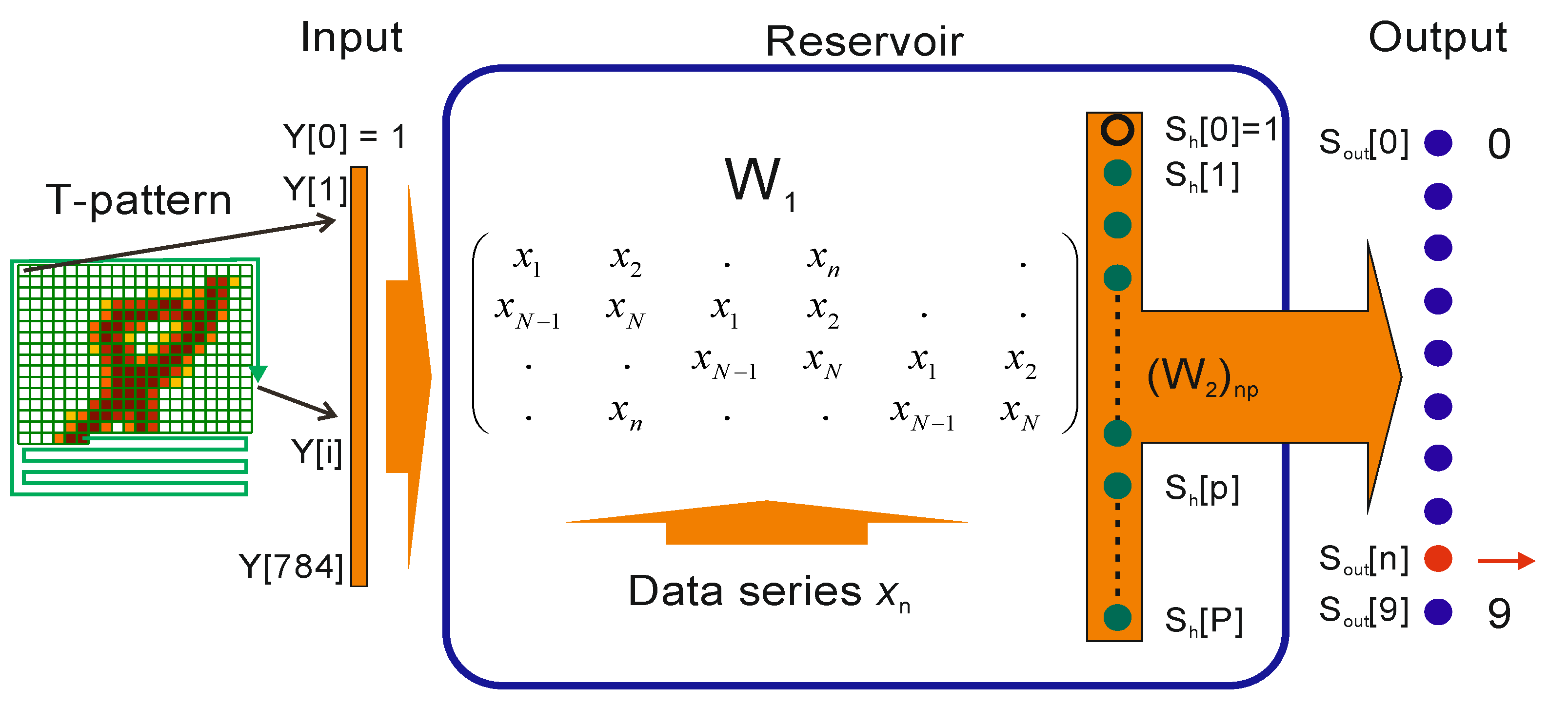
2.1. LogNNet Model for NNetEn_1D Calculation

The LogNNet model [27] was originally designed for recognizing handwritten digits (28 × 28 = 784 pixels) in the MNIST dataset [28]. It comprises three parts (see Figure 1): (a) input layer with vector Y, containing 785 elements corresponding to the brightness of the pixels and the zero element Y [0] = 1, (b) a model reservoir of matrix W₁ to transform the input vector Y into an intermediate vector S_h (maximum element index, p = 25), and (c) a single layer feedforward neural network transforming vector S_h into digits 0–9 in the output layer S_out. Here, we employ a LogNNet model of architecture 784:25:10 [29] to calculate entropy values.

To determine entropy, the LogNNet reservoir matrix is filled with elements of the studied data x_n. The network is then trained and tested on MNIST-10 datasets (60,000 and 10,000 images) to obtain classification accuracy. This accuracy is considered as the entropy measure and denoted as NNetEn_1D.

$${\mathrm{NNetEn}}_{1\mathrm{D}}=\frac{\mathrm{Classification}\mathrm{accuracy}}{100\%}$$

(1)

The procedure for calculating NNetEn_1D is described in more detail in [29].

The maximum number of elements that can be fed to the model is determined by the number of elements in matrix W₁ (N₀ = 19,625). Variations of the techniques for filling the matrix W₁ with a series of data is presented in [30]; they are divided into six methods:

W1M_1: Filling by rows, as in Figure 1, with copying of the series.

W1M_2: Matrix W₁ is reset and filled in by rows, as in Figure 1, “restarting” with the original series at each row.

W1M_3: The original series is converted to a series with N = 19,625 elements using a linear approximation (data series stretch operation). Then, the matrix is filled row by row with a stretched series.

W1M_4: Filling as in the W1M_1 method, but by columns.

W1M_5: Filling as in the W1M_2 method, but by columns.

W1M_6: Filling as in the W1M_3 method, but by columns (series stretching operation by 19,625 elements).

The main method used in this work was the W1M_1 method, except for Section 3.2, where the W1M_1–W1M_6 methods were used.

Method W1M_1 ensured greater stability when working with smaller numbers of input data points (e.g., when using only small local kernels, see Section 2.2). The maximum number of translations NT of a data series x_n of length N can be estimated by the formula

$$NT=⌈\frac{19625}{N}⌉$$

(2)

where ⌈ ⌉ is a ceiling function for rounding up to the nearest higher integer.

The W1M_5 method works well when N > 11,000 [30]. Methods W1M_3 and W1M_6 have increased accuracy if the data represent the dynamics of a certain physical process or obey linear or non-linear equations (for example, the distribution of magnetic fields or other physical quantities). In general, all six methods provide similar results in estimating entropy, but it is the experimenter’s responsibility to determine the best method for a given problem.

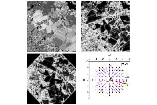
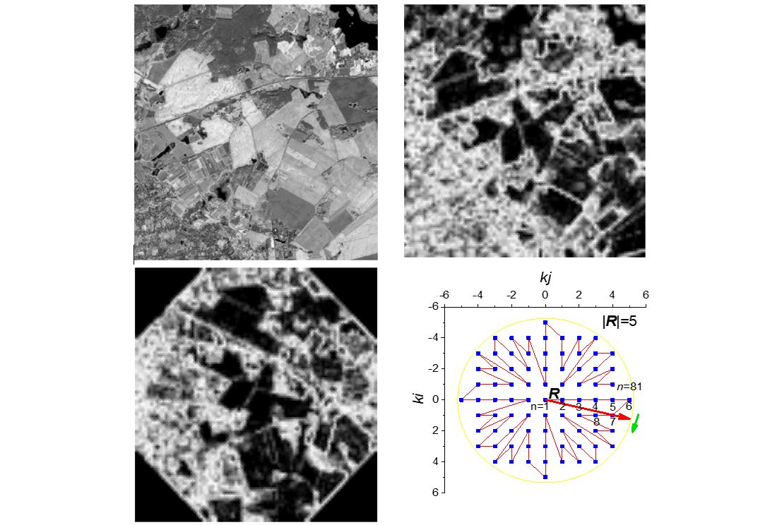
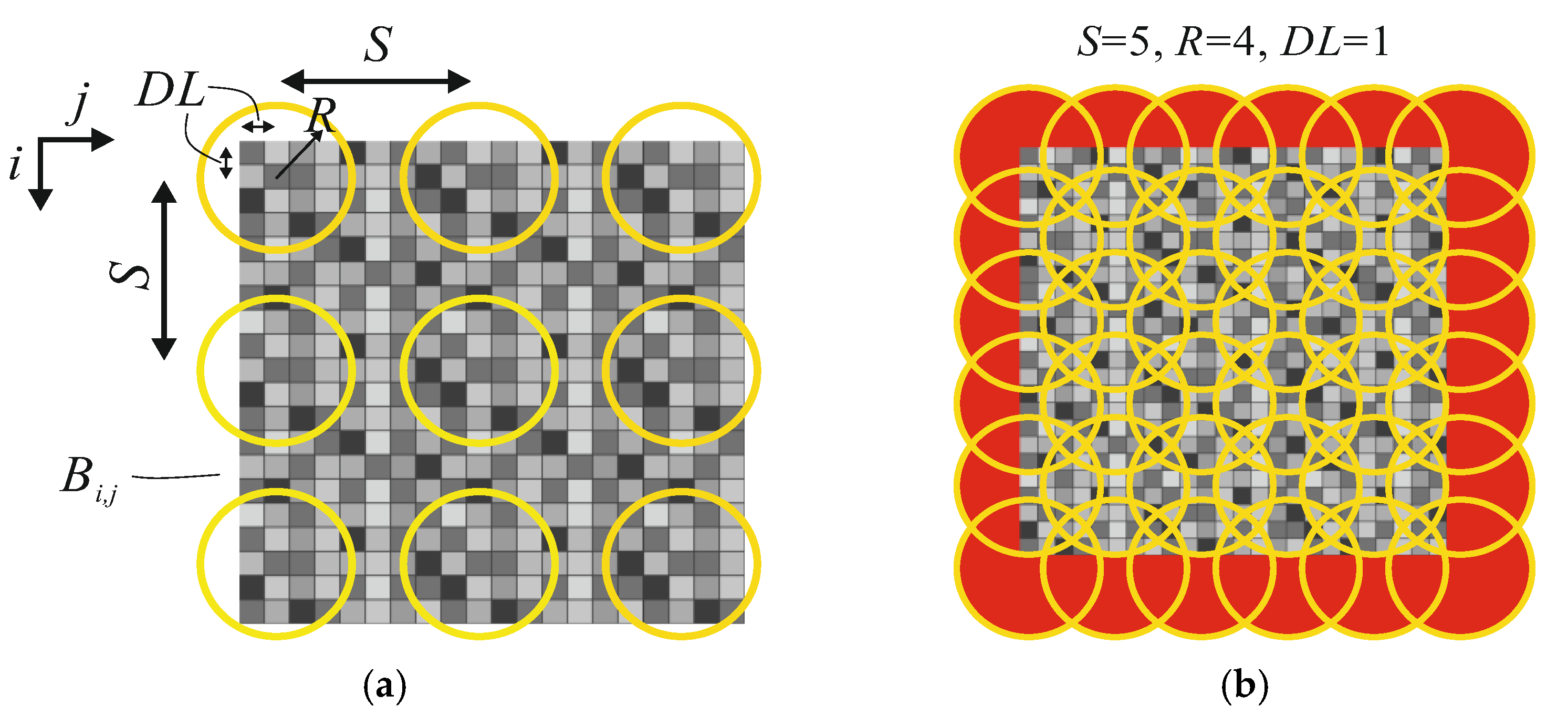
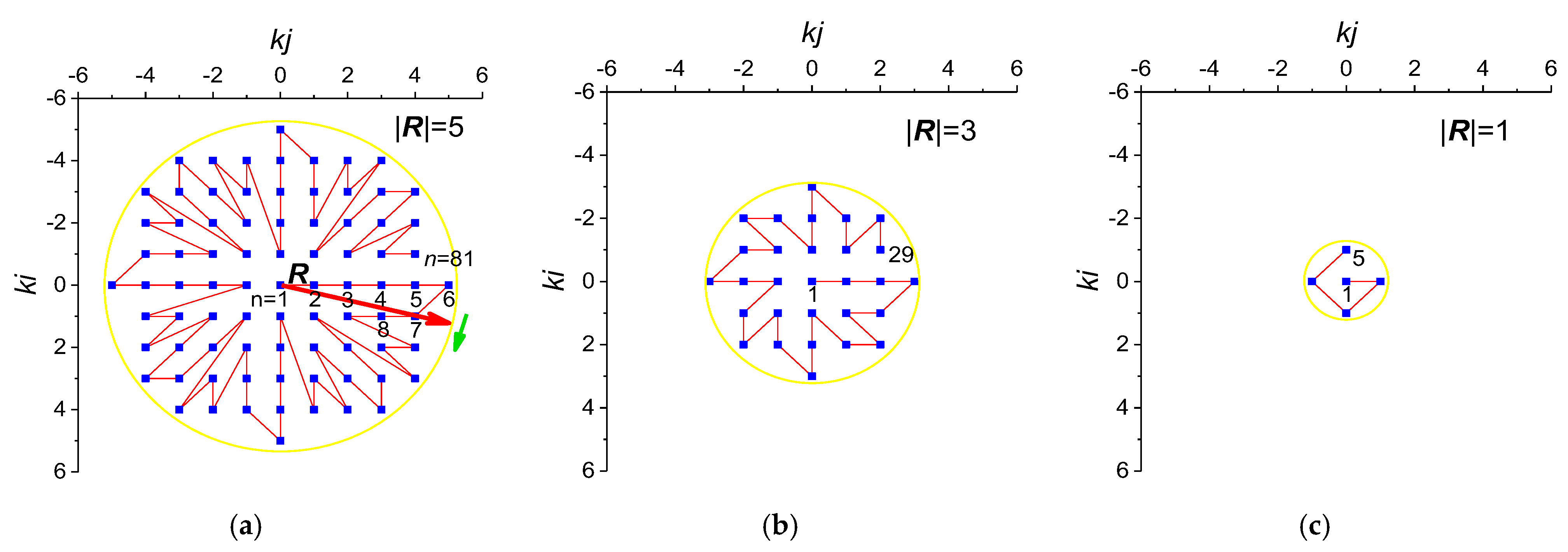
2.2. Method for Two-Dimensional NNetEn_2D Calculation with Circular Kernels

Suppose we have a rectangular grayscale image in which the brightness is represented by an array of pixels B_i,j. To calculate the NNetEn_2D in two-dimensional space, the entire image is divided into local, overlapping windows (kernels) of radius R, moved along both axes with step size S, starting from the upper left corner with the coordinates of the center of the first kernel (DL, DL) (see Figure 2a). The minimum kernel radius R_min for uniform coverage of the entire space can be estimated from the Formula (3)

$$R_{\min }=⌈\frac{\sqrt{2\cdot S^2}}{2}⌉$$

(3)

where S is the step and ⌈ ⌉ is a ceiling function.

R_min series evaluation is shown in

Table 1. Minimum kernel radius R_min versus step size S.

S	1	2	3	4	5	6	7	8	9
Rmin	1	2	3	3	4	5	5	6	7

.

Let us introduce the abbreviated name of the circular kernel CIR_R, where R is the radius, for example, CIR_3, CIR_5.

With S = 5 Formula (3) results in R_min = 4 (CIR_4), the location of the circular kernels in this case is shown in (Figure 2b). Areas that are outside the image boundaries are marked in red, B_i,j values are not defined in these areas, so the pixel values in these areas are filled by symmetrical mirroring of the pixels in the image. If S > 1, the red areas may not be symmetrical on different sides of the pattern; in some cases, symmetry can be restored by selecting the DL value.

The number of pixels N in a circular kernel has a quadratic dependence on the radius N ~ R²; evaluation of sample values is given in

Table 2. Number of pixels N in a circular kernel versus radius R.

R	1	2	3	4	5	6	7	8	9
N	5	13	29	49	81	113	149	197	253

.

The advantage of circular kernels over rectangular kernels is that the set of pixels involved in the calculation is less distorted when the image is rotated. The invariance of the spatial distribution of entropy during image rotation is a criterion for the universality of the method.

To calculate NNetEn_2D, the set of pixels inside the local kernel was converted into a one-dimensional data series, with period N, and then calculated in the same way as in the one-dimensional case.

$${\mathrm{NNetEn}}_{2\mathrm{D}}={\mathrm{NNetEn}}_{1\mathrm{D}}\left(\mathrm{after}\mathrm{local}\mathrm{kernel}\mathrm{transformation}\right)$$

(4)

A more detailed description of the procedure for converting a two-dimensional distribution of pixels into a one-dimensional data series x_n is shown in Figure 3a. The figure shows the sequence in which pixels B_i,j are extracted from a kernel with radius R = 5. The first element x₁ corresponds to the central pixel x₁ = B_i,j (ki = 0, kj = 0), then all the pixels inside the image (x₁, x₃… x₈₁) are sequentially traversed along the red line. The number of elements in the data series is N = 81. A basic way to construct a sequence involves the following steps.

Step 1: Rotation of the vector R clockwise from the initial position R (ki = 0, kj = R).

Step 2: Adding pixels sequentially crossing the vector R.

Step 3: In case of simultaneous intersection of several pixels by the vector, they are fixed in order of distance from the center of the kernel, as it happens for n = 1, 2, 3, 4, 5, 6, as well as other pixels on axes kj = 0 and ki = 0; re-adding a pixel is excluded.

Step 4: The vector R rotates one revolution through 360°.

Figure 3b shows the transformation sequence for a kernel with a small radius R = 3, which produces a data series with length of N = 29 elements. Figure 3c shows the transformation sequence for a kernel with radius R = 1, which produces a data series of length N = 5 elements.

For software implementation, the translation sequence from a two-dimensional image to a one-dimensional series x_n, as shown in Figure 3, can be presented as an array of coordinates of each x_n (K_n,₁ = kj, K_n,₂ = ki). Files of arrays K, for radii R = 1–7, are given in Supplementary Materials.

As shown in Section 2.1, the data series x_n is repeated NT times when the array W₁ is filled (W1M_1). With the circular kernel method described above, such a translation produces similar sequences when rotating the image. After image rotation by 90°, a complete repetition of the sequence is observed for n = 2…N. Preliminary experiments have shown that it is better to use all elements of x_n, n = 1…N to calculate the entropy.

After calculating the entropy in each circular kernel of the image, the resulting entropy of a pixel is calculated as the average of all NNetEn_2D from all the kernels that used this pixel.

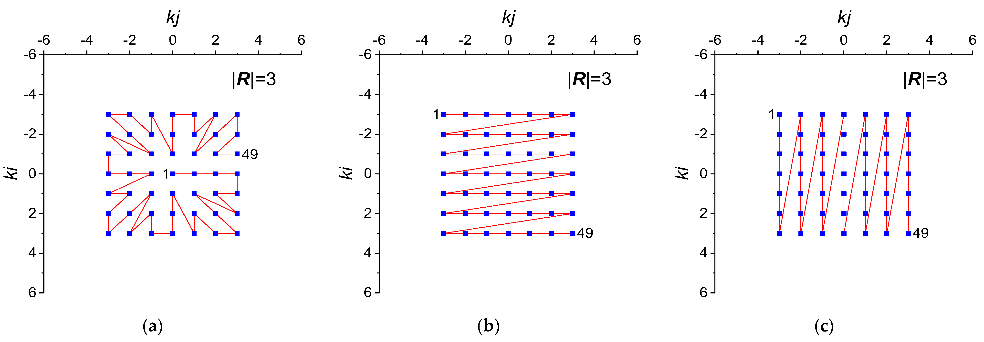
2.3. Method for Two-Dimensional NNetEn_2D Calculation with Square Kernels

As an alternative to circular kernels, we explored square kernels with three types of pixel enumeration. There are three version of square kernels: circular enumeration of pixels (SQCi_R), with enumeration by rows (SQRo_R) and by columns (SQCo_R), where the prefix ‘R’ is the radius of the circle inscribed in the kernel.

Examples of the three types of square kernels are shown in Figure 4.

The number of pixels N in a square kernel has a quadratic dependence on the radius N = (R·2 + 1)²; some cases are shown in

Table 3. Number of pixels N in a square kernel versus radius R.

R	1	2	3	4	5	6	7	8	9
N	9	25	49	81	121	169	225	289	361

.

It can be seen in Table 2 and Table 3 that the number of pixels of N square kernels and circular kernels can be the same, for example N(SQCi_3) = N(CIR_4) = 49 or N(SQCi_4) = N(CIR_5) = 81. This allows a better comparison of the effect of the kernel shape on the distribution of NNetEn_2D for these cases.

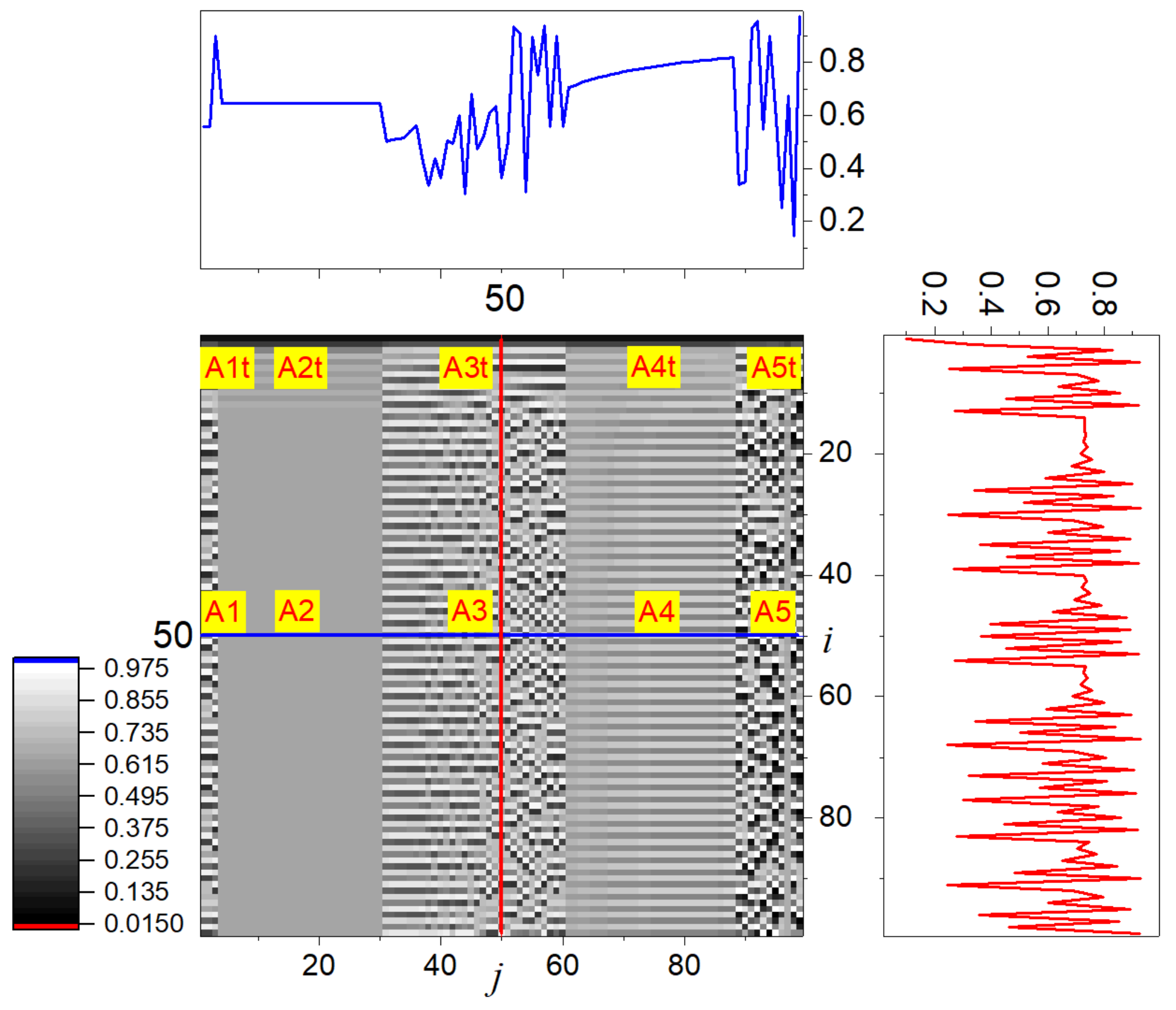
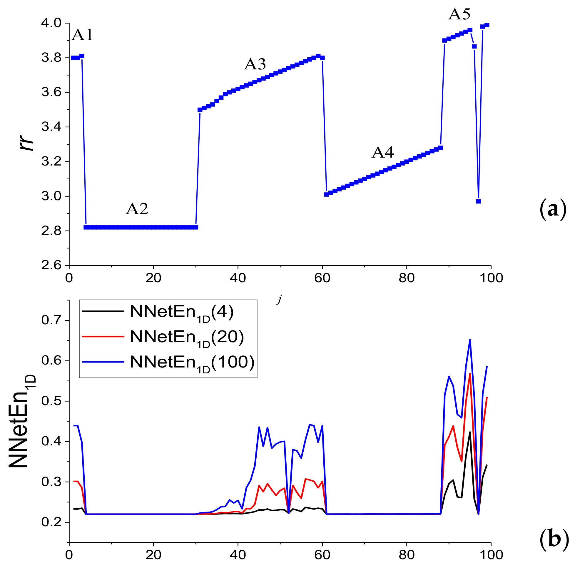
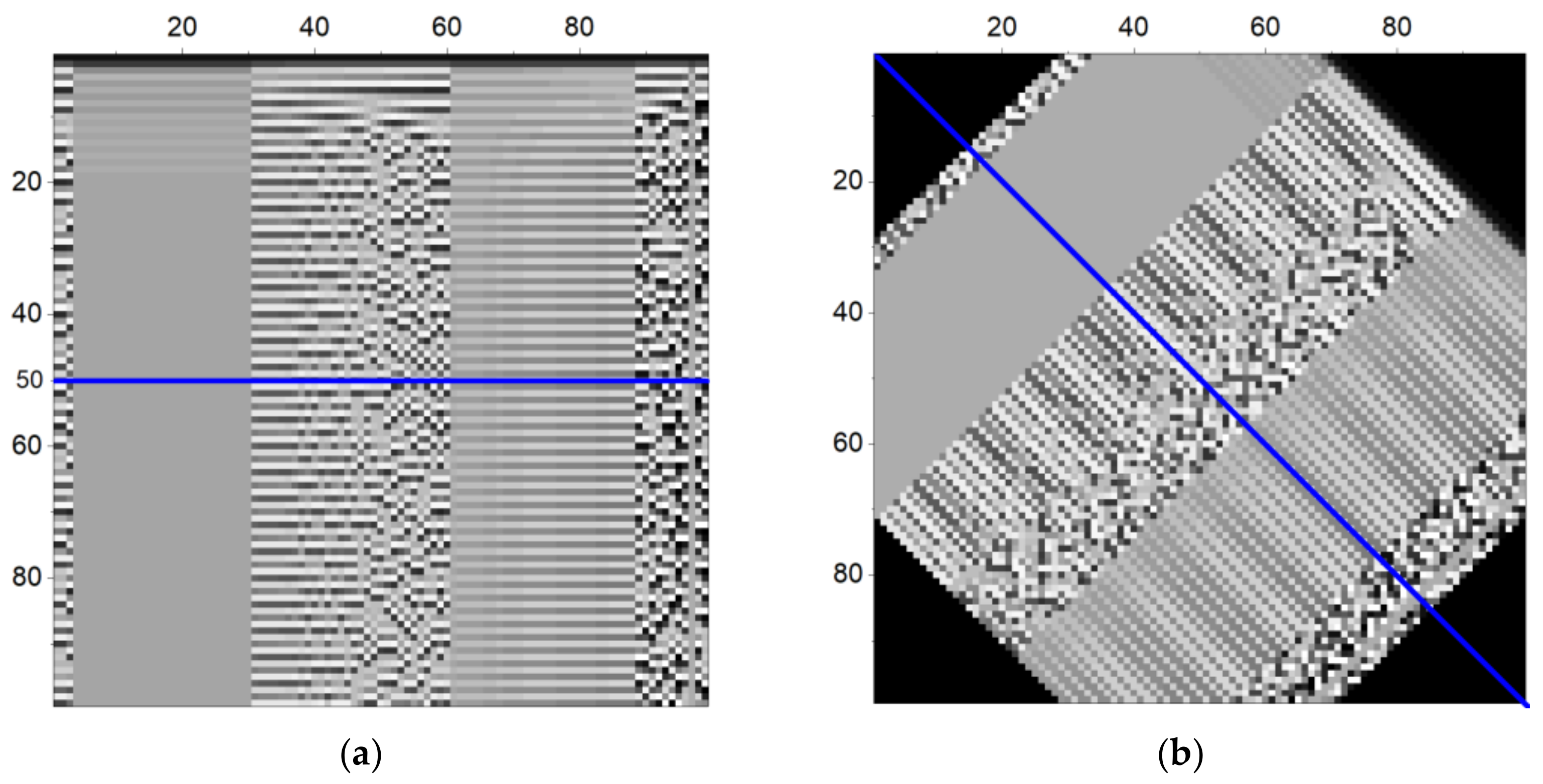
2.4. Artificial Test Image

The artificial test grayscale image is shown in Figure 5; it has a size of 99 × 99 pixels. The principle of its formation is based on the logistic mapping, according to which the pixel brightness B_i,j is modulated by a recursive function:

$$\left\{\begin{array}{l}{B}_{1,\mathrm{j}}=0.1\\ B_{\mathrm{i}+1,\mathrm{j}}=r{r}_{\mathrm{j}}\cdot B_{\mathrm{i},\mathrm{j}}\cdot (1-B_{\mathrm{i},\mathrm{j}}),i=1\dots 98\end{array}\right.$$

(5)

where the coefficient rr_j varies along the j axis in accordance with the dependence shown in Figure 6a. Such a dependence forms on the test image (Figure 5) areas with chaotic and ordered behavior and the main five areas are designated as A1–A5. In addition, there are areas where the logistic function has a transient mode; these areas are designated as A1t–A5t.

The most ordered behavior should be expected in the area of constant brightness A2 (4 ≤ j ≤ 30) and the area of uniform increase in brightness A4 (61 ≤ j ≤ 88). Chaotic behavior should be expected at the edges of the image (areas A1, A5), its center (A3) and transition regions (A1t–A5t). Figure 5 shows several sections along the axes j = 50 and i = 50. The NNetEn_1D calculation for the data series starting at i > 50 and length N = 49 is shown in Figure 6b. It can be seen that the entropy has an increased value in the regions (A1, A3, A5), which is a sign of chaotic behavior, and one should expect similar behavior from 2D entropy. It can be noted that even the use of a low number of epochs Ep = 4 when calculating NNetEn allows us to successfully identify areas of chaotic and ordered behavior. Using a reduced number of epochs allows faster calculations and can be useful in practice.

2.5. Image Preprocessing Methods

Pre-processing comprised removing the constant component from the images and rotating the images by different angles.

2.5.1. Removing the Constant Component of the Brightness of the Image

For a grayscale image, the calculation of entropy can provide more information if the constant component is removed from the array, according to the formula

$$B{\prime }_{\mathrm{i},\mathrm{j}}=B_{\mathrm{i},\mathrm{j}}-A$$

(6)

where A is a user-defined constant and B’ is a new array of pixel brightness. We used the average brightness value A = mean(B_i,j).

2.5.2. Image Rotation

For the rotation procedure, we used nearest neighbor resampling. This produces more pixelated results than bilinear or bicubic interpolation but does not affect the pixel values. This is especially important for the test image that would have been heavily distorted by interpolation.

Figure 7 shows two versions for the test image: the original and one rotated by 45° (clockwise). The image size of 99 × 99 provides rotational symmetry with respect to pixel number i = 50, j = 50.

Profile change during rotation was evaluated on a horizontal section i = 50 for the initial image, which transitioned to a diagonal section when rotated by 45° and a vertical section (j = 50) when rotated by 90° (see blue line in Figure 7).

It can be seen that the sections before and after the rotation by 45° do not completely coincide, since the values change as a result of averaging over pixels. The values best match in the areas of ordered behavior (A2, A4), and match the worst in the chaotic areas (A3, A5).

To evaluate the change in image profiles and the results of the NNetEn_2D calculation during rotation, the percentage change in profile (PCP) characteristic was introduced.

The initial and final profiles were given in a distance coordinate system, with the origin at the central pixel (i = 50, j = 50) (See Figure 8). Then, the profiles were divided into samples NK = 1000, k = 1…NK in the range of distances (−33 ≤ Distance ≤ 33), as shown in Figure 8, and in each sample the values of the initial profile (V0_k) and after rotation (V1_k) were estimated. The values of V0_k and V1_k were calculated using a linear approximation between known values.

PCP was calculated using the formula

$$\mathrm{PCP}=\frac{{\displaystyle \sum _k|V{1}_{\mathrm{k}}-V{0}_{\mathrm{k}}|}}{NK}\frac{1}{(V{0}_{\max }-V{0}_{\min })}\cdot 100\%$$

(7)

where V0_max is the maximum value of V0_k and V0_min is the minimum value of V0_k. To estimate the change in the image profile, the brightness value B_i,j was used as the V value. To estimate the entropy change during rotation, the NNetEn_2D value was used as the V value.

Rotating the image by 45 degrees (Figure 7) gives PCP = 4.4% for brightness. Rotating the image by 90 degrees gives PCP = 0%, which is expected, and indicates a complete match of the brightness profiles.

2.6. Main Steps for Estimating the NNetEn_2D of Images

On the basis of Section 2.1, Section 2.2, Section 2.3, Section 2.4 and Section 2.5 the main steps in the calculation of the NNetEn_2D are:

• Carrying out image preprocessing if necessary,
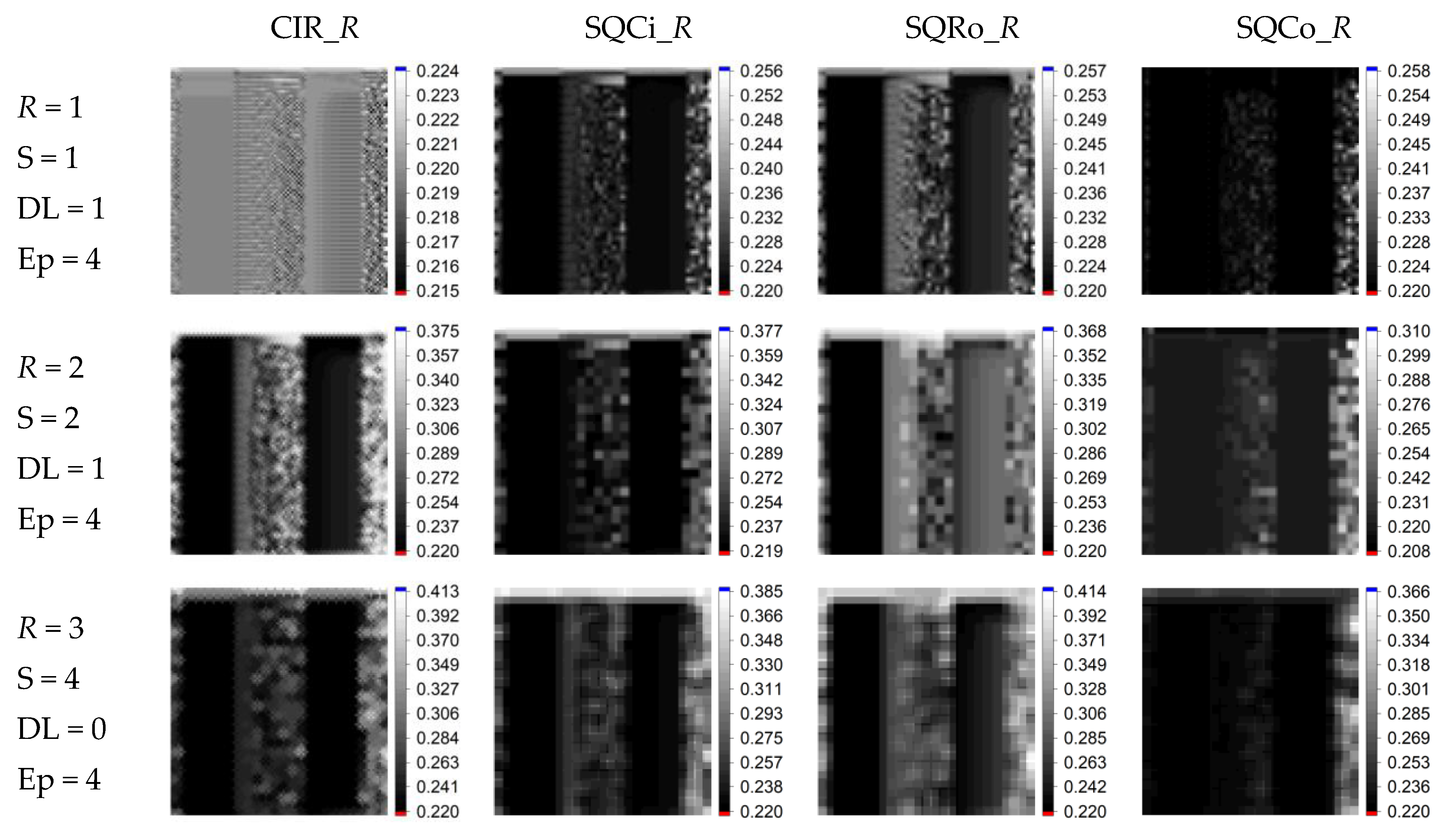
• Select kernel type (CIR_R, SQCi_R, SQRo_R, SQCo_R),
• Choose parameters R, S, DL, and division of the image area into circular kernels,
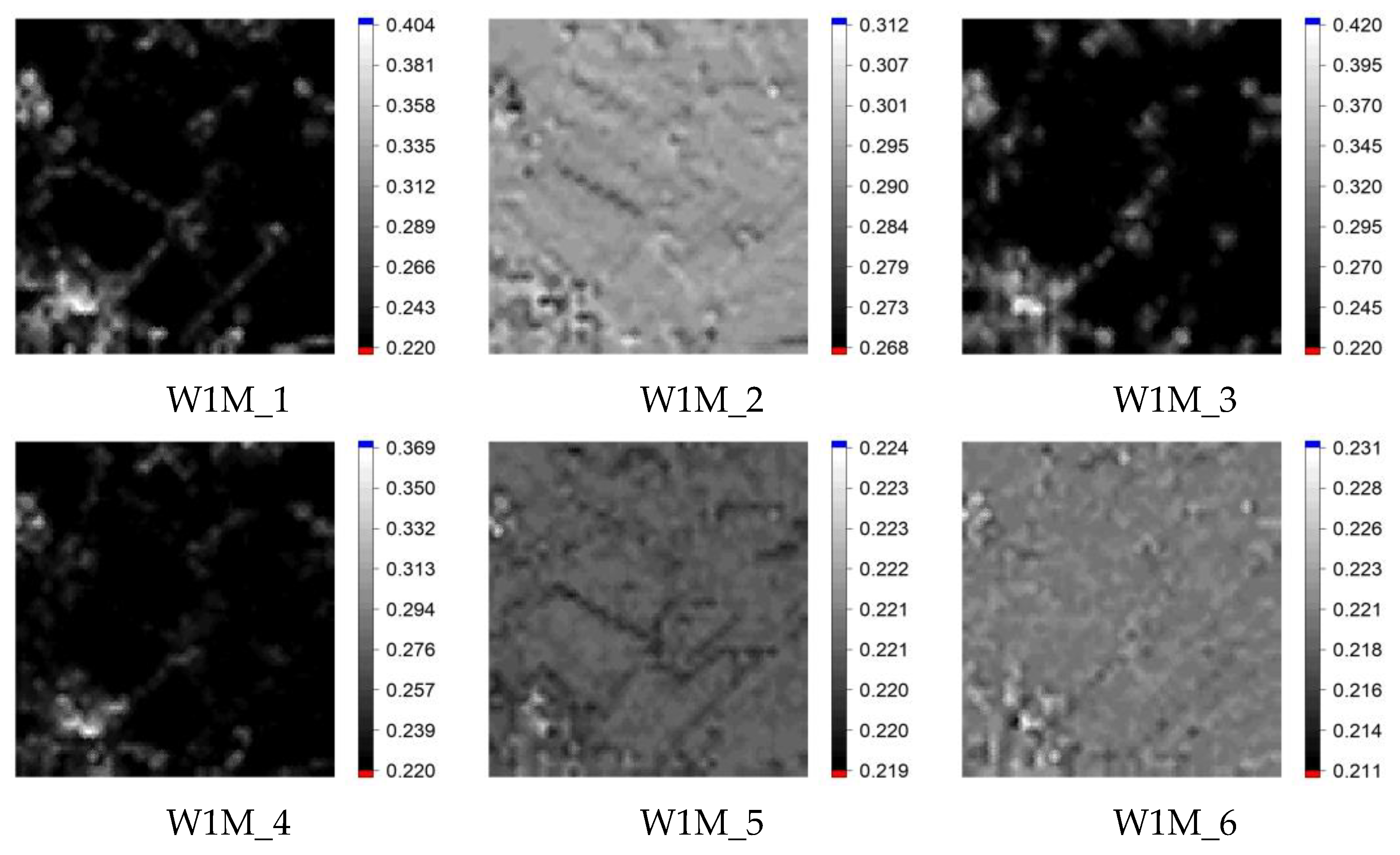
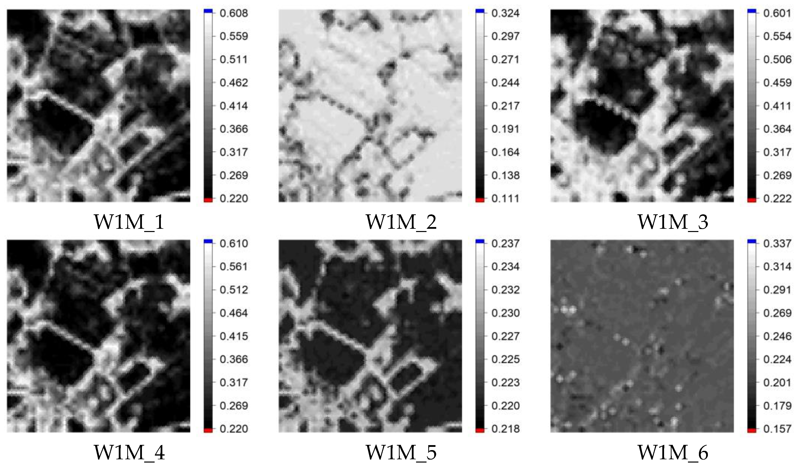
• Selecting the number of epochs Ep for calculating NNetEn_2D and techniques for filling the matrix (W1M_1-W1M_6),
• Calculation of NNetEn_2D in each spherical kernel,
• Calculate the resulting entropy for each pixel as the average of all NNetEn_2D from all kernels using that pixel.

Software for calculating NNetEn_2D can be downloaded in the Supplementary Materials.

3. Results

3.1. Research Results on the Test Image

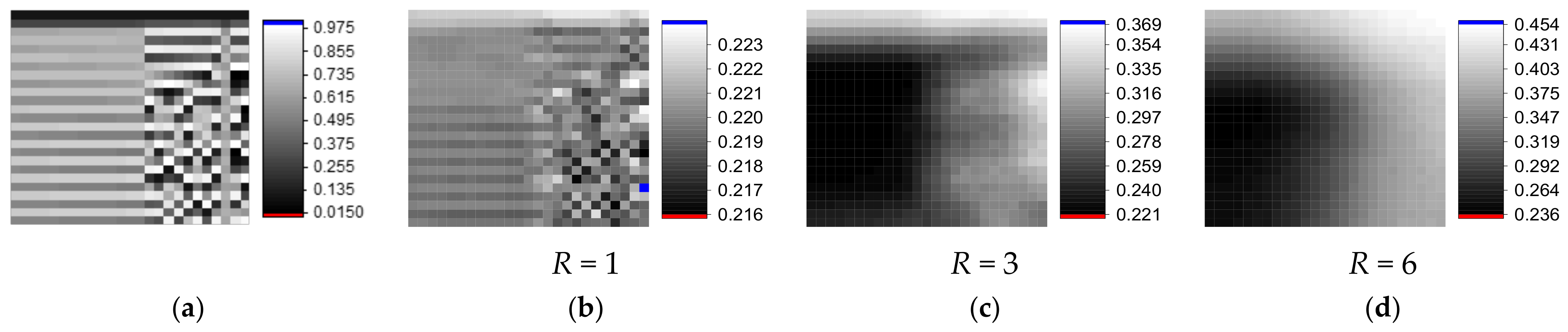
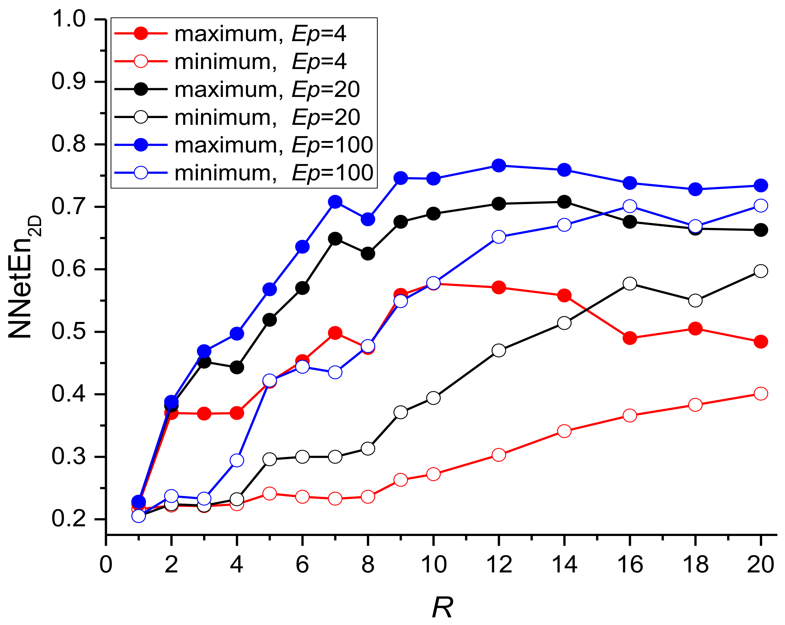
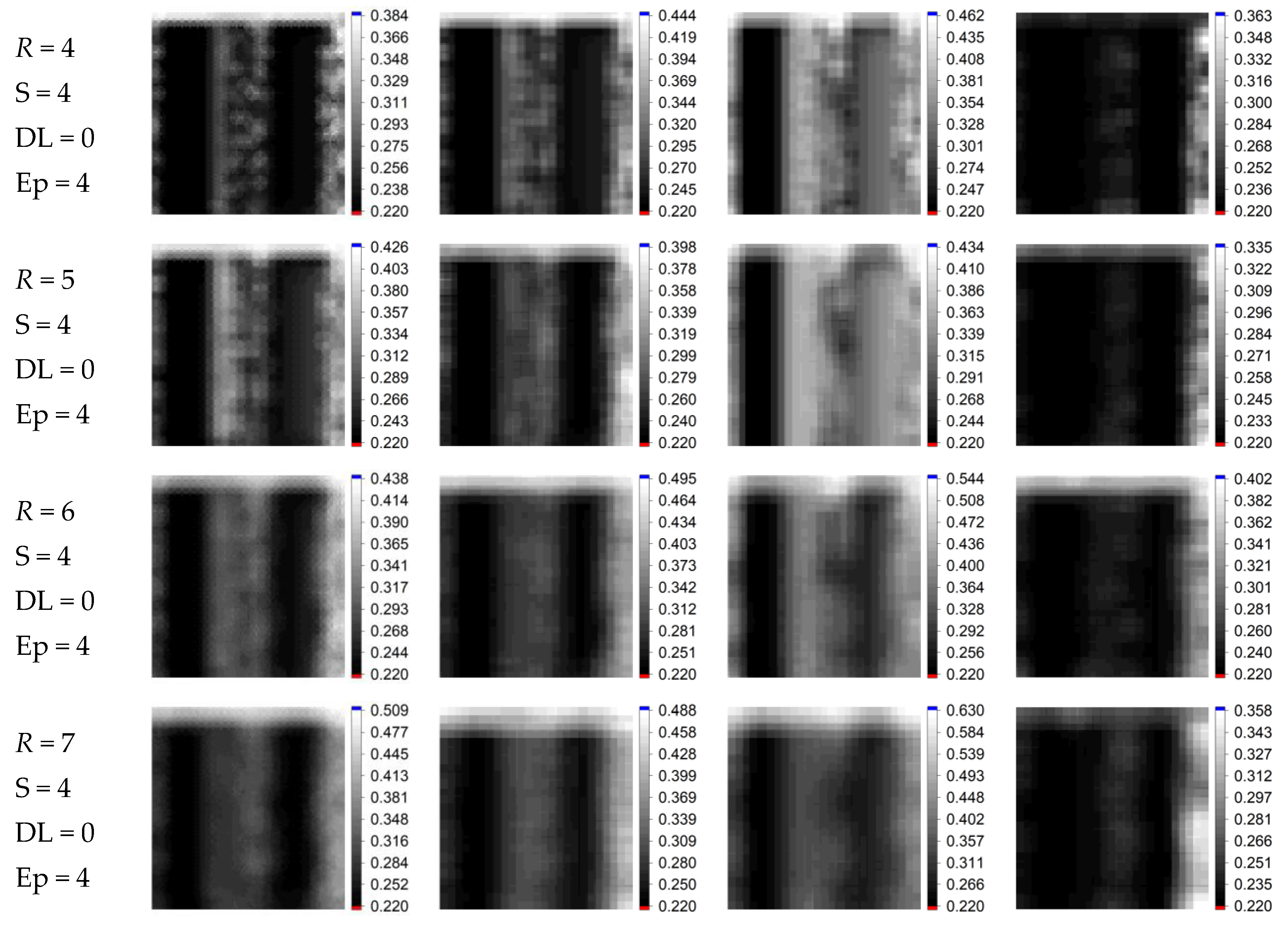
3.1.1. Effects of Kernel Radius and Number of Epochs on NNetEn_2D Variance

The dependence of the distribution of NNetEn_2D on the radius of circular kernels was studied on a test image area (A5t) with a size of 25 × 25 pixels (Figure 9a). The distributions of NNetEn_2D for various radii are shown in Figure 9b–d; black corresponds to the minimum value of NNetEn_2D and white corresponds to the maximum value of NNetEn_2D. Figure 10 shows the dependence of the maximum and minimum values of NNetEn_2D in the area under study depending on the kernel radius. It can be seen that as the radius increases, the sharpness of the NNetEn_2D distribution decreases, while the range of NNetEn_2D variation also changes.

As the radius increases, the maximum value of entropy increases, which is associated with an increase in the number of pixels in the kernel. Short data series of 2–15 elements do not give a high entropy value, since it is impossible to build a chaotic distribution using a small number of elements (see discussion section). With an increase in the radius to R = 5 and above, the number of elements in the data series increases N ≥ 81; as a result, the entropy value can reach maximum values. When the kernel diameter becomes comparable with the size of the picture (R ≥ 10), size effects begin to play a role, which are expressed by an increase in the minimum entropy value and a decrease in NNetEn_2D maximum value. This is due to the principle of mirroring pixels in areas outside the image, and the intersection of many pixels for kernels in different parts of the image. Thus, for the considered example, the widest range of NNetEn_2D corresponds to the radii R = 5–12.

An increase in the range of NNetEn_2D can also be achieved by increasing the number of epochs Ep. Figure 10 shows the dependences of the maximum and minimum values of NNetEn_2D for the number of epochs Ep = 4, 20, 100. It can be seen that the maximum range increases with the number of epochs. The choice of the number of epochs when calculating the entropy is user dependent; a lower number of epochs ensures faster algorithm operation. In practical implementation, a low number of epochs, Ep = 4 or Ep = 20, provide a reliable spatial separation of the regular and chaotic behavior of 2D data.

3.1.2. NNetEn_2D Distribution Examples for Different Kernels

Examples of the distribution of NNetEn_2D for different types of kernels are shown in Figure 11. The first column corresponds to circular kernels (CIR_R), the rest correspond to square kernels SQCi_R, SQRo_R, and SQCo_R. In general, all the kernels correctly identified chaotic areas A1, A3, A5, and A1t–A2t, which have an increased value of NNetEn_2D compared to regions with ordered dynamics A2 and A4. The results of circular and square kernels with circular filling symmetry CIR_R and SQCi_R have similar distributions. This is especially noticeable in examples with the same number of pixels in N kernels. For example, the distribution of CIR_4 is similar to SQCi_3, where N = 49 and CIR_5 is similar to SQCi_4, where N = 81. Distributions with SQCo_R have a low contrast in the chaotic central area (A3), and SQRo_R, on the contrary, has a high contrast in A3. Using CIR_R and SQRo_R allows areas A2 and A4 to be effectively separated, while other kernels fare worse at this task. According to our interpretation, the best representation of dynamics in the test pattern with sufficient image sharpness is given by kernels with radii of 4–6.

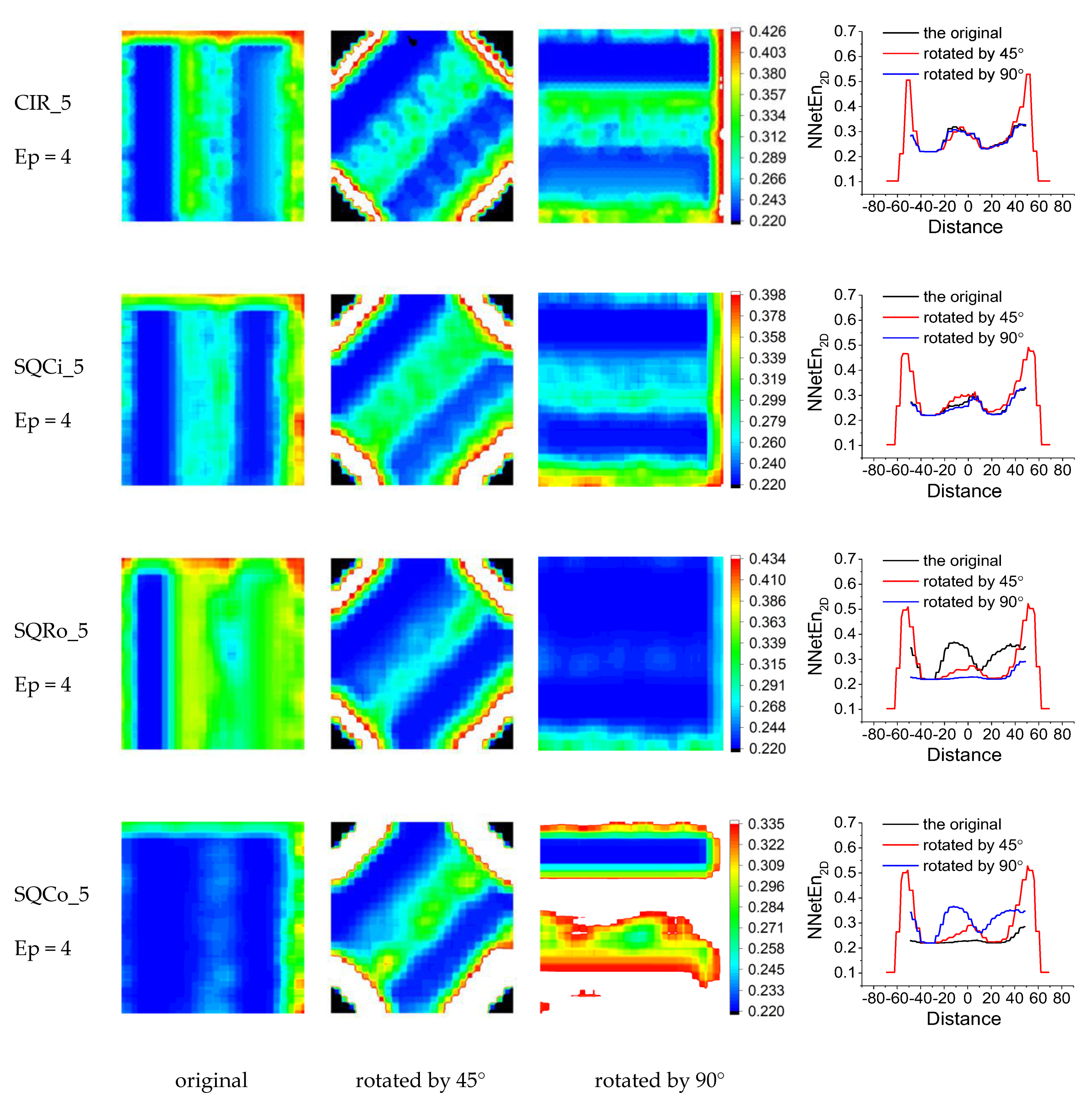
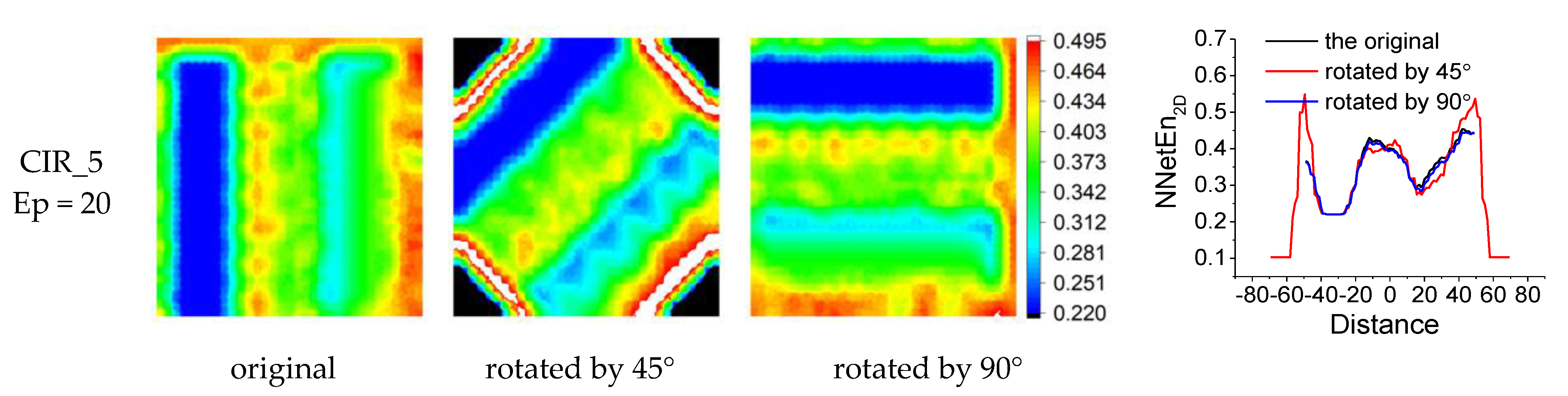
3.1.3. Effects of Image Rotation on the NNetEn_2D Distribution

The PCP calculation results for NNetEn_2D at rotations by 45° and 90° are shown in

Table 4. PCP for NNetEn_2D at rotations by 45° and 90° (Ep = 4).

PCP (%)	R = 1	R = 2	R = 3	R = 4	R = 5	R = 6	R = 7
kernel	PCP (%) for NNetEn2D when rotated by 45°
CIR_R	18.9	12.1	22.3	14.2	9.6	9.9	11.6
SQCi_R	12.2	16.1	21.6	14.7	15.7	29.3	25.3
SQRo_R	27.0	42	26.2	37.2	45.8	24.1	27.4
SQCo_R	34.9	101.9	107.2	113.2	169.7	105.7	98.3
	PCP (%) for NNetEn2D when rotated by 90°
CIR_R	12.9	10.5	10.9	8.7	4.3	3.9	6.1
SQCi_R	8.1	11.4	12.5	7.3	7.6	3.2	3.2
SQRo_R	34.0	45	33.4	51.6	57.2	43.9	48.6
SQCo_R	115.9	322.7	164.4	301.1	704.9	163.5	180.9

. The smaller the PCP, the smaller the change in the profile during rotation and the better the method. The best result was shown by the method using circle kernels CIR_R, the worst was for SQCo_R kernels. For CIR_5, PCP = 9.6% and for SQCo_5, PCP = 704.5%.

View of NNetEn_2D distributions with profiles for different type of kernel are shown in Figure 12.

For images rotated by 45° using CIR_5, we observe good profile repeatability in the central part of the image and increased entropy values at the border. This effect can be attributed to an artifact; it is associated with zero entropy values outside the picture, where mirror symmetry has not been implemented. For images rotated by 90° for circular CIR_5 kernels, we see good repeatability of NNetEn_2D profiles over the entire cross section range. The use of square kernels leads to a significant distortion of the entropy profiles during the rotation operation.

Table 5. PCP for NNetEn_2D at 45° and 90° rotation at different epoch numbers.

PCP (%)	R = 1	R = 2	R = 3	R = 4	R = 5	R = 6	R = 7
kernel type	PCP (%) for NNetEn2D when rotated by 45°
CIR_R, Ep = 4	18.9	12.1	22.3	14.2	9.6	9.9	11.6
CIR_R, Ep = 20	18.9	13.4	9.3	17.1	8.4	9.2	18
CIR_R, Ep = 100	18.9	9.5	7.4	10.4	7.8	4.1	12.2
	PCP (%) for NNetEn2D when rotated by 90°
CIR_R, Ep = 4	12.9	10.5	10.9	8.7	4.3	3.9	6.1
CIR_R, Ep = 20	12.9	13.8	6.3	10.1	3.1	1.5	1.5
CIR_R, Ep = 100	12.9	16.3	6.9	7.6	1.5	1.2	4

shows the results of calculating the PCP with a variation in the number of epochs Ep, using the CIR_R circular kernels.

It can be seen that there is a tendency for PCP to decrease with increasing Ep for kernels with radius R = 5 and R = 6. Thus, by choosing the values of R and Ep, one can achieve a smaller value of PCP, thereby reducing the effect of the rotation operation on the entropy distribution. As an example, Figure 13 shows the distributions of NNetEn_2D for Ep = 20, where the profiles almost completely coincide after rotation by 90°.

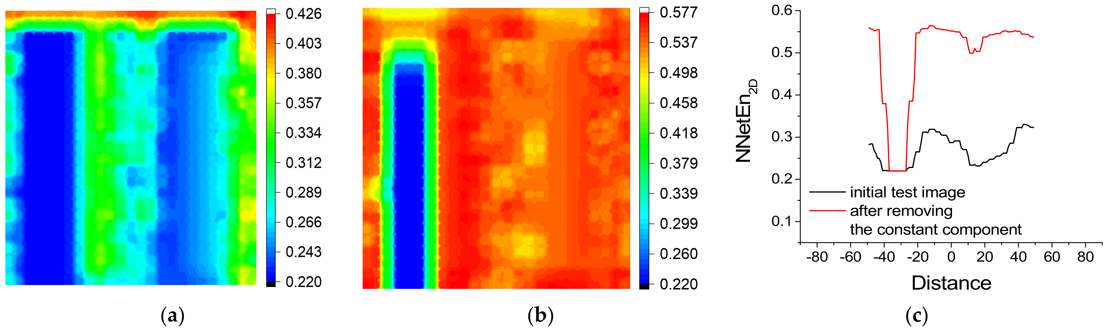
3.1.4. Effects of Removing Constant Component on the NNetEn_2D Distribution

Figure 14 shows the result of NNetEn_2D calculation before and after removing the constant component of image brightness. It can be seen that the removal of the constant component increased the range of change in NNetEn_2D, while some areas increased in contrast (for example, (A2)), others decreased (A3). Thus, preprocessing allows us to see the distribution of entropy in a different contrast and can be useful in practice.

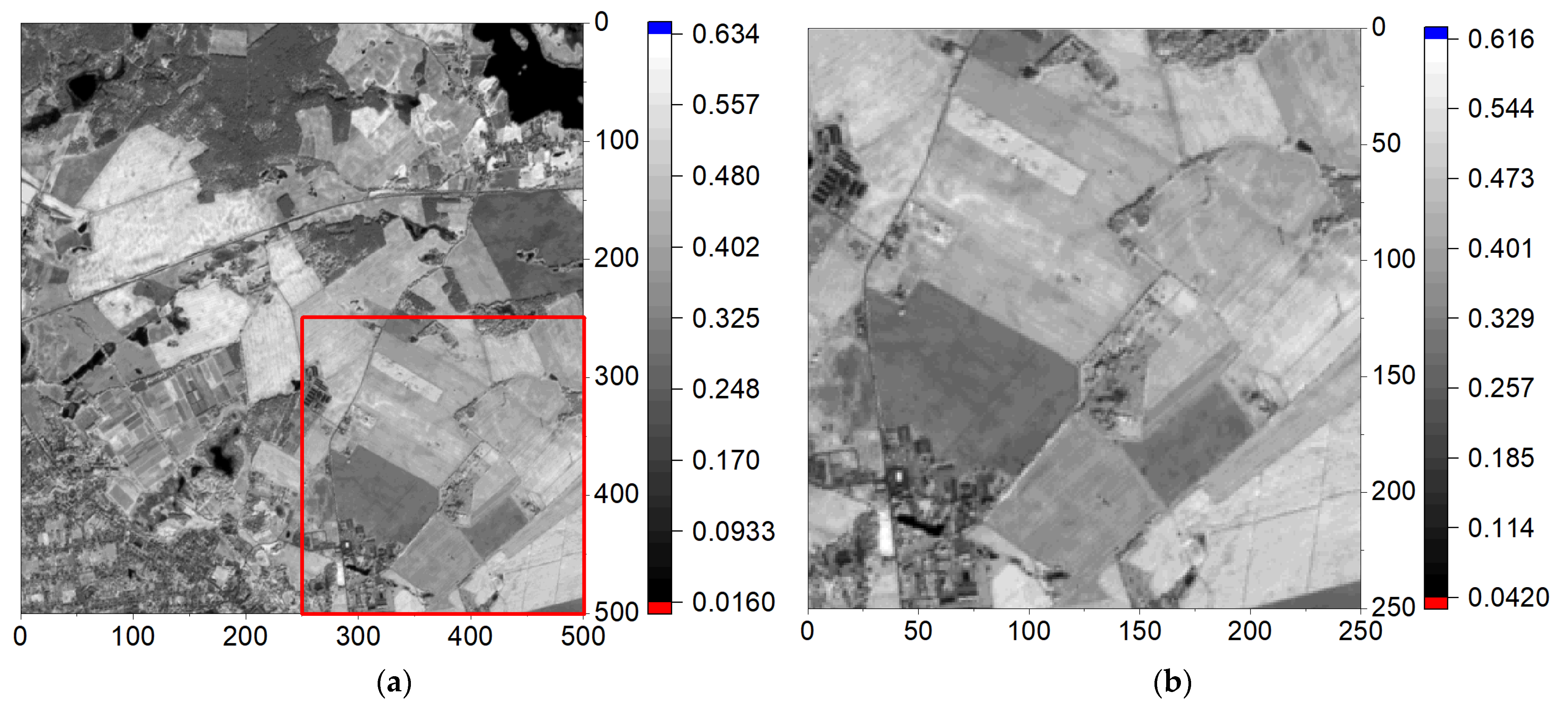
3.2. Results of the Study on Sentinel-2 Images

We selected five images of a region in Brandenburg, Germany. The subset was chosen to represent a variety of different land cover types, including croplands, forests and urban areas, as well as water bodies. The images (Sentinel-2) were acquired between March and August 2018, illustrating varying conditions throughout the main growing season. The size of the studied images was 500 × 500 pixels.

In Section 2.6, the main steps in calculating the entropy of NNetEn_2D were given. The calculation result mainly depends on the choice of calculation parameters, which include: image preprocessing method; kernel type (CIR_R, SQCi_R, SQRo_R or SQCo_R); parameters R, S, DL; number of epochs Ep; and techniques for filling the matrix (W1M_1-W1M_6).

Based on the results of Section 3.1, the following parameters were chosen: kernel type CIR_5, R = 5, S = 6, and DL = 1. The choice of step S is determined by the size of the image and the radius of the kernel. A minimum step S = 1 drops the entropy calculation speed, so S = 6 is the compromise value. Number of epochs Ep = 4.

It is necessary to determine the preprocessing method and the technique of filling the matrix (W1M_1-W1M_6). The preprocessing method has two options: (1) use the original data or (2) subtract the constant component from the data according to the method in Section 2.5.1. In the next section, we will show the preliminary results of the calculation by varying these parameters and choosing the best combinations.

3.2.1. Effects of Data Preprocessing on the NNetEn_2D Distribution

Figure 15a shows an image from a satellite (Sentinel-2) with a size of 500 × 500 pixels and a constant component A = 0.348320. Figure 15b shows a subset of the main image (highlighted with a red frame), 250 × 250 pixels in size.

Figure 16 shows the result of calculating NNetEn_2D for the initial data for the subset, using all techniques for filling the reservoir matrix (W1M_1-W1M_6).

It can be seen that the application of the W1M_1, W1M_3 and W1M_4 techniques to the initial subset leads to a greater selection of boundaries and a weak contrast of the entropy of the remaining regions. The result of applying the W1M_2, W1M_5 and W1M_6 techniques does not lead to an obvious delimitation of areas according to features, with a narrow range of entropy changes.

Figure 17 shows the result of calculating NNetEn_2D for the initial data for the subset from which the constant component A = 0.348320 has been removed, using all techniques for filling the reservoir matrix (W1M_1-W1M_6).

The application of the W1M_1, W1M_3 and W1M_4 techniques to the initial subset from which the constant component is removed (Figure 17) shows, in our opinion, the best results in highlighting areas of chaos and order and a wide range of entropy changes. The result of applying the techniques W1M_2, W1M_5 and W1M_6 leads to the identification of areas with only high entropy and a narrow range of entropy changes.

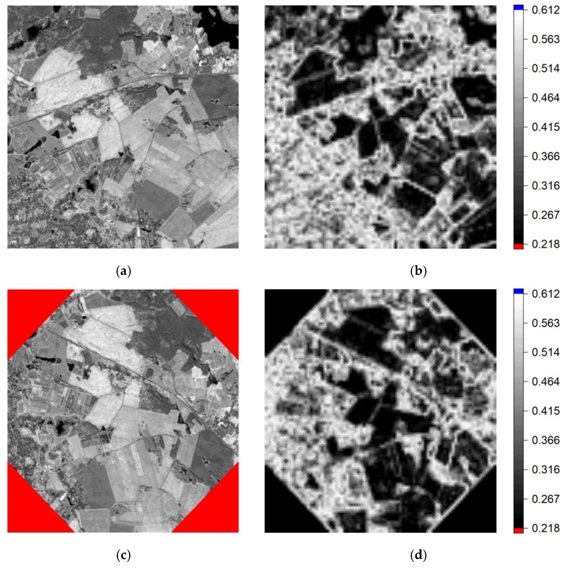
3.2.2. Effect of Image Rotation on the NNetEn_2D Distribution

Figure 18d shows the entropy calculation result after rotating the image by 45° (original in Figure 18a). It can be seen that NNetEn_2D quite accurately repeats the result in Figure 18b. This, once again, confirms the operability of the method of using circular kernels.

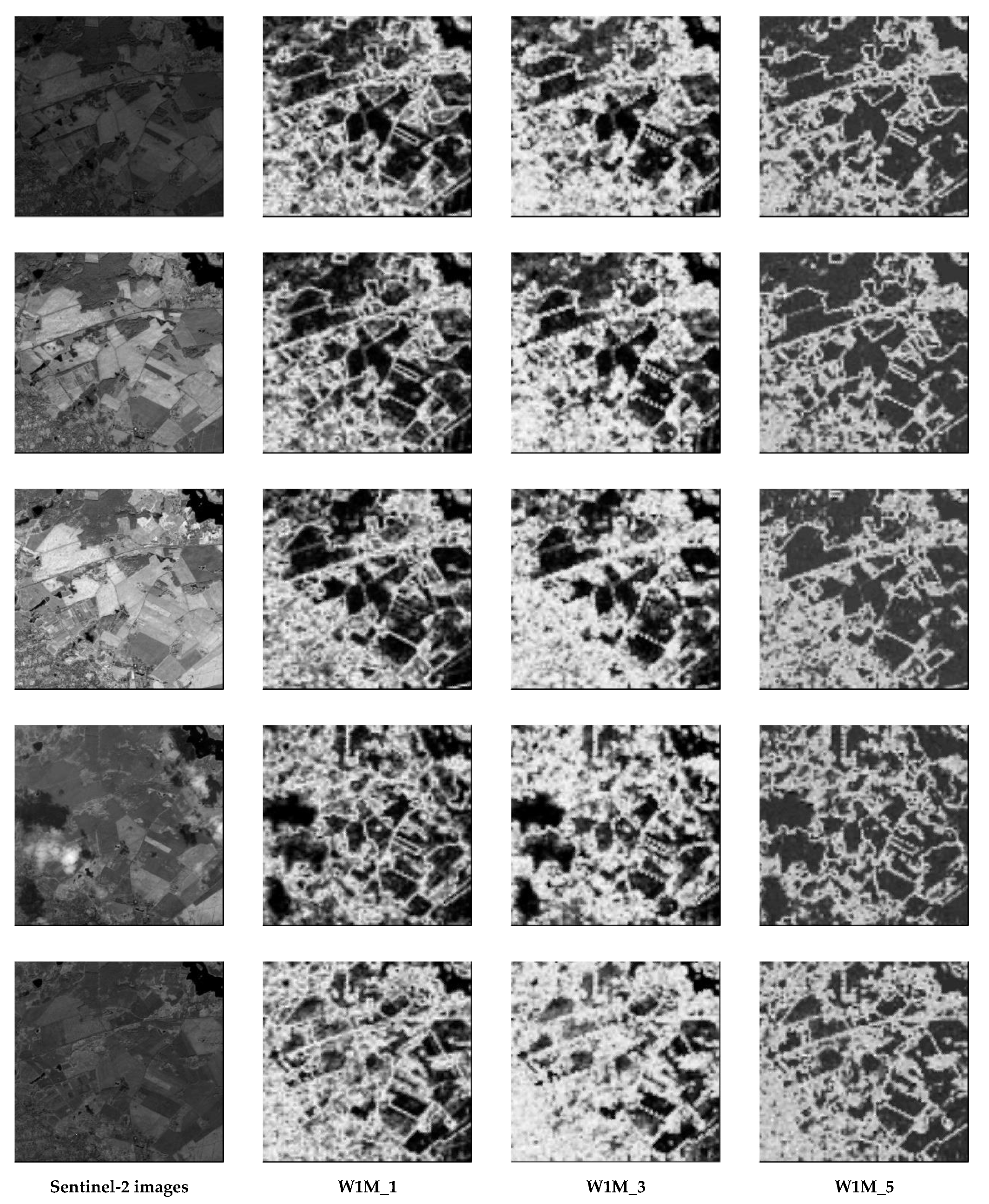
3.2.3. NNetEn_2D Distribution of Sentinel-2 Images

In Figure 19, we compare results of the new method using different matrix filling schemes, after subtracting the constant component. In general, it can be seen that the entropy characterizes the structure of the Sentinel-2 scenes quite well. Areas of sharp transitions (e.g., between fields and urban areas) have high entropy values, while more homogeneous areas have consistently low values (e.g., water bodies, top right). Brightness changes in the images throughout the growing season do not affect the entropy results with homogeneous fields appearing dark throughout time. Even different types of forests (top left) seem to be distinguishable. An interesting effect is that both clouds and cloud shadows lead to consistently low entropy values, highlighting a potential of using this technique for cloud and shadow detection. These characteristics indicate the success of NNetEn_2D in providing meaningful entropy information for 2D imagery.

Regarding different filling methods, Figure 19 indicates that W1M_1 and W1M_3 lead to clearer results with higher contrast than W1M_5. W1M_1 seems to best capture local heterogeneities while W1M_3 tends to create a blurrier picture with less distinct features.

In Figure 20, we show results of the NNetEn_2D and GLCM entropy. This illustrates the superior performance of the new method in distinguishing heterogeneous from homogeneous image areas to form a more coherent picture of the conditions. While water bodies are clearly visible in GLCM entropy, also with constantly low values, homogeneous fields especially are less clearly separated and borders between objects are expectedly much less precise.

Another observation is that results of GLCM entropy are not affected by subtracting the constant component of the image. Since calculation of GLCM first involves a quantization of pixel values, most commonly based on evenly spaced thresholds or by evenly distributing pixel values across bins, a constant change applied to all pixels indiscriminately does not affect the distribution after quantization.

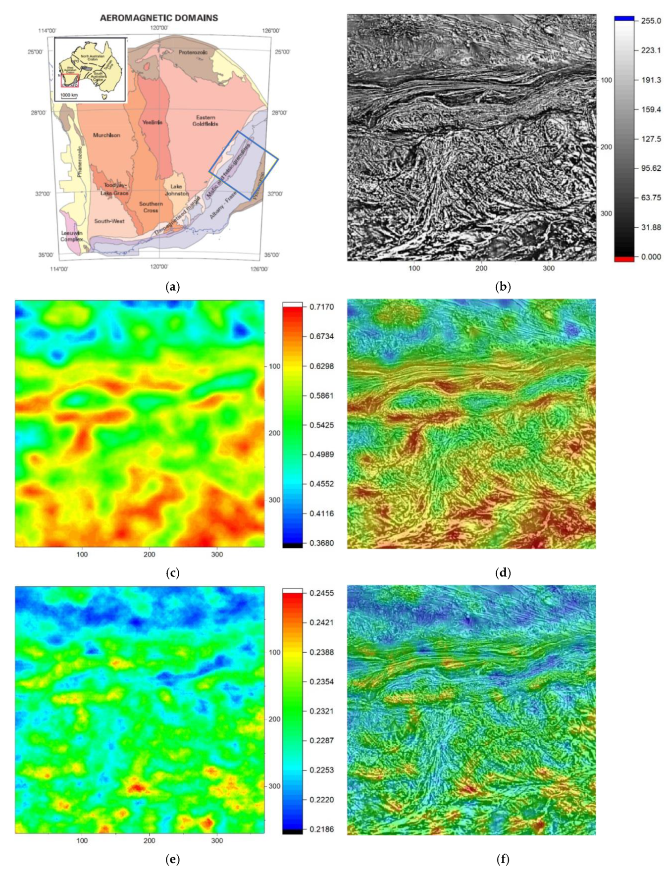
3.3. Research Results on Aero-Magnetic Images

As an example of a geophysical image, we selected an area (Figure 21a) from southwest Australia [31]. The aeromagnetic image is shown in Figure 21b and is extracted from [32]. The entropy images are shown in Figure 21c. In particular, Figure 21d shows Figure 21c draped over the aeromagnetic image. The geophysical structure is amplified in this image and confirms the geophysical mapping that shows that the rocks to the north-west, characterized by low to medium entropy, also occupy the core of the fold in the northeast of the area and also occur further to the south. This kind of information would be very useful prior to undertaking field mapping.

When using the W1M_6 technique for filling the matrix, the NNetEn_2D distribution takes the form shown in Figure 21e. The entropy distribution in this case similarly labels regions of high and low entropy, but with less contrast. The entropy range in Figure 21c is NNetEn_2D (0.368…0.717) and in Figure 21e is NNetEn_2D (0.218…0.245). This distribution confirms the conclusions made above, but may be more preferable for the visual perception of the results.

4. Discussion

In this paper, two criteria for the quality of the methodology are proposed. First, a test image was generated that used the logistic mapping (Equation (5)), for which the areas of chaos and order are known depending on the control parameter rr. It is shown that our method correctly identified chaotic areas A1, A3, A5, A1t–A2t, which have an increased value of NNetEn_2D compared to regions with ordered dynamics A2 and A4 (see Figure 11 and NNetEn_2D profiles Figure 12 and Figure 13). In addition, NNetEn_2D for area A5 is larger than for area A3 (kernel type CIR_R), which repeats the dependence for one-dimensional entropy in Figure 6. However, there is a big difference between the profiles of the one-dimensional and two-dimensional tasks, since the irregularity of the two-dimensional distribution is due to the irregularity along two axes. The second quantitative criterion is the calculation of the PCP characteristic (Equation (7)), which clearly shows the best shape of kernel invariant to rotation.

The best results were obtained with kernels of circular symmetry CIR_R; the advantage was the greater invariance of the result when the image was rotated. However, square kernels are also able to distinguish regions of chaos and order, and for the same number of pixels, can give similar distributions to circular kernels such as SQCi_3 and CIR_4.

This property can be used to replace circular kernels with square kernels for rough calculations. Square kernels are in general much easier to implement and often more efficient to execute in many programming languages (e.g., Python, Delphi or MATLAB), so their consideration may be of practical interest to researchers. In addition, it is of interest to compare the result of NNetEn_2D calculation after the operation of rotating the image for different types of kernels.

The best performance for the test pattern was shown by kernels with radii R = 5 and R = 6 pixels; low PCP values were observed for them, not exceeding 10% for Ep = 4 (Table 5), and a wide range of entropy (Figure 10). For kernels with a small radius R = 1–3, the entropy range narrowed significantly. For R = 1, the maximum and minimum values of NNetEn_2D practically coincided; PCP~18% in this case also has higher value. The low range of NNetEn_2D for small radii is due to the fact that short data series do not give a high entropy value, since it is impossible to build a chaotic distribution on a small number of elements. Figure 10 shows that the entropy range can also be expanded by increasing the number of epochs Ep; this is due to the training effect of the LogNNet neural network. A larger number of epochs leads to a greater degree of classification of LogNNet and, accordingly, an increase in NNetEn_2D; this effect is demonstrated in Figure 6b.

From Table 5, one can see the effect of decreasing PCP for entropy with an increasing number of epochs Ep for radii R = 5 and R = 6, PCP can reach very low values (~1.2%) when the pattern is rotated by 90°. For radius R = 1, the PCP values do not change with the number of epochs, which indicates that the limiting values of NNetEn_2D quickly reach the limit in the case of small values of the number of elements in the kernel.

Thus, for a reliable determination of the entropy, it is preferable to use R ≥ 4. The selection of the radius in each specific case is the task of the user. For example, with artificial scaling of images, the pixel density changes and, therefore, it is necessary to select the optimal radius individually.

The NNetEn_2D entropy calculation method has two main geometric parameters (kernel radius and its displacement step), as well as two parameters of neural network (number of training epochs and one of six reservoir filling techniques). The choice of these parameters determines which features of the image will be highlighted to a greater extent.

With almost any transformation of the image, including rotation, changes to the location and values of pixels in the work, it was calculated that a rotation by 45° leads to a value of PCP = 4.4% for brightness. NNetEn_2D is a sensitive tool for detecting these changes. Therefore, in Figure 12 for the CIR_5 kernel, the formation of alternating stripes in the center of the figure is seen. Similar stripes are also observed in Figure 7b, but their contrast is very weak. Thus, the calculation of NNetEn_2D makes it possible to reveal hidden changes when the image is rotated or modified in some other way.

Figure 16 and Figure 17 show that modifying the constant component of 2D data significantly affects NNetEn_2D. NNetEn is a value that determines the measure of data disorder relative to the zero level. For example, a signal in the form of weak noise against the background of a high constant component has a low entropy, but when the constant component is removed, the remaining noise, on the contrary, has a high entropy. Therefore, data preprocessing is an important step in NNetEn_2D calculations and allows focusing on certain phenomena of the chaotic dynamics of 2D data.

In our tests on remote sensing imagery, the method demonstrates capacity to represent entropy accurately in different image parts. Heterogeneous areas (sharp transitions, strong texture) are consistently highlighted, while homogeneous areas have very low entropy values. In particular, the consistent highlighting of both clouds and cloud shadows may prove advantageous in the future. Although results are encouraging, remote sensing applications would benefit significantly from a more detailed, pixel-wise application rather than the large kernel averaging that was applied in this study. However, the high processing requirements of the technique make this very difficult, for now. Therefore, further research will be focusing on increasing efficiency, as well.

The comparison with GLCM further revealed advantages but also disadvantages of this early version of the technique. On the one hand, results are of significantly higher quality and consistency, but on the other, the effect of the constant component on results needs further analysis to gather real-world guidelines.

As far as the aeromagnetic image (Figure 21b) is concerned, the patterns arise from different distributions of magnetic susceptibility in the rock and their interaction with the Earth’s magnetic field. The mineral responsible for the magnetic susceptibility is mainly magnetite. Metamorphism at high temperatures and pressures along with plastic deformation distributes the magnetite in patterns that derive from deterministic processes (reaction–diffusion). Hence, the entropy is saying something about these processes and the complexity associated with them. The choice of the kernel radius R, the technique of filling the matrix (W1M_1-W1M_6) and the value of Ep allow one to select favorably certain features of the NNetEn_2D entropy for further analysis.

The task of increasing the speed of NNetEn_2D entropy calculation is important. At the moment, calculating an area of 99 × 99 pixels takes about 9 min, and larger areas of 500 × 500 pixels require about 200 min of computing time using the 30 threads of an AMD Ryzen 9 3950× 16-core processor with 64GB of RAM.

To estimate the computational cost, it is convenient to introduce a vector C with components expressing the number of addition and subtraction operations N(±), multiplication operations N(*), division operations N(/) and exponential operation N(exp), C = (N(±), N(*), N(/), N(exp)). In vector C, we only consider mathematical operations and do not take into account the operations of extracting and writing data to memory.

Table 6. Computational cost of the main stages of the NNetEn_2D calculation algorithm.

Stage Number	Stage Description	Vector of Computational Cost C = (N(±), N(*), N(/), N(exp))
1	Multiplication of the W1 matrix by the Y vector in the reservoir (see Figure 1)	C1 = (19,625, 19,625, 0, 0)
2	Normalization of the vector Sh	C2 = (100, 0, 25, 0)
3	Forward method of the output neural network, multiplication of the matrix W2 by the vector Sh	C3 = (260, 260, 0, 0)
4	Normalization of the vector Sout	C4 = (10, 0, 10, 10)
5	Back-propagation method	C5 = (280, 540, 0, 0)
6	LogNNet training on one image	C6 = C1+ C2+ C3+ C4+ C5 C6 = (20,275, 20,425, 35, 10)
7	LogNNet training using 60,000 MNIST images	C7 = C6·60,000 C7 = (1.2165 × 109, 1.2255 × 109, 2.1 × 106, 6 × 105)
8	LogNNet training using Ep = 4 epochs	C8 = C7·Ep C8 = (4.866 × 109, 4.902 × 109, 8.4 × 106, 2.4 × 106)
9	LogNNet testing on one image	C9 = C1+ C2+ C3+ C4 C9 = (19,995, 19,885, 35, 10)
10	LogNNet testing using 10,000 MNIST images	C10 = C9·10,000 C10 = (1.9995 × 108, 1.9885 × 108, 3.5 × 105, 1.0 × 105)
11	NNetEn2D entropy calculation for one kernel	C11 = C8+ C10 C11 = (5.0660 × 109, 5.1009 × 109, 8.75 × 106, 2.5 × 106)
12	Calculation of entropy for one image sized 99 × 99 pixels, with parameters S = 6, R = 5. 324 circular kernels are needed to cover the entire image	C12 = C11·324 C12 = (1.6414 × 1012, 1.6527 × 1012, 2.835 × 109, 8.1 × 108)

presents the main stages of the calculation algorithm, with their brief description and evaluation of the vectors C. The vector index corresponds to the stage number.The basic operations are the first five stages with vectors C₁–C₅; they are repeated at the stages of training C₈ and testing the C₁₀ neural network.

The total computational cost for a single kernel C₁₁ contains a huge number of mathematical operations ~10⁹. To calculate an image of 99 × 99 pixels, the computational cost of C₁₂ is required, where the number of multiplication operations reaches ~10¹². Let us estimate the calculation time approximately. To do this, we first estimate the time to execute each operation included in the vector C, in relation to real numbers, taking into account the extraction and writing of values to a memory cell.

For a 1.61 GHz processor, the estimates give the following values: addition t(±) = 3.56 ns, multiplication t(*) = 6.04 ns, division t(/) = 8.22 ns, and exponent t(exp) = 71 ns. As a result, it is easy to estimate the total time T = N(±)·t(±) + N(*)·t(*) + N(/)·t(/) + N(exp)·t(exp) for C₁₂—it is T~265 min. In this work, we used parallel calculations into 30 threads at stage 12, which gives a correct estimate of the experimentally observed time of about 9 min.

The problem of high computational costs is a common problem of neural networks, in particular deep learning networks applied to individual pixels of an image. Specialized libraries such as TensorFlow or PyTorch are optimized for the efficient use of GPUs and parallel computation.

The present algorithm has the disadvantage that the computational cost is independent of the number of elements in the data series. A series with the N = 50 or N = 19,625 will be calculated in the same time, since the dimension of the reservoir matrix W₁ does not change. Let us compare the computational cost for another well-known method for calculating the approximate entropy (ApEn). In the ApEn [33] calculation algorithm, the number of operations grows quadratically, ~N², and reaches about 10⁹ at N = 19,625, which is comparable to the computational cost of NNetEn_2D at stage 11 in Table 6.

NNetEn_2D calculation time reduction can be achieved by reducing the computational cost and through parallel computing.

We can suggest the following methods of parallel computing:

• Parallelize the calculation of the product of a matrix and a vector in steps 1 and 3; this can increase speed up to 10–100 times.
• Organize a parallel calculation of the entropy for each image kernel at step 12. For the example shown in the Table 6, the acceleration will be 324 times.

Reducing the computational cost can be achieved by modifying the methodology and architecture of the neural network. The following paths can be suggested:

• Reduce the number of training images in step 7.
• Reduce the number of test images in step 10.

Further exploration of our technique in this direction will be the subject of further research.

The grayscale image (Figure 15a) is a set of pixels B_i,j. Suppose there is a need to process color images. The data for the three color channels (R, G, B) will represent three arrays RB_i,j, GB_i,j, and BB_i,j. In this case, we will offer three options for calculating NNetEn_2D: (1) for each color channel separately, (2) converting a color image to grayscale, and (3) concatenate data for three colors. In the future, we plan to further explore the potential of this method in remote sensing applications, including the expansion to multi-band imagery and the development of a 4D version, taking into account not only spatial and spectral but also temporal information. This can help interpret more complex multi-image data series.

5. Conclusions

This paper shows the possibility of calculating the NNetEn_2D entropy of 2D data presented as an array of numbers or an image. Kernels of various types and preprocessing operations on an artificial test image are investigated. Examples of using NNetEn_2D for satellite grayscale images are shown.

Conceptual innovation of the method lies in (1) the use of circular kernels to calculate NNetEn_2D of two-dimensional images with robustness to image rotation and (2) calculating entropy using a neural network applied to two-dimensional images. The approach computes entropy without approximating probability distributions, but uses the properties of reservoir neural networks whose classification ability depends on the degree of irregularity of input information transformations in the reservoir.

Further exploration of our technique in the direction of reducing the computational cost will be the subject of further research.

References

1. Zhu, X.X.; Tuia, D.; Mou, L.; Xia, G.-S.; Zhang, L.; Xu, F.; Fraundorfer, F. Deep Learning in Remote Sensing: A Comprehensive Review and List of Resources. IEEE Geosci. Remote Sens. Mag. 2017, 5, 8–36. [Google Scholar] [CrossRef] [Green Version]
2. Yu, S.; Ma, J. Deep Learning for Geophysics: Current and Future Trends. Rev. Geophys. 2021, 59, e2021RG000742. [Google Scholar] [CrossRef]
3. Xie, S.; Girshick, R.; Dollár, P.; Tu, Z.; He, K. Aggregated Residual Transformations for Deep Neural Networks. In Proceedings of the 2017 IEEE Conference on Computer Vision and Pattern Recognition (CVPR), Honolulu, HI, USA, 21–26 July 2017; pp. 5987–5995. [Google Scholar]
4. Wang, J.; Sun, K.; Cheng, T.; Jiang, B.; Deng, C.; Zhao, Y.; Liu, D.; Mu, Y.; Tan, M.; Wang, X.; et al. Deep High-Resolution Representation Learning for Visual Recognition. IEEE Trans. Pattern Anal. Mach. Intell. 2021, 43, 3349–3364. [Google Scholar] [CrossRef] [PubMed] [Green Version]
5. Minaee, S.; Boykov, Y.Y.; Porikli, F.; Plaza, A.J.; Kehtarnavaz, N.; Terzopoulos, D. Image Segmentation Using Deep Learning: A Survey. IEEE Trans. Pattern Anal. Mach. Intell. 2021, 1. [Google Scholar] [CrossRef]
6. Gao, S.-H.; Cheng, M.-M.; Zhao, K.; Zhang, X.-Y.; Yang, M.-H.; Torr, P. Res2Net: A New Multi-Scale Backbone Architecture. IEEE Trans. Pattern Anal. Mach. Intell. 2021, 43, 652–662. [Google Scholar] [CrossRef] [Green Version]
7. Fu, K.; Li, Y.; Sun, H.; Yang, X.; Xu, G.; Li, Y.; Sun, X. A Ship Rotation Detection Model in Remote Sensing Images Based on Feature Fusion Pyramid Network and Deep Reinforcement Learning. Remote Sens. 2018, 10, 1922. [Google Scholar] [CrossRef] [Green Version]
8. Drönner, J.; Korfhage, N.; Egli, S.; Mühling, M.; Thies, B.; Bendix, J.; Freisleben, B.; Seeger, B. Fast Cloud Segmentation Using Convolutional Neural Networks. Remote Sens. 2018, 10, 1782. [Google Scholar] [CrossRef] [Green Version]
9. Yulianto, F.; Fitriana, H.L.; Sukowati, K.A.D. Integration of remote sensing, GIS, and Shannon’s entropy approach to conduct trend analysis of the dynamics change in urban/built-up areas in the Upper Citarum River Basin, West Java, Indonesia. Model. Earth Syst. Environ. 2020, 6, 383–395. [Google Scholar] [CrossRef]
10. Mashagbah, A.F.A. The Use of GIS, Remote Sensing and Shannon’s Entropy Statistical Techniques to Analyze and Monitor the Spatial and Temporal Patterns of Urbanization and Sprawl in Zarqa City, Jordan. J. Geogr. Inf. Syst. 2016, 8, 293–300. [Google Scholar] [CrossRef] [Green Version]
11. Qi, C. Maximum entropy for image segmentation based on an adaptive particle swarm optimization. Appl. Math. Inf. Sci. 2014, 8, 3129–3135. [Google Scholar] [CrossRef]
12. Gao, T.; Zheng, L.; Xu, W.; Piao, Y.; Feng, R.; Chen, X.; Zhou, T. An Automatic Exposure Method of Plane Array Remote Sensing Image Based on Two-Dimensional Entropy. Sensors 2021, 21, 3306. [Google Scholar] [CrossRef] [PubMed]
13. Rahman, M.T.; Kehtarnavaz, N.; Razlighi, Q.R. Using image entropy maximum for auto exposure. J. Electron. Imaging 2011, 20, 13007. [Google Scholar] [CrossRef]
14. Sun, W.; Chen, H.; Tang, H.; Liu, Y. Unsupervised image change detection means based on 2-D entropy. In Proceedings of the 2nd International Conference on Information Science and Engineering, Hangzhou, China, 4–6 December 2010; pp. 4199–4202. [Google Scholar]
15. Eldosouky, A.M.; Elkhateeb, S.O. Texture analysis of aeromagnetic data for enhancing geologic features using co-occurrence matrices in Elallaqi area, South Eastern Desert of Egypt. NRIAG J. Astron. Geophys. 2018, 7, 155–161. [Google Scholar] [CrossRef]
16. Dentith, M. Textural Filtering of Aeromagnetic Data. Explor. Geophys. 1995, 26, 209–214. [Google Scholar] [CrossRef]
17. Aitken, A.R.A.; Dentith, M.C.; Holden, E.-J. Towards understanding the influence of data-richness on interpretational confidence in image interpretation. ASEG Ext. Abstr. 2013, 2013, 1–4. [Google Scholar] [CrossRef] [Green Version]
18. Holden, E.-J.; Wong, J.C.; Kovesi, P.; Wedge, D.; Dentith, M.; Bagas, L. Identifying structural complexity in aeromagnetic data: An image analysis approach to greenfields gold exploration. Ore Geol. Rev. 2012, 46, 47–59. [Google Scholar] [CrossRef]
19. Li, B.; Liu, B.; Guo, K.; Li, C.; Wang, B. Application of a Maximum Entropy Model for Mineral Prospectivity Maps. Minerals 2019, 9, 556. [Google Scholar] [CrossRef] [Green Version]
20. Hassan, H. Texture Analysis of High Resolution Aeromagnetic Data to Delineate Geological Features in the Horn River Basin, NE British Columbia; Canadian Society of Exploration Geophysicists: Calgary, AB, Canada, 2012. [Google Scholar]
21. Hobbs, B.; Ord, A. (Eds.) Chapter 7—Introduction. In Structural Geology: The Mechanics of Deforming Metamorphic Rocks; Elsevier: Oxford, UK, 2015; pp. 1–21. ISBN 978-0-12-407820-8. [Google Scholar]
22. Azami, H.; da Silva, L.E.V.; Omoto, A.C.M.; Humeau-Heurtier, A. Two-dimensional dispersion entropy: An information-theoretic method for irregularity analysis of images. Signal Process. Image Commun. 2019, 75, 178–187. [Google Scholar] [CrossRef]
23. Silva, L.E.V.; Filho, A.C.S.S.; Fazan, V.P.S.; Felipe, J.C.; Murta, L.O., Jr. Two-dimensional sample entropy: Assessing image texture through irregularity. Biomed. Phys. Eng. Express 2016, 2, 45002. [Google Scholar] [CrossRef]
24. Ribeiro, H.V.; Zunino, L.; Lenzi, E.K.; Santoro, P.A.; Mendes, R.S. Complexity-Entropy Causality Plane as a Complexity Measure for Two-Dimensional Patterns. PLoS ONE 2012, 7, e40689. [Google Scholar] [CrossRef] [Green Version]
25. Moore, C.; Marchant, T. The approximate entropy concept extended to three dimensions for calibrated, single parameter structural complexity interrogation of volumetric images. Phys. Med. Biol. 2017, 62, 6092–6107. [Google Scholar] [CrossRef] [PubMed] [Green Version]
26. Haralick, R.M.; Shanmugam, K.; Dinstein, I. Textural Features for Image Classification. IEEE Trans. Syst. Man. Cybern. 1973, SMC-3, 610–621. [Google Scholar] [CrossRef] [Green Version]
27. Velichko, A. Neural network for low-memory IoT devices and MNIST image recognition using kernels based on logistic map. Electronics 2020, 9, 1432. [Google Scholar] [CrossRef]
28. LeCun, Y.; Cortes, C.; Burges, C. MNIST Handwritten Digit Database. Available online: http://yann.lecun.com/exdb/mnist/ (accessed on 9 November 2018).
29. Velichko, A.; Heidari, H. A Method for Estimating the Entropy of Time Series Using Artificial Neural Networks. Entropy 2021, 23, 1432. [Google Scholar] [CrossRef] [PubMed]
30. Heidari, H.; Velichko, A. Novel techniques for improvement the NNetEn entropy calculation for short and noisy time series. arXiv 2022, arXiv:2202.12703. [Google Scholar]
31. Whitaker, A.J.; Bastrakova, I.V. Yilgarn Craton Aeromagnetic Interpretation Map 1:1,500,000 Scale. Available online: http://pid.geoscience.gov.au/dataset/ga/39935 (accessed on 20 February 2022).
32. Geological Survey of Western Australia e-News—Department of Mines and Petroleum. Available online: http://www.dmp.wa.gov.au/gswa_enews/edition_41/index.aspx (accessed on 20 February 2022).
33. Pincus, S.M. Approximate entropy as a measure of system complexity. Proc. Natl. Acad. Sci. USA 1991, 88, 2297–2301. [Google Scholar] [CrossRef] [Green Version]
Figure 1. The LogNNet model structure for NNetEn calculation.
Remotesensing 14 02166 g001
Figure 2. Scheme of filling the image with circular kernels for NNetEn2D calculation (a), example for S = 5 and minimal kernel radius Rmin = 4 (CIR_4) (b).
Remotesensing 14 02166 g002
Figure 3. Scheme for converting a two-dimensional pixel distribution into a one-dimensional data series xn: (a) CIR_5; (b) CIR_3; (c) CIR_1.
Remotesensing 14 02166 g003
Figure 4. Scheme of enumeration of pixels in square kernels: (a) SQCi_3, (b) SQRo_3, and (c) SQCo_3.
Remotesensing 14 02166 g004
Figure 5. Test image with profiles.
Remotesensing 14 02166 g005
Figure 6. Dependency of logistic mapping coefficient rr on j (a); NNetEn1D profiles for different number of epochs Ep (b).
Remotesensing 14 02166 g006
Figure 7. Test image versions: original (a) and rotated by 45° (b) (clockwise).
Remotesensing 14 02166 g007
Figure 8. Sections of the test image (i = 50) before and after rotation by 45°.
Remotesensing 14 02166 g008
Figure 9. Test image subset of 25 × 25 pixels (a), NNetEn2D distributions for R = 1 (b), R = 3 (c), R = 6 (d), (Ep = 4).
Remotesensing 14 02166 g009
Figure 10. Dependence of the maximum and minimum values of NNetEn2D depending on the kernel radius.
Remotesensing 14 02166 g010
Figure 11. Examples of calculating NNetEn2D distributions for a test image with 4 types of kernels, CIR_R, SQCi_R, SQRo_R, and SQCo_R, in the range R = 1–7.
Remotesensing 14 02166 g011aRemotesensing 14 02166 g011b
Figure 12. Examples of calculation of NNetEn2D distributions for a test image with 4 types of kernels, CIR_5, SQCi_5, SQRo_5, and SQCo_5, with rotation by 45° and 90°, with profile visualization.
Remotesensing 14 02166 g012
Figure 13. Examples of calculation of NNetEn2D distributions for a test image (CIR_5, Ep = 20), with rotation by 45° and 90°, with profile visualization.
Remotesensing 14 02166 g013
Figure 14. NNetEn2D distribution for initial test image (a), for test image after removing the constant component of image brightness (b), NNetEn2D profile at i = 50 (c).
Remotesensing 14 02166 g014
Figure 15. Main image (a) and its subset (b). The subset area is marked with a red frame.
Remotesensing 14 02166 g015
Figure 16. NNetEn2D for the subset in Figure 13b, with different reservoir matrix filling techniques (W1M_1-W1M_6).
Remotesensing 14 02166 g016
Figure 17. NNetEn2D for the subset in Figure 15b after subtracting the constant component, with different techniques for filling the reservoir matrix (W1M_1-W1M_6).
Remotesensing 14 02166 g017
Figure 18. Original satellite image (a), satellite image rotated by 45° (c), NNetEn2D after subtracting the constant component at W1M_1 (b,d).
Remotesensing 14 02166 g018
Figure 19. Comparison of different entropy maps in five sample images of the same area over time (one growing season). Columns show from left to right: input image, NNetEn2D (kernel R = 5, S = 6, Ep = 4) with W1M_1, W1M_3 and W1M_5 filling schemes.
Remotesensing 14 02166 g019
Figure 20. Original satellite image (a), NNetEn2D after subtracting the constant component at W1M_1 (b), GLCM entropy (c).
Remotesensing 14 02166 g020
Figure 21. Entropy maps of aeromagnetic image. (a) Regional setting for image analyzed (blue square) that spans the Albany-Fraser domain of southwest Australia [31]. (b) Grey scale from 0 to 255 of aeromagnetic image in the blue square from Geological Survey of Western Australia; 2013 magnetic merged grid of Western Australia [32]. (c) Entropy map W1M_1 is used. (d) The entropy map of (c) draped over the aeromagnetic map (b). (e) Entropy map W1M_6 is used. (f) The entropy map of (e) draped over the aeromagnetic map (b).
Remotesensing 14 02166 g021