Shift Pooling PSPNet: Rethinking PSPNet for Building Extraction in Remote Sensing Images from Entire Local Feature Pooling

Abstract

Building extraction by deep learning from remote sensing images is currently a research hotspot. PSPNet is one of the classic semantic segmentation models and is currently adopted by many applications. Moreover, PSPNet can use not only CNN-based networks but also transformer-based networks as backbones; therefore, PSPNet also has high value in the transformer era. The core of PSPNet is the pyramid pooling module, which gives PSPNet the ability to capture the local features of different scales. However, the pyramid pooling module also has obvious shortcomings. The grid is fixed, and the pixels close to the edge of the grid cannot obtain the entire local features. To address this issue, an improved PSPNet network architecture named shift pooling PSPNet is proposed, which uses a module called shift pyramid pooling to replace the original pyramid pooling module, so that the pixels at the edge of the grid can also obtain the entire local features. Shift pooling is not only useful for PSPNet but also in any network that uses a fixed grid for downsampling to increase the receptive field and save computing, such as ResNet. A dense connection was adopted in decoding, and upsampling was gradually carried out. With two open datasets, the improved PSPNet, PSPNet, and some classic image segmentation models were used for comparative experiments. The results show that our method is the best according to the evaluation metrics, and the predicted image is closer to the label.

1. Introduction

Building data are widely used in urban planning, urban management, population surveys, logistics distribution, and other fields, and using remote sensing images to obtain housing data is undoubtedly one of the most efficient approaches, especially using computer vision technology to automatically extract housing data from remote sensing images, which can greatly save human and material resources. In the early stage, some scholars tried to design features manually and use machine learning algorithms, such as random forest, support vector machine, decision tree based on supervised learning, and clustering based on unsupervised learning methods, to classify remote sensing images [1,2,3,4]. Since this kind of algorithm is very dependent on the manually designed features, different datasets are required, and because the design of the features is rarely comprehensive, the generalization of building extraction is poor, and the extraction accuracy is low.

Deep learning technology can automatically extract the required features, which addresses the defects of traditional machine learning. The earliest deep learning network models, such as LeNet5 [5] and VGGNet [6], can only be used for image classification and not for semantic segmentation, so they cannot be used to extract buildings from remote sensing images. Long et al. [7] proposed the full convolution network model for the first time in 2015, which outputs the result with the same size as the input image through upsampling. It is therefore pixel-level semantic segmentation, but the segmentation accuracy of this method is insufficient. In the same year, Ronneberger et al. [8] proposed a classical semantic segmentation model called UNet, which concatenates feature information of different depths through jump connection, and the segmentation accuracy is significantly improved. Badrinarayanan et al. [9] proposed a SegNet network model similar to UNet, which stores the pooled index information during downsampling, and only the data has an index that can be restored to the corresponding position during upsampling, so as to obtain a more accurate feature map. Zhao et al. [10] proposed a network model called PSPNet, which uses multi-scales to pool the feature map output using the backbone network and then concatenates them together for convolution fusion, and the pyramid pooling module enhances the receptive field of the network and improves the accuracy of the segmentation. In 2014, Google released DeepLabV1 [11], in which dilated convolution is proposed to increase the receptive field. Subsequently, Google has successively released some semantic segmentation network models, such as DeepLabV2 [12] and DeepLabV3 [13], which have increased image segmentation accuracy.

1.1. Related Works

With the maturity of deep learning technology, many scholars use this technology to extract building data from remote sensing images. Liu et al. [14] proposed a structure that is composed of a spatial residual convolution module called spatial residual initiation (SRI) to extract buildings from remote sensing images. Liu et al. [15] also used a residual connection network to extract buildings from remote sensing images. Yi et al. [16] proposed a deep convolutional neural network named DeepResUnet. According to the UNet structure, this network can effectively extract urban buildings from remote sensing images. Diakogiannis et al. [17] proposed a network called Resunet-a, which includes hole convolution, pyramid pooling, residual connection, and multi-task learning mechanism methods. These methods help to improve the accuracy of segmentation; however, the fusion of deep and shallow features is insufficient, so the improvement of the accuracy is limited. Ye et al. [18] proposed a network named RFA-UNet, which adopts attention based on reweighting to extract buildings in remote sensing images. Yu et al. [19] proposed an end-to-end network to extract buildings from high-resolution remote sensing images without postprocessing to improve the results. The network is composed of a convolutional neural network structure and pyramid pool module, which is helpful to extract multi-scale features. Zheng [20] proposed a network called SETR, which reshapes the output of the transformer from vectors into an image. SETR was the first attempt to apply a transformer to the field of semantic segmentation. Yuan [21] proposed a multi-scale adaptive network based on Swin Transformer [22]. The network fused the multi-level feature map of Swin Transformer to capture multi-scale information and improved the accuracy of the building segmentation. Pan et al. [23] proposed a generative countermeasure network based on spatial and channel attention mechanisms to improve the results of the building extraction. Protopapadakis et al. [24] proposed a deep neural network based on a stacked automatic encoder drive and semi-supervised learning to extract buildings from remote sensing images. Wang et al. [25] proposed a lightweight U-shaped residual network, which includes a feature distillation pyramid residual group (FDPRG), to extract buildings from remote sensing images on low computing power or a portable device. Liu et al. [26] proposed a lightweight network for single-image super-resolution, named the attention-based multi-scale residual network. Cheng et al. [27] proposed an automatic building segmentation network named the deep active ray network (DARNet) and a loss function that is helpful for the contours to match the building boundaries. Experiments on open datasets show that this method can improve the accuracy of building segmentation in remote sensing images. Yuan et al. [28] proposed a loss function considering the spatial relationship of pixels. By using the prediction consistency between pixels and the surrounding pixels, each pixel is given different weights, which greatly improves the accuracy of the building extraction. In order to solve problems such as the network structure being too complex, the low-level features, and abstract features extracted by the neural network not being fully fused, Chen et al. [29] proposed a dense residual neural network with fewer parameters to extract the building from remote sensing images. Considering the segmentation accuracy and speed, a Feature Residual Analysis Network (FRA-Net) was proposed by Miao et al. [30] to realize fast and accurate building extraction. Hou et al. [31] rethought the formulation of spatial pooling by introducing a new pooling strategy called strip pooling, which considers a long but narrow kernel, i.e., 1xN or Nx1. A new strip pooling module was thus proposed. Yu et al. [32] proposed an efficient and effective architecture with a good trade-off between speed and accuracy, termed Bilateral Segmentation Network BiSeNet V2. Chen et al. [33] proposed a novel fully convolutional neural network called the Context Feature Enhancement Network (CFENet) to extract buildings from remote sensing images. Wang et al. [34] proposed a novel representation learning-based domain adaptation method, i.e., neural embedding matching (NEM) method, to transfer information from the source domain to the target domain where labeled data is scarce. Na, Y., et al. [35] proposed segmentation networks based on a domain adaptive transfer attack (DATA) scheme for building extraction from aerial images.

Although many new semantic segmentation network models have been proposed by scholars after PSPNet, PSPNet still is a mature, popular, and lightweight algorithm, which is currently adopted for many applications, especially on mobile devices. Moreover, PSPNet can use many networks as backbones, not only CNN-based networks but also the Swin Transformer. Therefore, the improvement of PSPNet is very meaningful.

1.2. Innovation and Contribution of This Paper

This paper mainly focuses on the improvement of the PSPNet network to improve the accuracy of extracting building data from remote sensing images. The innovations and contributions of this paper are as follows:

(1) A method called shift pooling is proposed, which can make the pixels at the edge of the pooling grid obtain the entire local features. Shift pooling is not only useful for PSPNet but also in any network that uses a fixed grid for downsampling to increase the receptive field and save computing.

(2) An improved PSPNet network called shift pooling PSPNet is proposed by adding shift pooling and step-by-step upsampling decoding. Since shift pooling PSPNet is a further processing of the backbone, the latest network can be used as the backbone and get a better performance.

(3) We compare the semantic segmentation networks based on a convolutional neural network and Transformer on open datasets, and it is concluded that neither the convolutional neural network or Transformer is better than the other, but as long as an appropriate algorithm is designed, the convolutional neural network can perform better than the Transformer.

The next section introduces the data used in the experiment, the improved architecture of PSPNet, and the architecture of the shift pooling module. The third section introduces the experimental software and hardware platform and the evaluation metrics, as well as the comparison results and discussion of the improved PSPNet and other classic semantic segmentation networks in building extraction. The fourth section is the conclusion that outlines the research limitations and the direction of improvement in the future.

2. Method

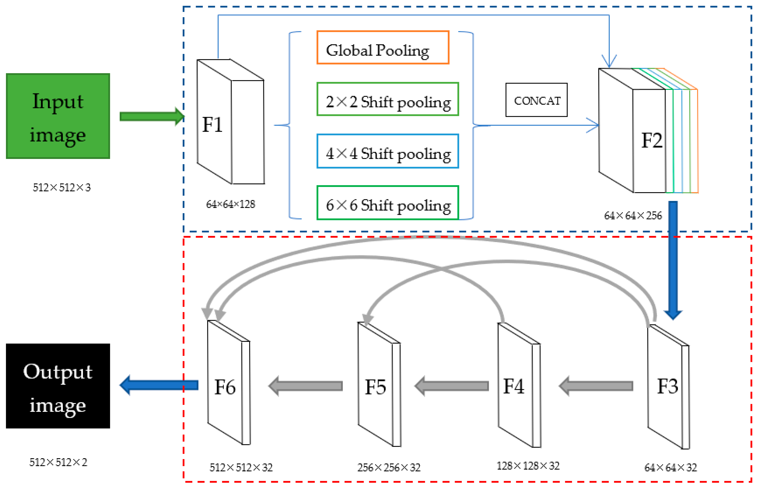
2.1. Architecture of Shift Pooling PSPNet

PSPNet is a deep learning network proposed by Zhao et al. in 2017. The core module is the pyramid pooling module, which can aggregate the contextual information of different scales so as to improve the ability to obtain multiscale features. The specific model structure is shown in Figure 1. Firstly, the classical neural networks, such as vgg16 and resnet101, are used to extract the features of the input image. This step is the content represented by the CNN box in Figure 1. Then, the obtained feature map is pooled at different scales to enhance the actual receptive field of each pixel, which is called the pyramid pooling module in this paper. The dotted rectangle in Figure 1 is the pyramid pooling module. The red part pools the whole feature map into one pixel, then convolution with a kernel of 1 × 1 reduces the depth to 1/4 of the original. The yellow module divides the whole feature map into 4 grids and pools them into 1 pixel, a feature map with the size of 2 × 2 pixel is obtained, and then, convolution with a kernel of 1 × 1 reduces the depth to 1/4 of the original. The blue module divides the whole feature map into 9 grids and pools them into 1 pixel, a feature map with the size of 3 × 3 pixel is obtained, and then, convolution with a kernel of 1 × 1 reduces the depth to 1/4 of the original. The green module divides the whole feature map into 36 grids and pools them into 1 pixel, a feature map with the size of 6 × 6 pixel is obtained, and then, convolution with a kernel of 1 × 1 reduces the depth to 1/4 of the original. Finally, the pooled results of four different scales are upsampled to the same size as the input feature map, concatenated with the input feature map, then fused by convolution to obtain the prediction results.

PSPNet can capture multi-scale local features by using the pyramid pooling module, but the pixels at the edge of the grid cannot cross the grid to capture the entire local features. The pixels at the corner of the grid can capture only 1/4 of the local features, which is obviously not enough. Moreover, the feature map output by the pyramid pooling module is directly upsampled to the size of the input image, so the ability to capture local details is weak. In order to address this problem, this paper proposes an improved PSPNet, the architecture of which is shown in Figure 2. Like PSPNet, in our method, the input image passes through one of classic backbones to obtain the feature map F1. In this model, resnet101 is used as the backbone, and the features extracted from the “block2/unit_4/bottleneck_v2/conv1” layer are used as the output feature map F1 of the backbone, so the size of feature map F1 is 64 × 64 × 128. Feature map F1 is sent into the shift pyramid pooling module instead of the pyramid pooling module in PSPNet, as shown in the blue dotted rectangle in Figure 2. Similar to PSPNet, the shift pyramid pooling module also performs multi-scale pooling, but for the top global pooling, similar to PSPNet, the following three scales of pooling are shift pooling instead of normal pooling, the details of which are introduced later. The depth of the feature map output by each shift pooling is 1/4 of the input feature map F1. Finally, the output features of the four scales are concatenated with the input feature map F1 to obtain feature map F2, the depth of which is twice that of the input feature map F1. Convolution with a kernel of 1 × 1 is followed to adjust the depth to 1/4 of the input feature map F1. After the whole shift pyramid pooling module, the size of the obtained feature map F3 is the same as that of the input feature map F1, except the depth is 1/4 that of feature map F1. In this model, the size of feature map F3 is 64 × 64 × 32.

In order to avoid the loss of detailed features caused by PSPNet directly upsampling the feature map, feature map F3, which is output by the shift pyramid pooling module, is upsampled step by step, and the feature fusion of multiple scales is enhanced by the dense connection, as shown in the red rectangle of Figure 2. Firstly, transpose convolution is used to upsample the feature map F3 twice, and then, convolution with a kernel of 3 × 3 follows to obtain feature map F4, and the size of feature map F4 is 128 × 128 × 32. Secondly, transpose convolution is used to upsample feature map F4 twice and upsample feature map F3 four times. The results are concatenated, and then, convolution with a kernel of 3 × 3 follows to obtain fused feature map F5, and the size of feature map F5 is 256 × 256 × 32. Thirdly, feature map F5 is upsampled twice, feature map F4 is upsampled four times, and feature map F3 is upsampled eight times. All results are concatenated, and then, convolution with a kernel of 3 × 3 follows to obtain fused feature map F6, and the size of feature map F6 is 512 × 512 × 32. Finally, convolution with a kernel of 1 × 1 is used for adjusting the depth to the number of classifications. In this model, buildings are the only objects extracted from the remote sensing images, so the final output result is 512 × 512 × 2.

Table 1. Comparison of the parameter numbers before and after using the shift pooling and step-by-step upsampling modules.

Methods	Params (M)
PSPNet	42.57
PSPNet + shift pooling	42.62
PSPNet + our decoder	42.64
PSPNet + shift pooling + our decoder (shift pooling PSPNet)	42.69

shows the comparison of the parameters between each module of our proposed method and the original PSPNet. It can be seen that the number of parameters of the original PSPNet is 42.57 million. After replacing the pyramid pooling module with the shift pyramid pooling module, the parameters only increase by 0.05 million, and the percentage is only 0.12%. By adding the proposed step-by-step upsampling module to the original PSPNet, the number of parameters increased by 0.07 million, and the percentage is only 0.16%. The shift pyramid pooling module and step-by-step upsampling module are used at the same time in our proposed shift pooling PSPNet. According to Table 1, the parameters increase by only 0.12 million, and the percentage of increase is 0.28%. It can be seen that, compared to the original PSPNet, the parameters of shift pooling PSPNet we proposed increase only slightly, so it will not have a significant impact on the speed during both the training and inference.

2.2. Shift Pooling

The pooling used in the pyramid pooling of PSPNet divides a feature map into several grids equally, then maximum pooling or average pooling is used in each grid, and the result is upsampled to the original feature map size. This method results in the problem that the pixels at the edge of the grid cannot capture the entire local features across the grid, and the pixels at the corner of the grid can capture only 1/4 of the local features, which is obviously insufficient. As shown in Figure 3a, 2 × 2 normal pooling is used in the pyramid pooling module of PSPNet, and the whole feature map is bisected vertically and horizontally to obtain 4 grids. Since the yellow pixels are located at the corner of the grid, they can only capture the local features in the range of 1/4, while the green and blue pixels can only capture the local features in the range of 1/2, because they are located at the edges of the grid.

In order to make up for the above shortcomings, we propose a pooling method called shift pooling. As shown in Figure 3b, the division line of the grid is shifted horizontally by 1/2 the grid size, and the places without pixels are padded with the method of symmetrical replication, which will not change the pooling results. The feature map is then divided into 3 grids equally in the horizontal direction and bisected in the vertical direction, and 2 × 3 grids are obtained. The pixels in each grid are pooled to a pixel using the maximum pooling method and then upsampled to the size before pooling. Then, the nonpixel part in the feature map before padding is cut off using the slicing method, and the feature map is restored to the same size before padding. The pseudocode of horizontal shift pooling is shown in Algorithm 1.

After horizontal shift pooling, the green pixels can capture all the local features, but the yellow and blue pixels cannot capture all the local feature information, so the vertical shift is also required. As shown in Figure 3c, the division line of the grids is shifted vertically by 1/2 the grid size, and the places without pixels are padded with the method of symmetrical replication. The feature map is then divided into 3 grids equally in the vertical direction and bisected in the horizontal direction, and 3 × 2 grids are obtained. The pixels in each grid are pooled to a pixel using the maximum pooling method and then upsampled to the size before pooling. Then, the nonpixel part in the feature map before padding is cut off using the slicing method, and the feature map is restored to the same size before padding. The pseudocode of vertical shift pooling is shown in Algorithm 2.

Algorithm 1: Horizontal shift pooling

Input: feature map, pool_factor, depth

Output: feature map

1: Divide the size of the feature map by pool_factor to obtain the pooling size and stride. (For example, If the pool_factor is 2, the pooling size is half of the feature map size, and the stride equals pooling size.)

2: Obtain the size of padding on the left and right of the feature map; the value is half of the pooling size.

3: Pad the feature map on the left and right symmetrically to obtain feature map 1. 4: Maxpool feature map 1 with size and stride obtained by step 1 to obtain feature map 2. 5: Feature map 2 is convoluted with a 1 × 1 kernel into a feature map 3 with the same width and height, but the channel is deep. 6: Through batch normalization and activation layers, feature map 4 is obtained. 7: Upsample feature map 4 to the size of feature map 1 to obtain feature map 5.

8: Crop off the left and right padding parts of feature map 5 to obtain feature map 6.

9: Return feature map 6.

After vertical shift pooling, the blue pixels can also capture all the local features, but the yellow pixels can only capture 3/4. For example, the yellow pixel with an orange border in Figure 3c cannot capture the local feature in the upper left corner after horizontal and vertical shift. Therefore, it is also necessary to shift in both the horizontal and vertical directions. As shown in Figure 3d, the division line of the grid is shifted by 1/2 the grid size in the horizontal and vertical directions at the same time, the places without pixels are padded with the method of symmetrical replication, the feature map is divided into 3 grids equally both in the horizontal and vertical directions, and 3 × 3 grids are obtained. The pixels in each grid are pooled to a pixel using the maximum pooling method and then upsampled to the size before pooling. Then, the nonpixel part in the feature map before padding is cut off using the slicing method, and the feature map is restored to the same size before padding. The pseudocode of horizontal and vertical shift pooling is shown in Algorithm 3.

Algorithm 2: Vertical shift pooling

Input: feature map, pool_factor, depth

Output: feature map

1: Divide the size of the feature map by pool_factor to obtain the pooling size and stride.

2: Obtain the size of padding on the top and bottom of the feature map; the value is half of the pooling size.

3: Pad the feature map on the top and bottom symmetrically to obtain feature map 1. 4: Maxpool feature map 1 with size and stride obtained by step 1 to obtain feature map 2. 5: Feature map 2 is convoluted with a 1 × 1 kernel into feature map 3 with same width and height, but the channel is deep. 6: Through batch normalization and activation layers, feature map 4 is obtained. 7: Upsample feature map 4 to the size of feature map 1 to obtain feature map 5.

8: Crop off top and bottom padding parts of feature map 5 to obtain feature map 6.

9: Return feature map 6.

Algorithm 3: Horizontal and vertical shift pooling

Input: feature map, pool_factor, depth

Output: feature map

1: Divide the size of the feature map by pool_factor to obtain the pooling size and stride.

2: Obtain the size of padding on the left, right, top, and bottom of the feature map; the value is half of the pooling size.

3: Pad the feature map on the left and right symmetrically, then pad the top and bottom symmetrically again to obtain feature map 1. 4: Maxpool feature map 1 with the size and stride obtained by step 1 to obtain feature map 2. 5: Feature map 2 is convoluted with a 1 × 1 kernel into a feature map 3 with same width and height, but the channel is deep. 6: Through batch normalization and activation layers, feature map 4 is obtained. 7: Upsample feature map 4 to the size of feature map 1 to obtain feature map 5.

8: Crop off the left, right, top, and bottom padding parts of feature map 5 to obtain feature map 6.

9: Return feature map 6.

After horizontal and vertical shift pooling, yellow pixels can also capture the complete local features. When the four pooling methods of normal pooling, horizontal shift pooling, vertical shift pooling, and horizontal and vertical shift pooling are combined, each pixel in the feature map can capture the entire local feature. As shown in Figure 3, a yellow pixel with an orange border can only capture 1/4 of the local feature in (a), while when (a)–(d) are used together, the pixel can actually capture the entire local feature, which is shown in the green rectangle of (e).

The detailed architecture of the shift pooling model in Figure 2 is shown in Figure 4. Firstly, feature map F1 with a size of 64 × 64 × 128 output by the backbone is pooled normally to obtain feature map F2, feature map F3 is obtained by horizontal shift pooling, feature map F4 is obtained by vertical shift pooling, and feature map F5 is obtained by horizontal and vertical shift pooling. F2–F5 all have the size 64 × 64 × 32. Then, F2–F5 are concatenated to obtain feature map F6 with a size of 64 × 64 × 128. Finally, a convolution with a kernel of 1 × 1 adjusts the depth of F6 to 32 to obtain feature map F7, and the size of feature map F7 is 64 × 64 × 32. After the shift pooling module, each pixel in the feature map can fully capture the whole local feature information.

3. Experiment and Results

3.1. WHU Building Dataset and Preprocessing

The aerial dataset of the WHU building open dataset [36] was chosen for our experiment. This dataset was labeled by Professor Ji Shunping. The aerial dataset consists of more than 220,000 independent buildings extracted from aerial images with 0.075-m spatial resolution and 450 km² covering Christchurch, New Zealand. The original aerial data are from the New Zealand land information service website, and the ground resolution is 0.075 m. In order to train on most computers, the data were downsampled to 0.3 m at the ground resolution and then cropped into 8189 tiles with 512 × 512 pixels. All tiles were divided into three parts: training set (including 130,500 buildings), validation set (including 14,500 buildings), and test set (including 42,000 buildings). The training dataset includes 4736 tiles, the validation dataset includes 1036 tiles, and the test dataset includes 2416 tiles. Each tile contains one three-channel TIF format image and one single-channel TIF format label.

In order to speed up reading the data from the hard disk during training, we wrote data compression software in Python to compress the training, verification, and test datasets into a TFrecord file. TFrecord is the official format of TensorFlow, using data stored in binary form.

Some scholars use data augmentation to solve the problem of limited training data [37]. However, few-shot learning is the development direction of deep learning algorithms [38]. Moreover, the number of tiles in the WHU building dataset is adequate, and the same training and test data are convenient for comparison among other scholars. Therefore, no dataset augmentation was used in this work.

3.2. Massachusetts Building Dataset and Preprocessing

The Massachusetts building dataset [39] consists of images of the Boston area of the United States, and the entire dataset covers about 340 square kilometers. The dataset has 151 aerial images in total, the size of each image is 1500 × 1500 pixels, the ground resolution is 1 m, the format is three-channel TIF, and the corresponding annotation image is single-channel TIF format data.

Due to the limitations of the computer hardware used in the experiment, we cropped the original image to 512 × 512 pixels, so nine images could be cropped out of one original image. Where there were no pixels in the original image, the pixel value was set to 0, and a total of 1359 images were obtained. We divided the dataset into a training set and a test set. There were 1233 images in the training set and 126 images in the test set. Like the WHU dataset, we used our own Python program to convert cropped images into the TFrecord format of TensorFlow to speed up the reading of data from the hard disk and save training time.

3.3. Hardware and Settings for Experiment

The CPU model used is an Intel i5-9400f with Kingston DDR4 8 G memory, and the GPU model is an NVIDIA GeForce RTX 2060 super 8 G. The environment in which the code was written and run is Python 3.6.8.

AdamOptimizer [40] was used for back propagation, and the learning rate was set to 0.0001 during training. The sum of L2 regularization and binary cross-entropy was used as the total loss to prevent overfitting. The total loss is shown in Formula (1). The maximum number of training epochs was set to 100. After each epoch, an evaluation was performed on the validation dataset. Unlike the stopping standard used in [21], in which training was stopped if the metrics in the validation set no longer increased for 10 consecutive epochs, our stopping standard was that, if the loss in the validation set no longer reduced for 10 consecutive epochs, then training was stopped. In this paper, the backbone of the original PSPNet and our shift pooling PSPNet are both resnet101.

$$\left.\begin{array}{c}\mathrm{TotalLoss}=\mathrm{BinaryCrossEntropy}+L2\\ L2=||w|{|}_2^2={\displaystyle \sum _i\left|w_i^2\right|}\end{array}\right\}$$

(1)

3.4. Evaluation Metrics

Some scholars use recall and precision as evaluation metrics, but the increase in one of these two metrics may lead to the decrease in the other, so, alone, they are not reliable. To this end, we used the more scientific F1-score for evaluation, together with the most commonly used mIoU and accuracy, a total of three evaluation metrics.

The formula for mIoU is:

$$\mathrm{mIoU}=\frac{1}{N+1}{\displaystyle \sum _{i=0}^N\frac{TP}{TP+FN+FP}}$$

(2)

The formula for accuracy is:

$$\mathrm{Accuracy}=\frac{TP+TN}{TP+TN+FP+FN}$$

(3)

The formula for the F1-score is:

$$\mathrm{F}1-\mathrm{Score}=\frac{2\times Precison\times Recall}{Precison+Recall}$$

(4)

where the precision and recall are:

$$Precison=\frac{TP}{TP+FP}$$

(5)

$$Recall=\frac{TP}{TP+FN}$$

(6)

In all formulas, N is the number of the foreground. TP is the abbreviation of true positives—that is, the number of pixels correctly predicted as the foreground. FP is the abbreviation of false positives—that is, the number of background pixels misjudged as the foreground. TN is the abbreviation of true negatives—that is, the number of pixels correctly predicted as the background. FN is the abbreviation of false negatives—that is, the number of foreground pixels misjudged as background. In Equation (2), the building and background are regarded as the foreground to obtain IoU, then the average value is taken as mIoU. The foreground in Equations (4)–(6) is the building.

3.5. Results on WHU Building Dataset

The comparison results of the main segmentation networks on the test dataset of the WHU building dataset are shown in

Table 2. Results of classic semantic segmentation on the WHU building test dataset.

Methods	mIoU	F1-Score	Accuracy
SETR	83.5	83.1	96.3
MSST-Net	88.0	88.2	97.4
SegNet	83.8	83.5	96.4
DeepLab V3	84.6	84.3	96.7
PSPNet	86.7	86.8	97.0
SPNet	87.3	87.5	97.2
BiSeNet V2	87.6	87.8	97.3
CFENet	88.1	88.2	97.5
Ours	89.1	89.4	97.7

. As shown in Table 2, our improved method based on PSPNet performs best in all evaluation metrics: mIoU, F1-score, and accuracy.

SegNet, DeepLabV3, SPNet, BiSeNetV2, CFENet, and PSPNet are classic semantic segmentation networks based on convolutional neural networks. Among them, in terms of evaluation metrics, the best is CFENet, followed by BiSeNetV2, SPNet, PSPNet, and DeepLabV3, and the worst is SegNet. Due to the use of the pyramid pooling module, PSPNet addresses the problem that the actual receptive field of the multilayer convolutional neural network is smaller than the theoretical receptive field. For mIoU, PSPNet is 2.1% higher than DeepLabV3; for the F1-score, PSPNet is 2.5% higher than DeepLabV3; and for accuracy, PSPNet is 0.3% higher than DeepLabV3. Compared with SegNet, mIoU of PSPNet is 2.9% higher than that of SegNet, the F1-score of PSPNet is 3.3% higher than that of SegNet, and the accuracy of PSPNet is 0.6% higher than that of SegNet. It can be seen that the PSPNet network itself is excellent. Due to the combined use of pyramid pooling and strip pooling, the effect of SPNet is the better than PSPNet. The mIoU of SPNet is 0.6% higher than PSPNet, the F1-score is 0.7% higher, and the accuracy is 0.2% higher. However, BiSeNetV2, which is the Bilateral Segmentation Network, performs a little better than SPNet. The performance of CFENet is even better than that of BiSeNetV2: the mIoU is as high as 88.1%, the F1-score is 88.2%, and the accuracy is 97.5%.

MSST-Net and SETR are networks based on Transformer. It can be seen that the performance of SETR is poor. Compared with the other networks, the three metrics are the worst. MSST-Net fuses the multi-scale feature of Swin Transformer, so all the metrics are greatly improved. Compared with SETR, the mIoU of MSST-Net increased by 4.5%, the F1-score of MSST-Net increased by 5.1%, and the accuracy of MSST-Net increased by 1.1%.

Our network improved from PSPNet is the best among all the network models, because it fixes the disadvantage that the pixels on the edge of the pooling grid cannot fully capture the entire local feature, so all the evaluation metrics are significantly improved. Compared with the original PSPNet network, our network improves the mIoU by 2.4%, F1-score by 2.6%, and accuracy by 0.7%. Even compared with MSST-Net, which is based on multi-scale Swin Transformer, the mIoU of our network increases by 1.1%, the F1-score increases by 1.2%, and the accuracy increases by 0.3%. This is enough to show that there is no meaningful difference in results between the convolutional neural network and Transformer. As long as an appropriate algorithm is designed, a convolutional neural network can also capture local and global features well, so as to achieve high-precision semantic segmentation.

Figure 5, Figure 6 and Figure 7 show the comparison results of various classical segmentation models with our method on large buildings, small buildings, and roads, which have a similar texture to buildings.

As can be seen in the red circle of Figure 5, the segmentation ability of DeepLabV3 with small buildings is very poor. In brief, small buildings cannot be predicted, as the edges and corners of the buildings are relatively smooth, with few right angles. Although other segmentation networks can also predict small buildings, such as the original PSPNet network, our method is the best one in the segmentation of small buildings. Our method uses the shift pyramid pooling module instead of the pyramid pooling module in PSPNet, which can enhance the ability of the network to capture local features at the edge of the pooling grid. Therefore, small buildings at the edge of the pooling grid can also be predicted well by our improved PSPNet. For example, the position of two small buildings in the red circle of Figure 5 is exactly close to edge of the grid of pooling with 2 × 2, and pixels at edges cannot cross the pooling grid to capture all local feature information, so the segmentation effect of the original PSPNet network is poor, but the segmentation effect of our method is significantly improved and even close to the label.

It can be seen from the prediction of the red circle in Figure 6 that there are holes in the large buildings predicted by the segmentation network models SETR and MSST-Net, which are based on Transformer, while there are no obvious holes in the large buildings predicted by the network models SegNet, DeepLabV3, PSPNet, SPNet, BiSeNetV2, CFENet, and our method, which are based on convolution. The segmentation network model SETR and MSST-Net, which are based on Transformer, have better predictions on the edges of large targets, especially the edges of buildings predicted by MSST-Net that are basically straight lines and right angle corners. There are some concaves on the edges of the large building predicted by SegNet and PSPNet, which is because the original PSPNet has an insufficient ability to capture entire local features, and our method can better capture local features due to the improvement in this aspect, so the edge of the prediction building is much better and almost the same as the label.

It can be seen from the red circle area in Figure 7 that, because some cement roads have a similar texture to the roofs of buildings, many segmentation networks misjudge the pixels of the road as pixels of a building. In particular, the misjudgment of PSPNet is the most obvious one among all the networks, and it is followed by SETR, DeepLabV3, and BiSeNetV2, while the misjudgment of SPNet is lower in this regard. MSST-Net fuses the multi-scale features of Swin Transformer, which allow it to better capture the local features of multiple scales, so it performs well in this regard, and there are very few misjudged pixels. Although SPNet and CFENet do not predict roads as buildings incorrectly, the edge distortions of houses with correct predictions are serious.

Our network is the best one among all the networks in this regard. Due to the improvement of the pyramid pooling module, each pixel in the feature map, including the pixels at the edges and corners of the pooling grid, can capture enough local feature information. With a more comprehensive analysis of local feature information, there are no pixels of road misjudged as building pixels by our network.

3.6. Results on Massachusetts Building Dataset

The comparison results of the classic segmentation networks for the Massachusetts building dataset are shown in

Table 3. Results of classic semantic segmentation on the Massachusetts building test dataset.

Methods	mIoU	F1-Score	Accuracy
SETR	67.9	63.5	90.2
MSST-Net	71.0	68.6	90.9
SegNet	69.9	66.7	90.7
DeepLab V3	67.5	63.8	89.3
PSPNet	71.8	70.0	90.8
SPNet	70.6	68.0	90.6
BiSeNet V2	72.2	70.3	91.2
CFENet	71.4	68.7	91.4
Ours	75.4	74.3	92.6

. Our method based on shift pooling performs best in all evaluation metrics: mIoU, F1-score, and accuracy.

SegNet, DeepLabV3, SPNet, BiSeNetV2, CFENet, and PSPNet are classic semantic segmentation networks based on the convolutional neural network. Among them, in terms of evaluation metrics, the best is BiSeNetV2, PSPNet is the second best, the worst is DeepLabV3, SegNet is the second worst, CFENet and SPNet are in the middle.

MSST-Net and SETR are networks based on Transformer. MSST-Net achieved a better performance than SETR, but on the whole, their performances were not as good as the convolutional neural network. Unlike the MSST-Net performance being better than BiSeNetV2 and PSPNet on the WHU building dataset, BiSeNetV2 and PSPNet performance was better than MSST-Net on the Massachusetts building dataset. This is because the annotation accuracy of the Massachusetts building dataset is relatively low, and there is too much noise. When using supervised learning, the advantages of the MSST-Net that performs well on the WHU building dataset are suppressed due to the influence of incorrectly labeled pixels. This also shows that BiSeNetV2 and PSPNet have better anti-noise ability than MSST-Net.

Our network is the best among all the network models whether a CNN or Transformer is used, because it improves on PSPNet, and it fixes the disadvantage of PSPNet that the pixels on the edges of the pooling grid cannot fully capture the entire local feature, so all the evaluation metrics are significantly improved. Compared with the original PSPNet network, our network improves the mIoU by 3.6%, F1-score by 4.3%, and accuracy by 1.8%. Compared with the second best network among all network models, our network improves the mIoU by 3.2%, F1-score by 4.0%, and accuracy by 1.4%. It can be seen that the shift pooling structure has a stronger anti-noise ability for the dataset with low annotation accuracy.

Figure 8 shows the segmentation results of small buildings in various segmentation networks on the Massachusetts building dataset. It can be seen that DeepLabV3 and PSPNet perform poorly in small building segmentation, as many small buildings are not detected, and there is an obvious error that several small buildings close to each other are predicted as a continuous building, as shown in the red rectangle in Figure 8. SegNet, SPNet, BiSeNetV2, and CFENet, which are also based on convolutional neural networks, perform better than DeepLabV3 and PSPNet; they hardly predict two small buildings close to each other as one continuous building. However, the shapes of larger buildings are slightly worse than DeepLabV3 and PSPNet, as shown in the red circle in Figure 8.

The performance of the networks, SETR and MSST-Net, which are based on Transformer, on the segmentation of small buildings is better than that of DeepLabV3 and PSPNet. The boundaries of the predicted small buildings are very clear, as there is no error where two or more small buildings close to each other are predicted as one building. The boundaries of the larger buildings segmented by MSST-Net are closer to the straight line, which is consistent with the label. However, the segmentation of larger buildings by SETR is the worst among all the networks, and a large building is wrongly segmented as multiple small buildings, as shown in the red circle in Figure 8.

In general, our network achieves good performance in segmentation for small buildings, with clear boundaries and few missed inspections; there is no case where multiple adjacent small buildings are segmented as a larger building. Meanwhile, the larger buildings boundaries predicted by our network are closest to the label among all the network models.

4. Discussion

4.1. Ablation Experiment

In order to prove that the shift pooling module and the step-by-step upsampling module proposed by us can improve the effect of PSPNet extracting houses from remote sensing images, we conducted ablation experiments on the Massachusetts building dataset, and the results are shown in

Table 4. Comparison before and after using shift pooling and step-by-step. upsampling modules on the Massachusetts building test dataset.

Methods	mIoU	F1-Score	Accuracy
PSPNet	71.8	70.0	90.8
PSPNet + Our decoder	72.8	71.1	91.4
PSPNet + shift pooling	73.8	72.6	91.7
PSPNet + Our decoder + shift pooling (shift pooling PSPNet)	75.4	74.3	92.6

.

It can be seen from Table 4 that mIoU increased by 1.0% when only using the step-by-step upsampling module. The mIoU increased by 2.0% when only using shift pooling instead of normal pooling. The mIoU increased by 3.6% when these two modules were used at the same time. Therefore, these two modules both can make shift pooling PSPNet much better than the original PSPNet model.

As we said in the introduction, PSPNet can use many networks as backbones, including some excellent networks in the future. To verify that our shift pooling PSPNet is better than the original PSPNet when various networks are used as the backbone, we used three different networks, resNet50, resNet101, and resNet152, as backbones for comparative experiments. The results are shown in

Table 5. Comparison of different backbones on the Massachusetts building test dataset.

Methods	Backbone	mIoU	F1-Score	Accuracy
PSPNet	ResNet50	72.1	70.2	91.2
Shift pooling PSPNet		75.3	74.4	92.4
PSPNet	ResNet101	71.8	70.0	90.8
Shift pooling PSPNet		75.4	74.3	92.6
PSPNet	ResNet152	71.9	69.9	91.1
Shift pooling PSPNet		75.7	74.8	92.5

.

The experimental results show that our shift pooling PSPNet performs better than the original PSPNet on all backbones. When ResNet152 is used as the backbone, the mIoU increases by 3.6%.

4.2. Feature Visualization

In order to visualize the feature map captured by the shift pooling pyramid module and pyramid pooling module, we selected an image in the WHU building dataset for visualization, and the results are shown in Figure 9. In Figure 9a is a color image, (b) is the corresponding feature visualization of the pyramid pooling module in PSPNet, and (c) is the corresponding feature visualization of the shift pyramid pooling module in shift pooling PSPNet.

The visualization feature map is the output of convolution with a 3 × 3 kernel after the concatenated feature map of four-scale shift pooling; there are 32 channels in total, so we add them together. Since the value of the visualization feature map is not necessarily between 0 and 255, in order to display it as an image, we mapped each pixel between 0 and 255, as shown in Equation (7).

$$P_{\mathrm{visualization}}=\frac{P_{\mathrm{feature}}-P_{\min }}{P_{\max }-P_{\min }}$$

(7)

where $P_{\mathrm{visualization}}$ represents the pixel value for display, $P_{\mathrm{feature}}$ represents the pixel value of the feature map, and $P_{\max }$ and $P_{\min }$ represent the maximum and minimum values of the feature map, respectively.

It can be seen from the visualization results of the feature map that the shift pyramid pooling module is much better for the feature extraction of a building, and the building edges are very clear, while the differences between the building and background in the feature map of the pyramid pooling module is not obvious, and the building edges are very fuzzy, which cannot effectively distinguish between the building and background.

4.3. Generalizations Discussion

In order to discuss the generalization of the model, we list the mIoU values of all the models in the validation dataset and test the dataset of the WHU building dataset in

Table 6. mIoU of all networks on the validation and test datasets of the WHU building dataset.

Methods	mIoU of Validation Dataset	mIoU of Test Dataset	Test Validation
SETR	82.8	83.5	0.7
MSST-Net	88.1	88.0	-0.1
SegNet	86.3	83.8	-2.5
DeepLab V3	85.2	84.6	-0.6
PSPNet	87.4	86.7	-0.7
SPNet	87.9	87.3	-0.6
BiSeNet V2	87.4	87.6	0.2
CFENet	89.0	88.1	-0.9
Ours	89.6	89.1	-0.5

. It can be seen that the generalization of networks based on Transformer is good. Although the performance of SETR on both the validation dataset and the test dataset is poor, the generalization of SETR is the best, and the mIoU on the test dataset is 0.7% higher than that on the validation dataset. The generalization of MSST-Net is also good, and the mIoU on the test dataset is only 0.1% lower than that on the validation dataset.

Among networks based on convolution, BiSeNet V2 has the best generalization, the mIoU on the test dataset is 0.2% higher than that on the validation dataset. Our shift pooling PSPNet is the second best, and the mIoU on the test dataset is only 0.5% lower than that in the validation dataset.

SegNet is the worst among all the networks, whether convolution-based or Transformer-based, and the mIoU on the test dataset is 2.5% lower than that in the validation dataset.

5. Conclusions

In this paper, we propose a pooling method called shift pooling and improve PSPNet on this basis. By shifting the position of the pooling grid, the pixels at the edge and corner of the pooling grid can capture the complete local feature information, so the results of the segmentation are improved.

We used SETR, SegNet, DeepLabV3, PSPNet, SPNet, MSST-Net, and our proposed network to compare using the open dataset. The results showed that our method performs best in three evaluation metrics of the mIoU, F1-score, and accuracy. From the prediction results, our method can accurately predict small buildings, the shapes of which are very close to the label. From the prediction results of large buildings, there are no holes in the buildings predicted by our segmentation network, the edges of the buildings are close to straight lines, and the corners of the buildings are right angles. In the road prediction results, our segmentation network does not misjudge the road pixels, the texture of which is similar to that of the buildings.

In future work, we will continue to explore how to apply the shift pooling method to other segmentation networks, so as to design a better semantic segmentation network model.

References

1. Gislason, P.O.; Benediktsson, J.A.; Sveinsson, J.R. Random Forest Classification of Multisource Remote Sensing and Geographic Data. In Proceedings of the IGARSS 2004, 2004 IEEE International Geoscience and Remote Sensing Symposium, Anchorage, AK, USA, 20–24 September 2004; Volume 2, pp. 1049–1052. [Google Scholar] [CrossRef]
2. Oommen, T.; Baise, L.G. A New Approach to Liquefaction Potential Mapping using Satellite Remote Sensing and Support Vector Machine Algorithm. In Proceedings of the IGARSS 2008–2008 IEEE International Geoscience and Remote Sensing Symposium, Boston, MA, USA, 6–11 July 2008; pp. III-51–III-54. [Google Scholar] [CrossRef]
3. Shen, W.; Wu, G.; Sun, Z.; Xiong, W.; Fu, Z.; Xiao, R. Study on classification methods of remote sensing image based on decision tree technology. In Proceedings of the 2011 International Conference on Computer Science and Service System (CSSS), Nanjing, China, 27–29 June 2011; pp. 4058–4061. [Google Scholar] [CrossRef]
4. Zhou, Y.; Chen, H.; Zhu, Q. The research of classification algorithm based on fuzzy clustering and neural network. In Proceedings of the IEEE International Geoscience and Remote Sensing Symposium, Toronto, ON, Canada, 24–28 June 2002; Volume 4, pp. 2525–2527. [Google Scholar] [CrossRef]
5. Lecun, Y.; Bottou, L.; Bengio, Y.; Haffner, P. Gradient-based learning applied to document recognition. Proc. IEEE 1998, 86, 2278–2324. [Google Scholar] [CrossRef]
6. Simonyan, K.; Zisserman, A. Very deep convolutional networks for large-scale image recognition. In Proceedings of the International Conference on Learning Representations, San Diego, CA, USA, 7–9 May 2015; pp. 1–14. Available online: https://arxiv.org/abs/1409.1556 (accessed on 3 July 2021).
7. Long, J.; Shelhamer, E.; Darrell, T. Fully convolutional networks for semantic segmentation. In Proceedings of the IEEE Conference on Computer Vision and Pattern Recognition, Washington, DC, USA, 7–12 June 2015; pp. 3431–3440. [Google Scholar]
8. Ronneberger, O.; Fischer, P.; Brox, T. Convolutional networks for biomedical image segmentation. In Proceedings of the 2015 Medical Image Computing and Computer Assisted Intervention, Piscataway, NJ, USA, 5–9 October 2015; pp. 234–241. [Google Scholar]
9. Badrinarayanan, V.; Kendall, A.; Cipolla, R. Segnet: A deep convolutional encoder-decoder architecture for image segmentation. IEEE Trans. Pattern Anal. Mach. Intell. 2017, 39, 2481–2495. [Google Scholar] [CrossRef] [PubMed]
10. Zhao, H.; Shi, J.; Qi, X.; Wang, X.; Jia, J. Pyramid scene parsing network. In Proceedings of the 2017 IEEE Conference on Computer Vision and Pattern Recognition (CVPR), Honolulu, HI, USA, 21–26 July 2017; pp. 6230–6239. [Google Scholar]
11. Chen, L.C.; Papandreou, G.; Kokkinos, I.; Murphy, K.; Yuille, A.L. Semantic image segmentation with deep convolutional nets and fully connected crfs. Comput. Sci. 2014, 357–361. Available online: https://arxiv.org/abs/1412.7062 (accessed on 13 July 2021).
12. Chen, L.; Papandreou, G.; Kokkinos, I.; Murphy, K.; Yuille, A.L. DeepLab: Semantic image segmentation with deep convolutional nets, atrous convolution, and fully connected crfs. IEEE Trans. Pattern Anal. Mach. Intell. 2018, 40, 834–848. [Google Scholar] [CrossRef] [PubMed]
13. Rethinking Atrous Convolution for Semantic Image Segmentation. 2017. Available online: https://arxiv.org/abs/1706.05587 (accessed on 13 July 2021).
14. Liu, P.; Liu, X.; Liu, M.; Shi, Q.; Yang, J.; Xu, X.; Zhang, Y. Building footprint extraction from high-resolution images via spatial residual inception convolutional neural network. Remote Sens. 2019, 11, 830. [Google Scholar] [CrossRef]
15. Liu, Y.; Zhou, J.; Qi, W.; Li, X.; Gross, L.; Shao, Q.; Zhao, Z.; Ni, L.; Fan, X.; Li, Z. ARC-Net: An Efficient Network for Building Extraction From High-Resolution Aerial Images. IEEE Access 2020, 8, 154997–155010. [Google Scholar] [CrossRef]
16. Yi, Y.; Zhang, Z.; Zhang, W.; Zhang, C.; Li, W.; Zhao, T. Semantic Segmentation of Urban Buildings from VHR Remote Sensing Imagery Using a Deep Convolutional Neural Network. Remote Sens. 2019, 11, 1774. [Google Scholar] [CrossRef] [Green Version]
17. Diakogiannis, F.I.; Waldner, F.; Caccetta, P.; Wu, C. Resunet-a: A deep learning framework for semantic segmentation of remotely sensed data. ISPRS J. Photogramm. Remote Sens. 2020, 162, 94–114. [Google Scholar] [CrossRef]
18. Ye, Z.; Fu, Y.; Gan, M.; Deng, J.; Comber, A.; Wang, K. Building extraction from very high resolution aerial imagery using joint attention deep neural network. Remote Sens. 2019, 11, 2970. [Google Scholar] [CrossRef]
19. Yu, B.; Yang, L.; Chen, F. Semantic segmentation for high spatial resolution remote sensing images based on convolution neural network and pyramid pooling module. IEEE J. Sel. Top. Appl. Earth Obs. Remote Sens. 2018, 11, 3252–3261. [Google Scholar] [CrossRef]
20. Zheng, S.; Lu, J.; Zhao, H.; Zhu, X.; Luo, Z.; Wang, Y.; Fu, Y.; Feng, J.; Xiang, T.; Torr, P.H.S.; et al. Rethinking Semantic Segmentation from a Sequence-to-Sequence Perspective with Transformers. In Proceedings of the IEEE/CVF Conference on Computer Vision and Pattern Recognition, Seattle, WA, USA, 13–19 June 2020. [Google Scholar]
21. Yuan, W.; Xu, W. MSST-Net: A Multi-Scale Adaptive Network for Building Extraction from Remote Sensing Images Based on Swin Transformer. Remote Sens. 2021, 13, 4743. [Google Scholar] [CrossRef]
22. Liu, Z.; Lin, Y.; Cao, Y.; Hu, H.; Wei, Y.; Zhang, Z.; Lin, S.; Guo, B. Swin Transformer: Hierarchical Vision Transformer using Shifted Windows. In Proceedings of the IEEE/CVF International Conference on Computer Vision, Montreal, QC, Canada, 10–17 October 2021. [Google Scholar]
23. Pan, X.; Yang, F.; Gao, L.; Chen, Z.; Zhang, B.; Fan, H.; Ren, J. Building extraction from high-resolution aerial imagery using a generative adversarial network with spatial and channel attention mechanisms. Remote Sens. 2019, 11, 917. [Google Scholar] [CrossRef]
24. Protopapadakis, E.; Doulamis, A.; Doulamis, N.; Maltezos, E. Stacked autoencoders driven by semi-supervised learning for building extraction from near infrared remote sensing imagery. Remote Sens. 2021, 13, 371. [Google Scholar] [CrossRef]
25. Wang, Y.; Zhao, L.; Liu, L.; Hu, H.; Tao, W. URNet: A U-Shaped Residual Network for Lightweight Image Super-Resolution. Remote Sens. 2021, 13, 3848. [Google Scholar] [CrossRef]
26. Liu, H.; Cao, F.; Wen, C.; Zhang, Q. Lightweight multi-scale residual networks with attention for image super-resolution. Knowl.-Based Syst. 2020, 203, 106103. [Google Scholar] [CrossRef]
27. Cheng, D.; Liao, R.; Fidler, S.; Urtasun, R. Darnet: Deep active ray network for building segmentation. In Proceedings of the IEEE/CVF Conference on Computer Vision and Pattern Recognition, Long Beach, CA, USA, 15–20 June 2019; pp. 7431–7439. [Google Scholar]
28. Yuan, W.; Xu, W. NeighborLoss: A Loss Function Considering Spatial Correlation for Semantic Segmentation of Remote Sensing Image. IEEE Access 2021, 9, 75641–75649. [Google Scholar] [CrossRef]
29. Chen, M.; Wu, J.; Liu, L.; Zhao, W.; Tian, F.; Shen, Q.; Zhao, B.; Du, R. DR-Net: An Improved Network for Building Extraction from High Resolution Remote Sensing Image. Remote Sens. 2021, 13, 294. [Google Scholar] [CrossRef]
30. Miao, Y.; Jiang, S.; Xu, Y.; Wang, D. Feature Residual Analysis Network for Building Extraction from Remote Sensing Images. Appl. Sci. 2022, 12, 5095. [Google Scholar] [CrossRef]
31. Hou, Q.; Zhang, L.; Cheng, M.-M.; Feng, J. Strip Pooling: Rethinking Spatial Pooling for Scene Parsing. In Proceedings of the IEEE/CVF Conference on Computer Vision and Pattern Recognition, Seattle, WA, USA, 30 March 2020. [Google Scholar]
32. Yu, C.; Gao, C.; Wang, J.; Yu, G.; Shen, C.; Sang, N. BiSeNet V2: Bilateral Network with Guided Aggregation for Real-Time Semantic Segmentation. Int. J. Comput. Vis. 2021, 129, 3051–3068. [Google Scholar] [CrossRef]
33. Chen, J.; Zhang, D.; Wu, Y.; Chen, Y.; Yan, X. A Context Feature Enhancement Network for Building Extraction from High-Resolution Remote Sensing Imagery. Remote Sens. 2022, 14, 2276. [Google Scholar] [CrossRef]
34. ZWang, Z.; Du, B.; Guo, Y. Domain Adaptation With Neural Embedding Matching. IEEE Trans. Neural Netw. Learn. Syst. 2020, 31, 2387–2397. [Google Scholar] [CrossRef]
35. Na, Y.; Kim, J.H.; Lee, K.; Park, J.; Hwang, J.Y.; Choi, J.P. Domain Adaptive Transfer Attack (DATA)-based Segmentation Networks for Building Extraction from Aerial Images. IEEE Trans. Geosci. Remote Sens. 2020, 59, 5171–5182. [Google Scholar] [CrossRef]
36. Ji, S.P.; Wei, S.Q. Building extraction via convolutional neural networks from an open remote sensing building dataset. Acta Geod. Cartogr. Sin. 2019, 48, 448–459. [Google Scholar]
37. Lashgari, E.; Liang, D.; Maoz, U. Data augmentation for deep-learning-based electroencephalography. J. Neurosci. Methods 2020, 346, 108885. [Google Scholar] [CrossRef]
38. Liu, W.; Zhang, C.; Lin, G.; Liu, F. CRNet: Cross-reference networks for few-shot segmentation. In Proceedings of the 2020 IEEE/CVF Conference on Computer Vision and Pattern Recognition (CVPR), Seattle, WA, USA, 13–19 June 2020; pp. 4164–4172. [Google Scholar]
39. Mnih, V. Machine Learning for Aerial Image Labeling. Ph.D. Thesis, University of Toronto, Toronto, ON, Canada, 2013. [Google Scholar]
40. Kingma, D.P.; Ba, J. Adam: A method for stochastic optimization. In Proceedings of the 3rd International Conference for Learning Representations, San Diego, CA, USA, 7–9 May 2015; pp. 1–15. [Google Scholar]
Figure 1. Architecture of the PSPNet network model [10].
Remotesensing 14 04889 g001
Figure 2. Architecture of the shift pooling PSPNet network model. The green arrow is the backbone. The numbers under the input image, output image, and feature map are their size. The blue arrow is convolution with a kernel of 1 × 1, and the cyan arrow is transpose convolution. The area contained in the blue dashed rectangle is the encoding block, and the area contained in the red dashed rectangle is the decoding block.
Remotesensing 14 04889 g002
Figure 3. Shift pooling method. The size of the feature map is 16 × 16, the thin black line is the pixel border, and the thick black line is the pooling grid border. (a) Normal pooling, (b) horizontal shift pooling, (c) vertical shift pooling, and (d) pooling method of both horizontal and vertical shifts at the same time. (e) Receptive field of the yellow pixel with orange border after the four pooling methods of (a)–(d) are carried out at the same time.
Remotesensing 14 04889 g003
Figure 4. Shift pooling architecture.
Remotesensing 14 04889 g004
Figure 5. Prediction of classic networks for small buildings.
Remotesensing 14 04889 g005
Figure 6. Predictions of classic networks for large buildings.
Remotesensing 14 04889 g006
Figure 7. Road prediction results for building textures.
Remotesensing 14 04889 g007
Figure 8. Small building prediction results.
Remotesensing 14 04889 g008
Figure 9. Feature visualization of the pyramid pooling module and shift pooling pyramid. (a) One of the color images of the WHU building dataset. (b) Corresponding feature visualization of the pyramid pooling module in PSPNet. (c) Corresponding feature visualization of the shift pyramid pooling module in shift pooling PSPNet.
Remotesensing 14 04889 g009