1. Introduction
Today, financial markets are the object of increased interest from scientists, since the growth of the national economy and the well-being of individuals depend on their stability and effective functioning. Followers of the efficient-market hypothesis (EMH) [
1] prefer the “buy and hold” trading strategy, counting on the long-term growth of the selected asset. Within this theory, it is believed that it is impossible to beat stock indexes for a long time. However, a number of fundamental investors, e.g., Warren Buffet, who invest in accordance with the company’s current financial performance [
2], demonstrate their advantage over the dynamics of the stock index. In contrast to passive investment, active investment involves the purchase and sale of a security according to some condition that develops in the fundamental indicators of the company (fundamental analysis), or according to the current dynamics of quotations (technical analysis).
Fundamental analysis (FA) uses available news and other information to evaluate the direction of price movement in accordance with general economic, political and other considerations [
3]. Results of expert FA are regularly published on the websites of brokers and traders in the form of analytical reports and forecasts.
Technical analysis (TA) is associated with a formalized study of the dynamics of quotations and uses the entire arsenal of modern computer mathematics [
4]. In practice, traders usually use a combination of both types of analysis.
Thus, at the moment there is no algorithmic approach to making a trading decision that would have a clear advantage over others. Under these conditions, stock analysts prefer to justify their recommendations using channel strategies that are identified on simple calculating rules, insider information, market psychology, and visual interpretation [
5].
Various strategies of this type are described in well-known monographs on the management of market assets in investing and trading [
5,
6,
7,
8,
9,
10]. The main idea of channel strategies is to detect local trends in the development of the observed process. Such trends are assessed based on the localization of the current value of the asset in a certain range of its changes (i.e., a “channel”). Most often, channels are understood as areas of price changes of a priori selected width, parallel to the smoothed quotation average.
The simplicity and visual expressiveness of such strategies makes them extremely attractive, but their effectiveness, in general, is quite low. The main reason for this fact is the chaotic nature of the change in the values of quotations, described, for example, in [
11,
12]. The presence of dynamic chaos in the series of observations violates the basis of the entire probabilistic-statistical paradigm, i.e., the repeatability of experiments under identical conditions. In essence, the price series are formed by a flow of bifurcation points, for which arbitrarily small perturbations lead to an unpredictable development of the dynamics of the process.
It is difficult to assess the last statement analytically due to the fact that the right-hand sides of the corresponding systems of differential equations are random functions with constantly changing structures. Observations of financial markets demonstrate this: a newly found trend is very likely to reverse in the next moment. Therefore, back-test effective strategies could be effective later on by pure chance. The inability of trends to go on can be explained by the composition of the trading participants being an equilibrium balance. Trend-following traders (momentum traders) impact is compensated by market makers and mean reversion traders [
13]. At the same time, according to the inaction inertia theory [
14], individual investors who missed the opportunity to buy in at a good price withhold from a trade at a less favorable price, thus halting trend development. However, all of this becomes irrelevant when the fundamental valuation of the asset changes. If the majority of traders shares this opinion, a continuous trend may arise [
15,
16].
The only available approaches to effectiveness analysis of channel strategies and to investigating the chaotic nature of the observation series of market assets are numerical and statistical big data methods. In the work [
5], a large-scale empirical study of the effectiveness of the channel strategy developed by the authors was carried out from 31 July 1990 to 31 July 2010 for more than 3000 stocks of the NYSE and NASDAQ markets. It was shown that using the support and resistance levels (SAR), it is in general impossible to build a steadily profitable trading management system. However, making a decision on the price rollback from the support level works better than at the resistance level. The authors substantiate this fact by the globally growing trend in the stock market during this period.
This paper discusses performance of channel strategies, as well as their enhancement within nonstationary immersion environments, such as the currency market. We show that there are time intervals at which the use of this strategy will be profitable. The issue of the influence of optimization of the parameters of the trading system on its profitability is also considered.
We consider the EURUSD currency pair because it is the most liquid asset at the international financial market. This makes it possible to assess the effectiveness of channel strategies without the influence of such manipulative factors as insider trading or mistakes made by large investors.
2. Methods
As a basic model of market asset quotations, we will use the following additive model (Wald) [
10]:
where x
k, k = 1,…,n is a system component formed by sequentially smoothing the time series of initial observations y
k, k = 1,…,n and used in the process of making management decisions, and v
k, k = 1,…,n is the noise.
The traditional observation model for statistical analysis is based on the assumption that the system component is an unknown deterministic process, and the noise component is a stationary random process with independent increments. In the more general approach, based on the Bayesian concept [
17,
18,
19], the system component is also considered as a random process, and various computational schemes for sequential estimation of the conditional mean are used to identify it. As an example of the Bayesian approach, we can cite the Kalman filtration model [
20], in which the system component is modeled by a linearized model of the form x
k+1 = Φ
k+1/kx
k + w
k, k = 1,…,n, where w
k is the noise process that imitates the admissible errors in the system.
These traditional models allow us to construct classes of management strategies based on trend analysis [
7,
8,
9], each of which is effective only in a narrow range of possible variations of the observed process. The underlying reason for the low efficiency of the proposed trend indicators stems from the fundamental discrepancy between the traditional statistical approach and the nature of real observations. The following facts represented in Model (1) are the fundamental differences of the considered market asset observation series:
Their system component x
k, k = 1,…,n is an oscillatory nonperiodic process with a large number of local trends. This description indicates the possibility of interpreting this process as an implementation of the dynamic chaos model [
21,
22,
23,
24,
25,
26,
27,
28,
29]. However, the proof of this statement requires a strict formalization of the discrimination of deterministic chaotic and non-stationary random processes, which will require additional research.
The noise v
k, k = 1,…,n is a nonstationary random process roughly described by the Gaussian model with fluctuating parameters [
11,
12]. At the same time, noise deviations contain local trends, and their correlations and spectral characteristics change significantly over time [
30].
These characteristics violate the conditions of applicability of traditional statistical methods for effective decision making. Moreover, violation of the condition of repeatability prohibits any analytical assessments of forecasts and corresponding proactive management strategies. In essence, the main method of analyzing the quality of asset management in this case is numerical studies that assess the effectiveness of management algorithms over long observation intervals.
We have a number of financial instrument quote observations described by Model (1). Consider the simplest version of a single-channel management strategy. We define a “channel” as a range of observations limited by a range Yk = xk ± B, k = 1,…,n. Variations of observations inside the channel |yk − xk| = |δyk| ≤ B are interpreted as fluctuations that do not contain a pronounced trend, and the process itself is sometimes called a sideways trend or a flat. The choice of the channel width can be driven by various considerations. It usually lies in the range (1–3)sy, where sy is the estimate of the standard deviation (SD) δyk, k = 1,…,n. In general, the choice of channel width is an option that depends on the features of the TP management. In some cases, it can be a variable value Bk = Bk(yk), k = 1,…,n.
The current value of observations yk, k = 1,…,n breaking out of the channel is interpreted as the emergence of a trend in some management strategies. In the case of “playing by the trend”, this invokes a recommendation to open a position in the direction corresponding to the sign of the channel boundary. The position can be closed when a given level of gain (TP, “take profit”) or loss (SL, “stop loss”) is reached, or in accordance with other, more flexible rules defined by the management strategy.
The task of a trader or a trading robot is to choose a management strategy S and form a sequence of actions u
j, j = 1, …, M corresponding to it that provide maximum profit:
At the same time, each management strategy determines the moments of opening and closing a position (k
open,k
close)
j, j = 1,…,M, and, in some cases, the lot size. If the resulting amount at some k-th step turns out to be less than the trader’s available deposit R
0, then this means a complete loss. In order to isolate the system component, any technique of sequential filtration can be applied. In the simplest case, an exponential filter is used for this purpose, defined as [
31]:
with a smoothing coefficient α, whose value most often lies in the range [0.01,0.3].
The given simplified channel strategy makes it possible to remove many minor details. This makes the problem clear for the terminal task of producing the best proactive management for the selected class of management strategies.
2.1. Channel Strategy Based on Moving by the Trend
Let yk, k = 1,…,n be the observed monitoring process of an asset quotation with a given duration n. The system component xk, k = 1,…,n consists of an exponential filter (3) with a given smoothing coefficient α. The channel width is denoted as B, measured in pipses. Similarly, the levels of profit TP and the level of acceptable loss SL are set. The values of α, B, TP and SL are optional parameters. The choice of these parameters depends on the knowledge and intuition of the trader, as they completely determine the effectiveness of management. However, in trading, intuition and other human abilities often turn out to be ineffective. Thus, a need for strictly formalized and mathematically sound solutions arises.
The management strategy based on moving by the trend, which we have named CSF (channel strategy forward), consists in opening a position up or down when the process exits, respectively, the upper or lower boundary of the channel. The management algorithm consists of two rules: Open Up position at yk > xk + B or Open Dn at yk < xk − B, k = 1,…,n.
Note that a stricter formalization of this rule has the form yk-1 ≤ (xk-1 + B) & (yk > xk + B) or yk-1 ≥ (xk-1 + B) & (yk < xk + B), k = 1,…,n. Otherwise, a position will be opened at each step outside the channel. The position is closed either when the yk = yclose > yopen + TP or yk = yclose < yopen − SL levels are reached (with Open Up) or yclose < yopen − TP or yclose > yopen + SL (with Open Dn).
The considered version of the channel strategy is basic and can be easily augmented in various ways, presented, for example, in [
5,
6,
7,
8,
9]. In particular, it is natural to close a position at the moment of trend reversal, when the sign of the difference x
k − x
k −
nW, k = 1,…,n, nW being the size of the sliding observation window, changes to the opposite. However, this article is focused on the analysis of the fundamental features of channel management strategies, and, as a result, omits various complications.
2.2. Channel Strategy Based on Moving against the Trend
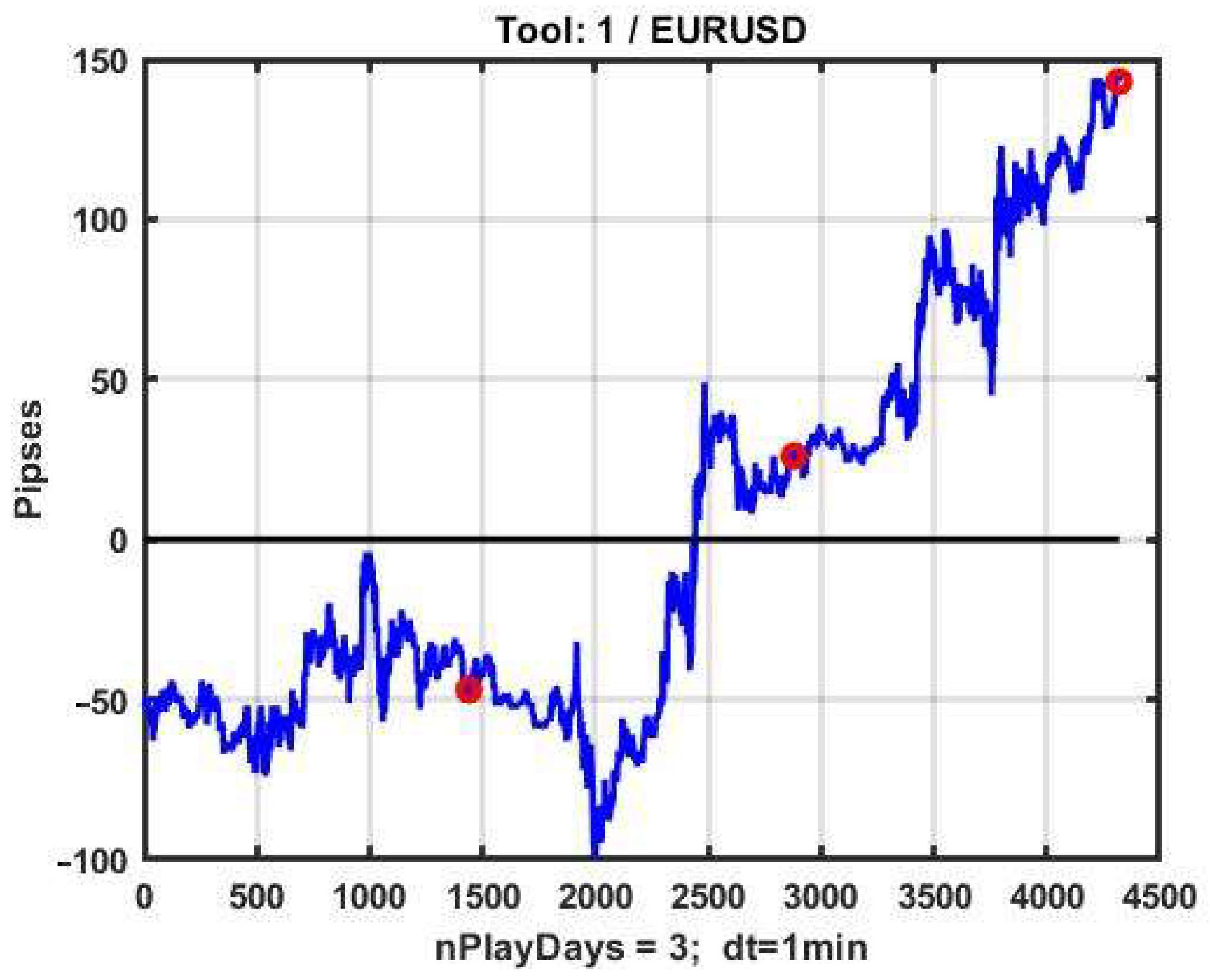
We will now consider an alternative interpretation of the observed process exiting the channel boundaries as another well-known channel strategy. In this case, the exit of the quotation from the channel is considered as a random deviation of the asset value, which inevitably triggers market compensation mechanisms that return the process to the limits of normalized fluctuations, i.e., to the limits of the channel. We will call this approach a channel strategy of playing against the trend (CSB, channel strategy back).
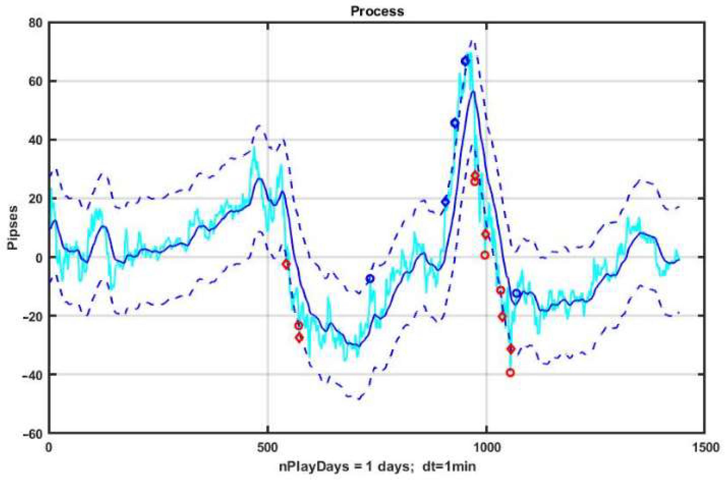
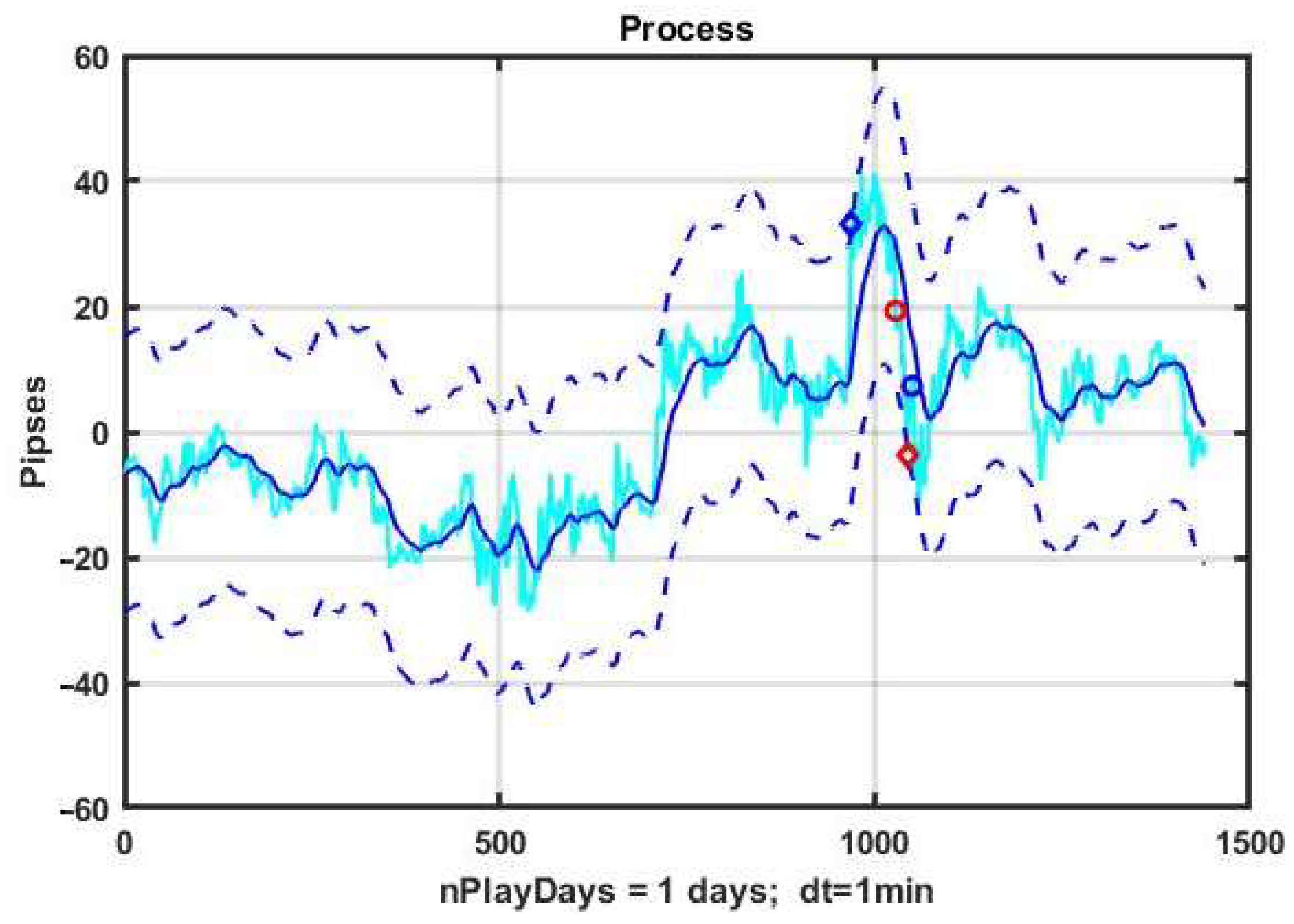
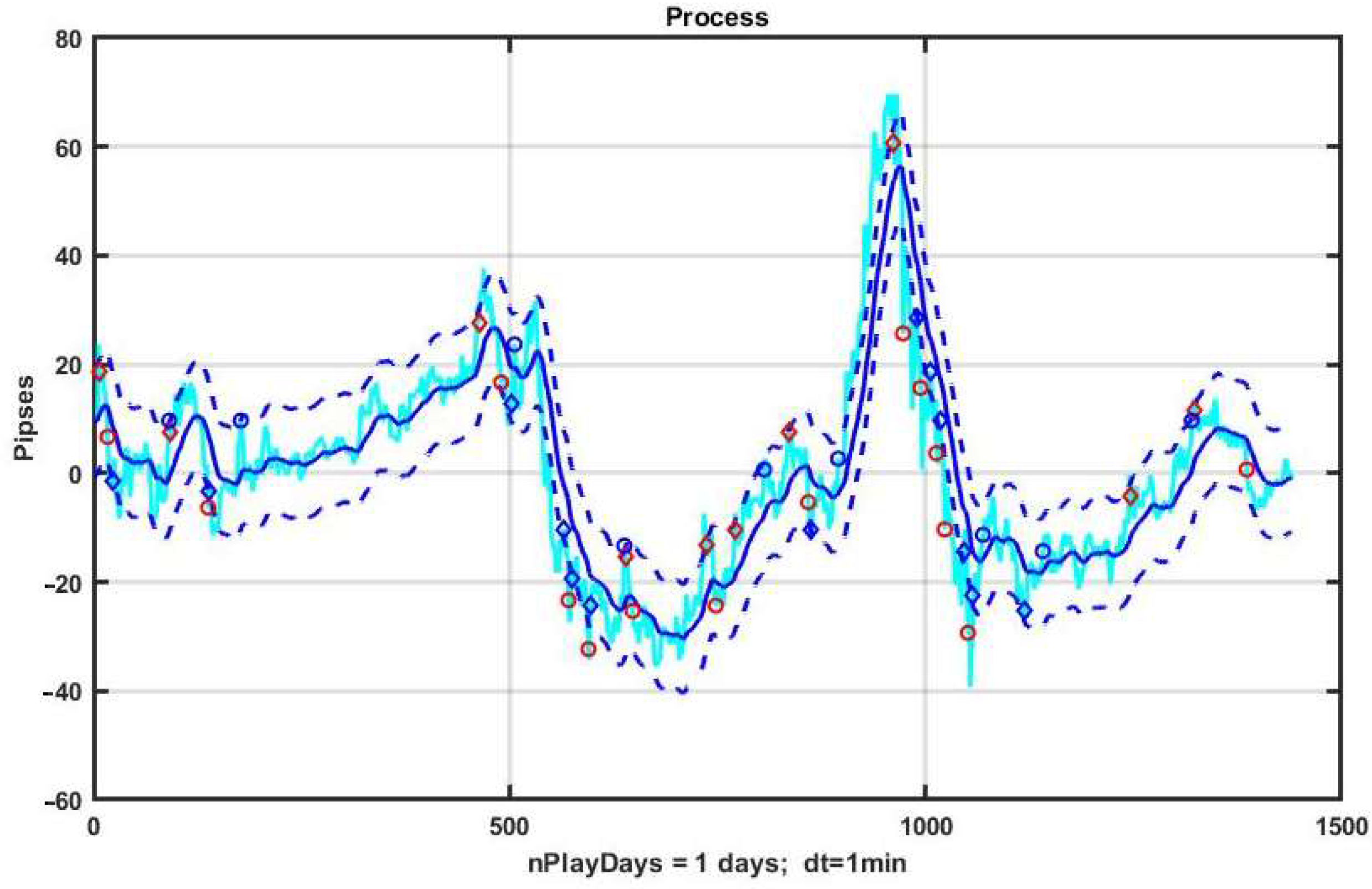
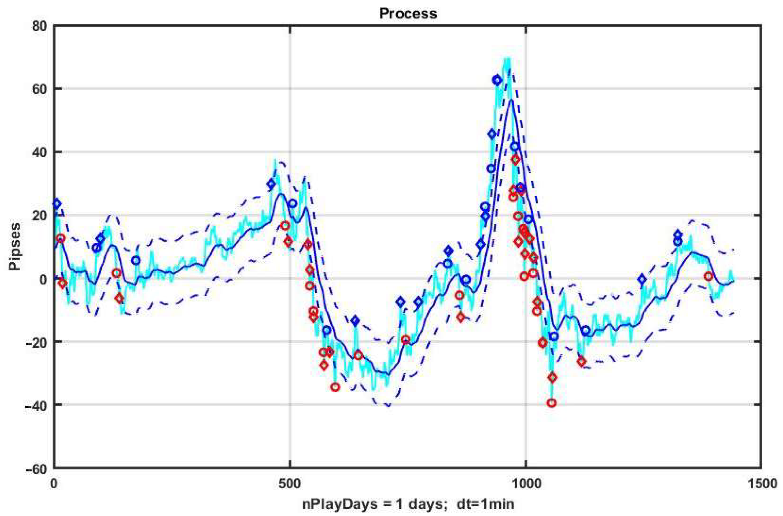
As a demonstration example, let us consider a day-long observation segment of EURUSD quotes shown in
Figure 1. The strategy consists in opening a position up or down when the process exits, respectively, beyond the lower or upper boundary of the channel.
Note that opening a position at the moment when the observed process leaves the channel can lead to a large negative drawdown, since the time and level of reversal of the observed process are unknown. Moreover, if the previous hypothesis about the emergence of a trend is true, then such a position opening can lead to a big loss. Therefore, it is more rational to open a position at a reverse intersection of the channel, which increases the stability of management, but, at the same time, makes a more modest gain.
The basic algorithm for controlling the movement against the trend is described by the following rules: Open Up is carried out under the condition (yk > xk − B) & (yk-1 < xk-1 − B), k = 2,…,n, and Open Dn − (yk < xk + B) & (yk-1 ≥ xk-1 + B), k = 2,…,n. The position is closed when either of the levels yclose > yopen + TP; yclose < yopen − SL are reached with Open Up or yclose < yopen − TP; yclose > yopen + SL with Open Dn.
An example of an alternative option for closing a position is the moment when the observed process crosses the conditional mean level xk, k = 1,…,n.
It should be pointed out that the presented algorithm is extremely “careful”, as in, the opening is carried out only when the asset price returns to the channel, and the expectation of profit relies on the fact that the compensation mechanisms of the market do not act instantly and are prone to a certain inertia. At the same time, the gain turns out to be quite small, but this provides protection against losses in the event of a systemic trend that takes the quotation far beyond the channel.
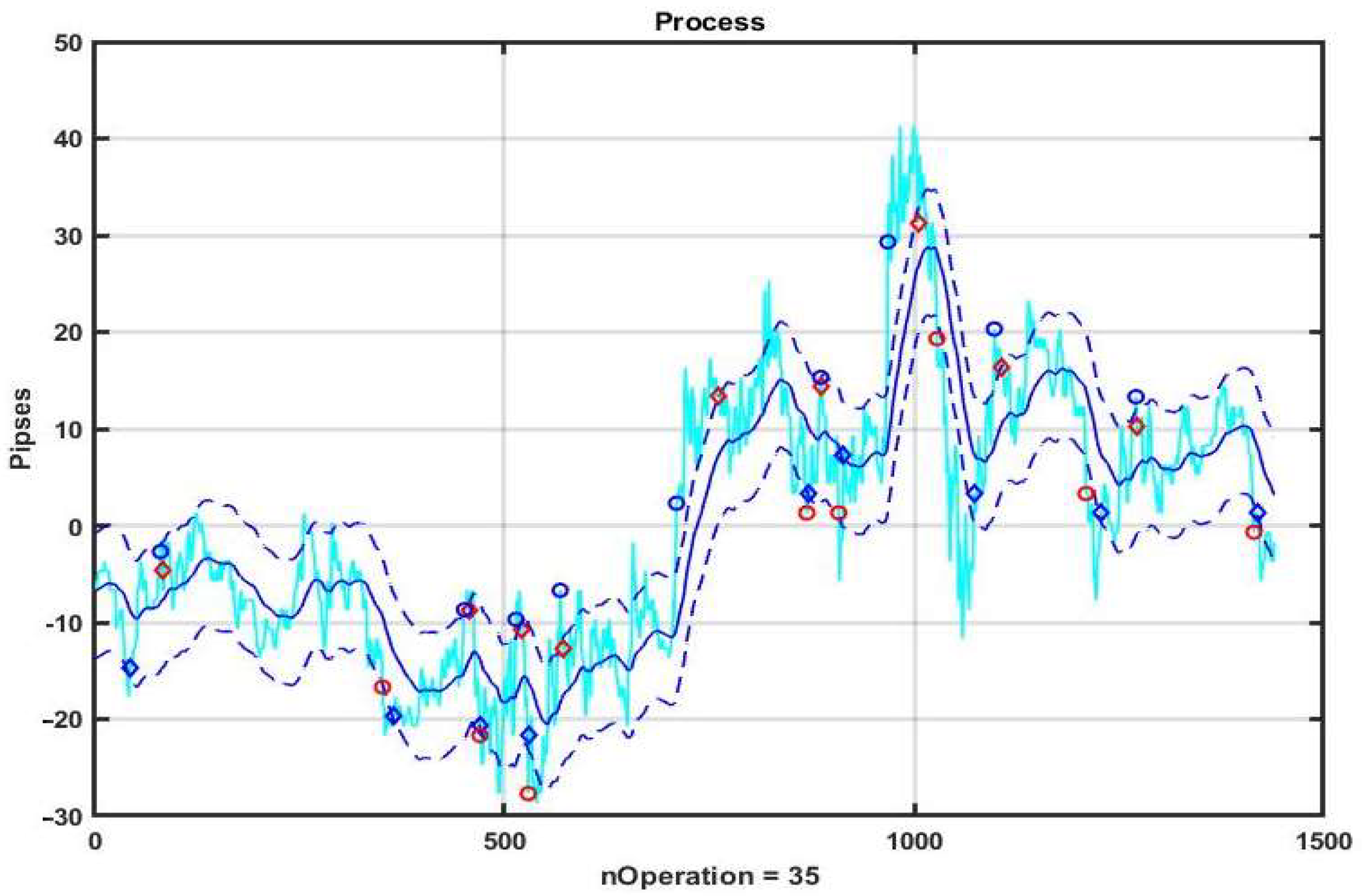
3. Results
Figure 1 illustrates the characteristics of a basic CSF strategy using a concrete implementation. We consider the quotes of the EURUSD currency pair as the observed process, and the management duration is one day (1440 min counts). The system component x
k, k = 1,…,n is formed by exponential filter (3) with α = 0.05. The width of the channel B = ±10 p is measured in points or pipses (p). The level of profit and the level of acceptable loss are TP = SL = 10 p.
On the chart, blue diamonds indicate the detection of an upward trend, red ones indicate a downward trend, and circles of corresponding colors indicate the levels of decision making about the quality of management.
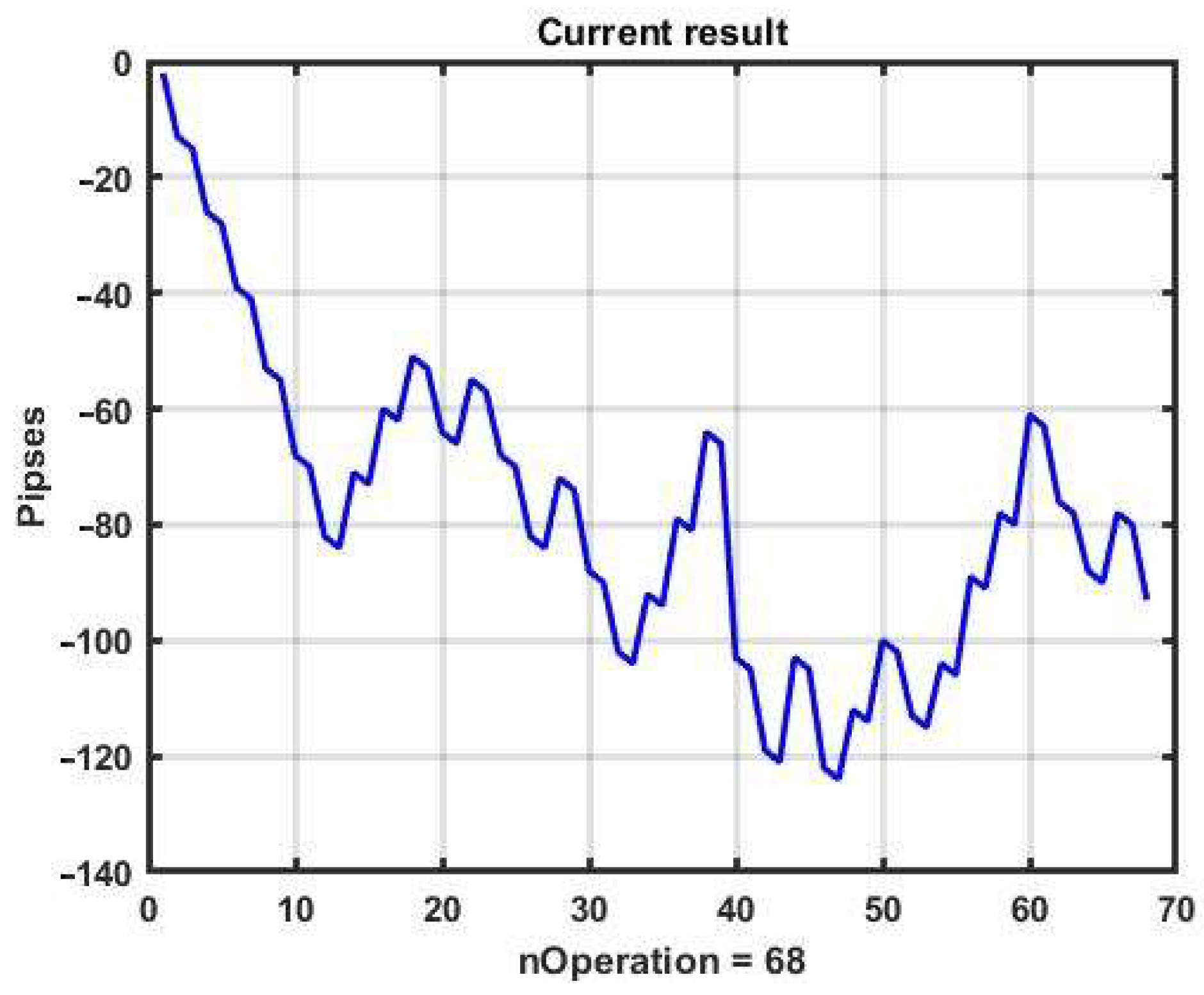
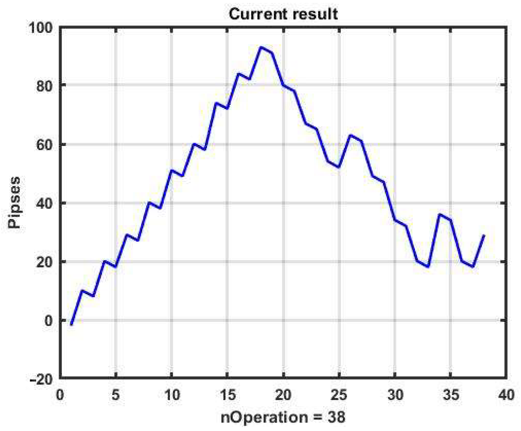
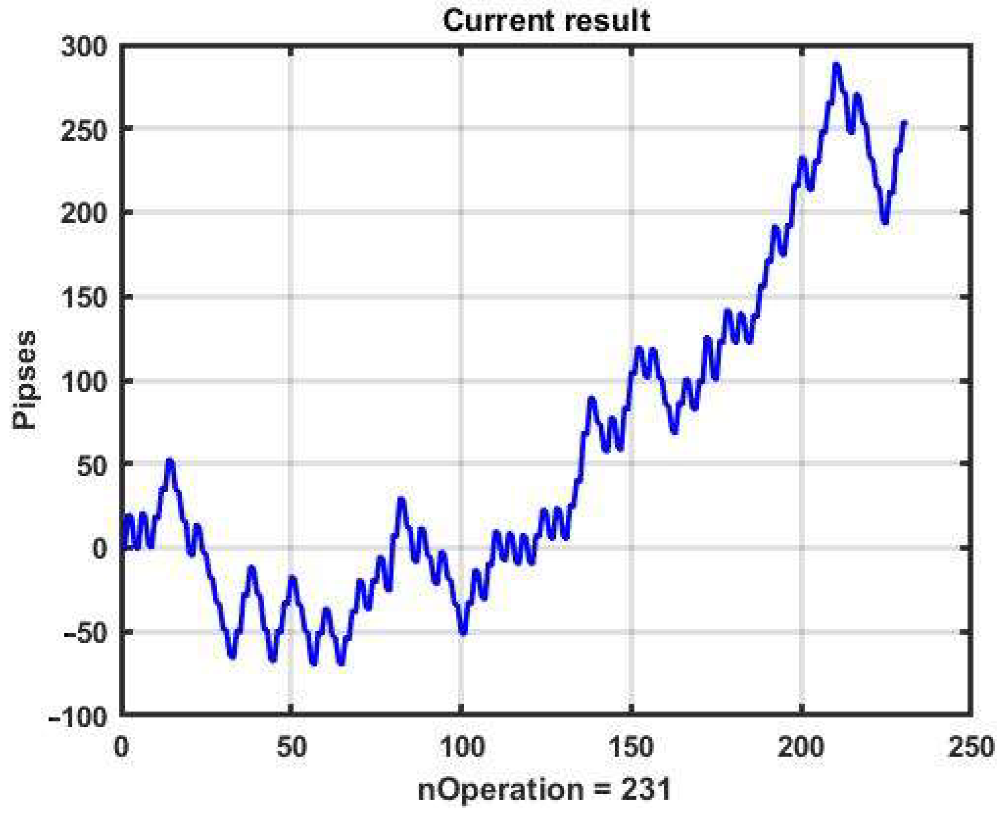
Figure 2 shows a plot of changes in the effectiveness of management (3) in the process of applying the channel strategy in the selected example. The result is obviously negative: the loss was −93 p per day.
The reasons for the loss are obvious. The presented forecasting technique can produce results only for areas with a strong, pronounced trend. For areas with weak local trends, this strategy only produces loss. Nevertheless, it allows for improvement via parametric fitting and introducing additional conditions into the management algorithm.
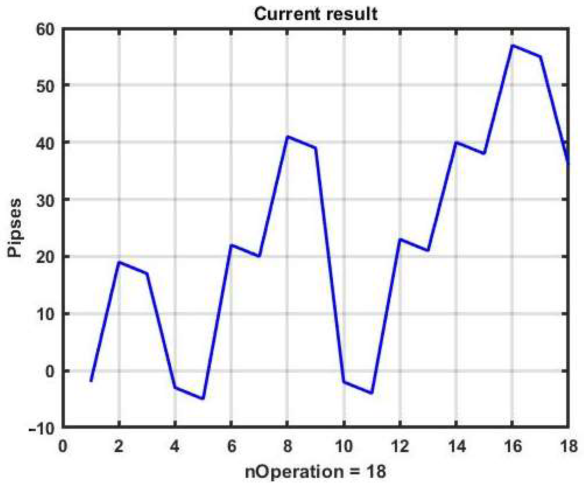
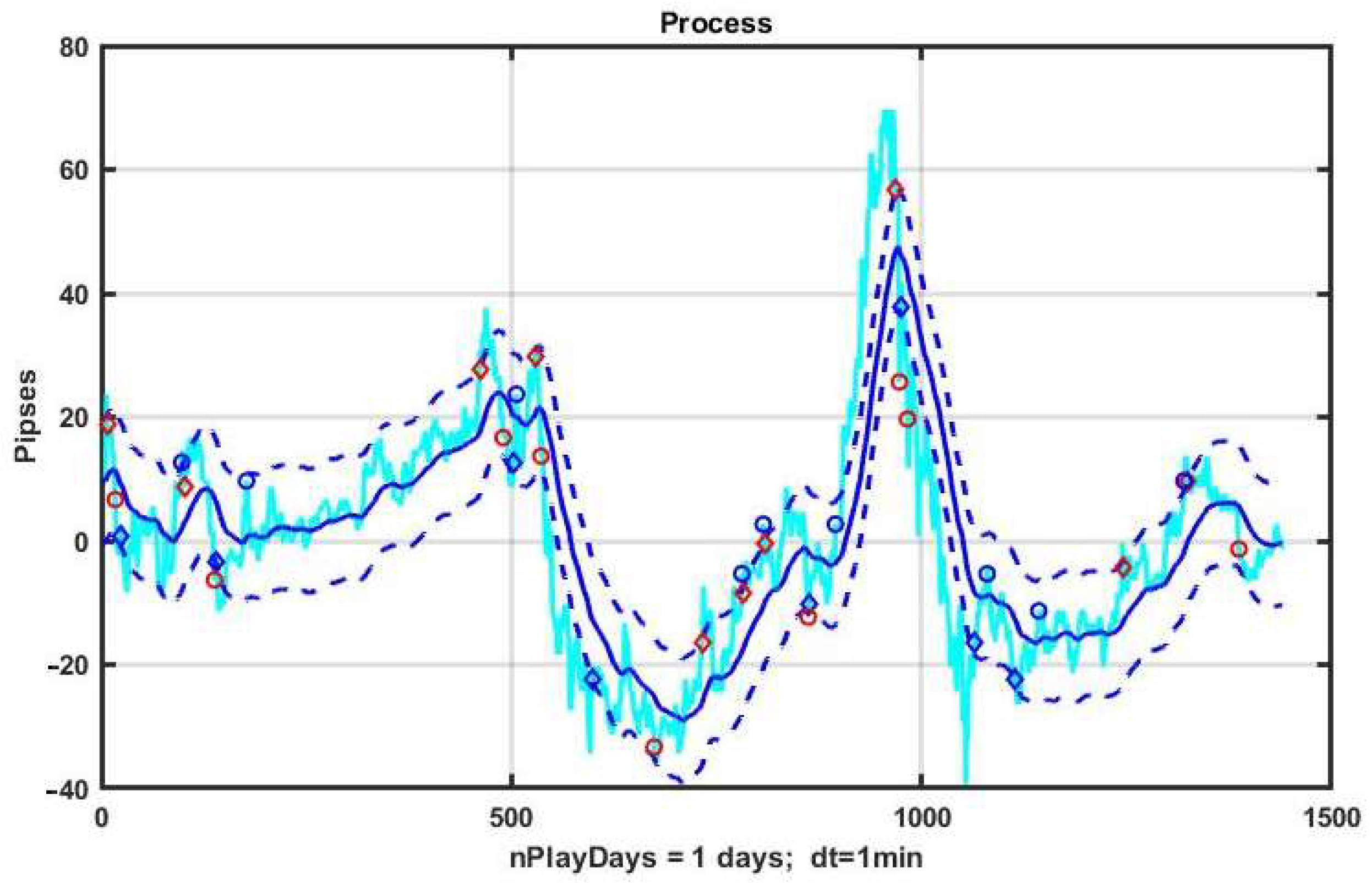
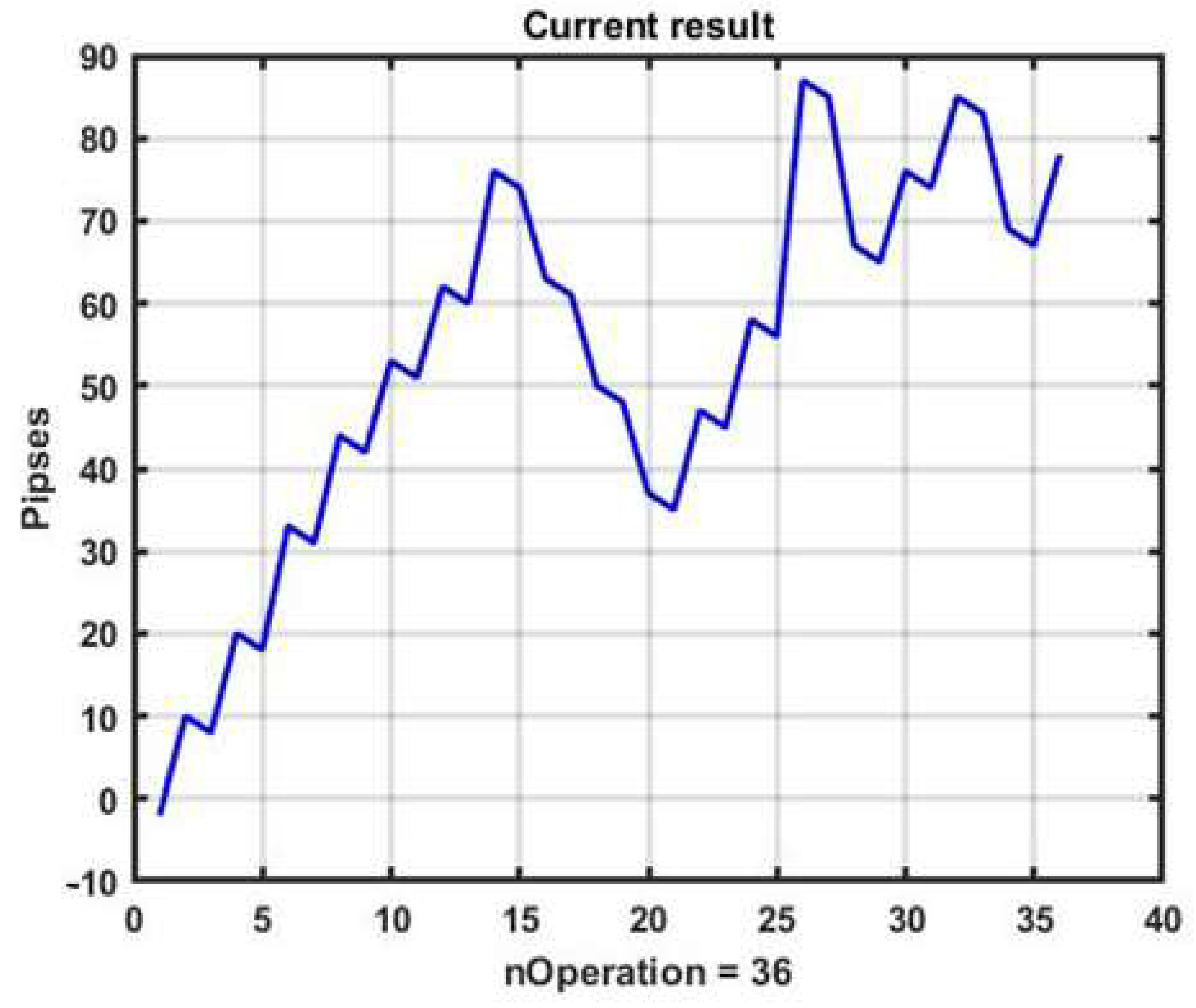
For example, increasing only the channel width up to B = ±18 p can make the management strategy at the same observation area profitable (see
Figure 3 and
Figure 4).
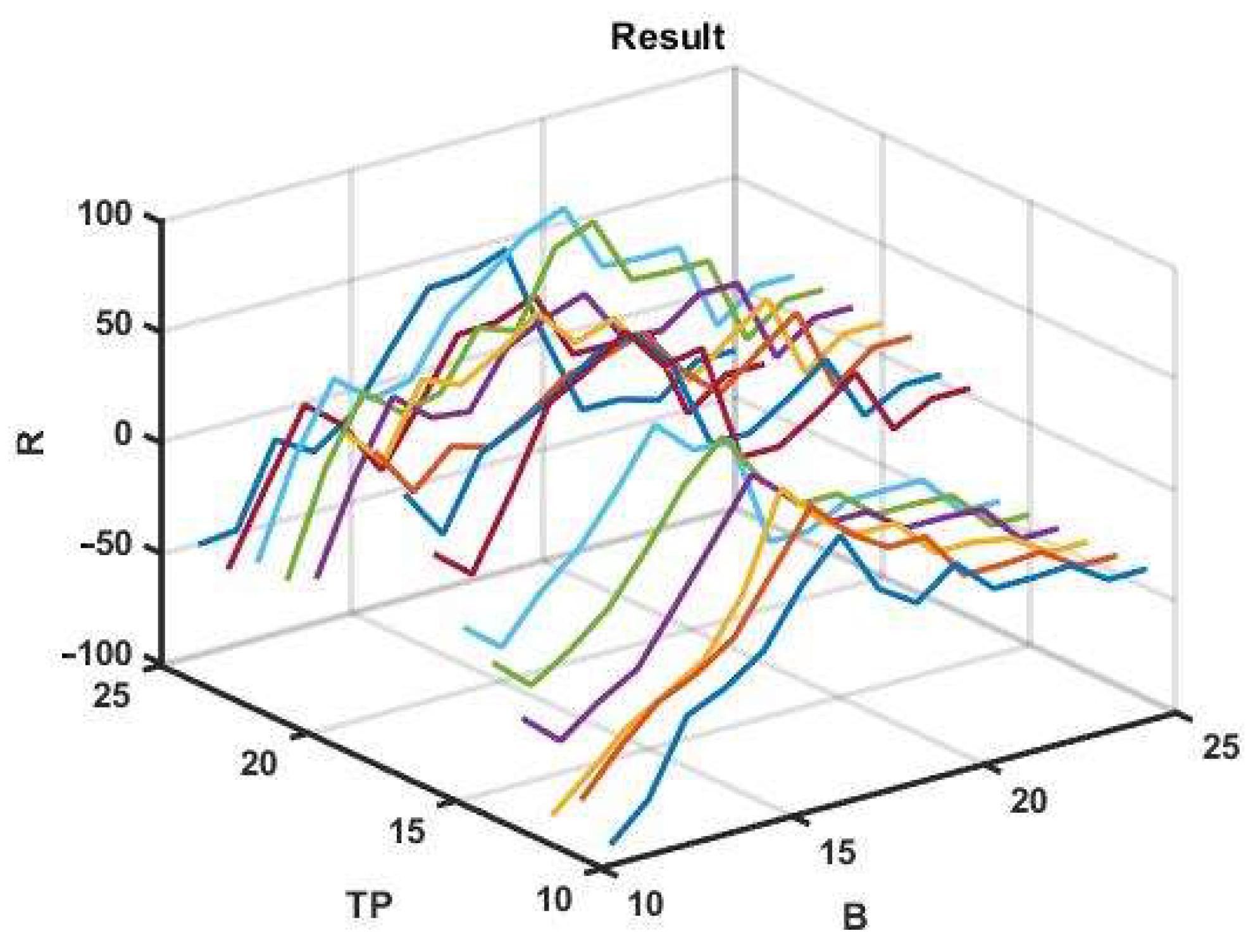
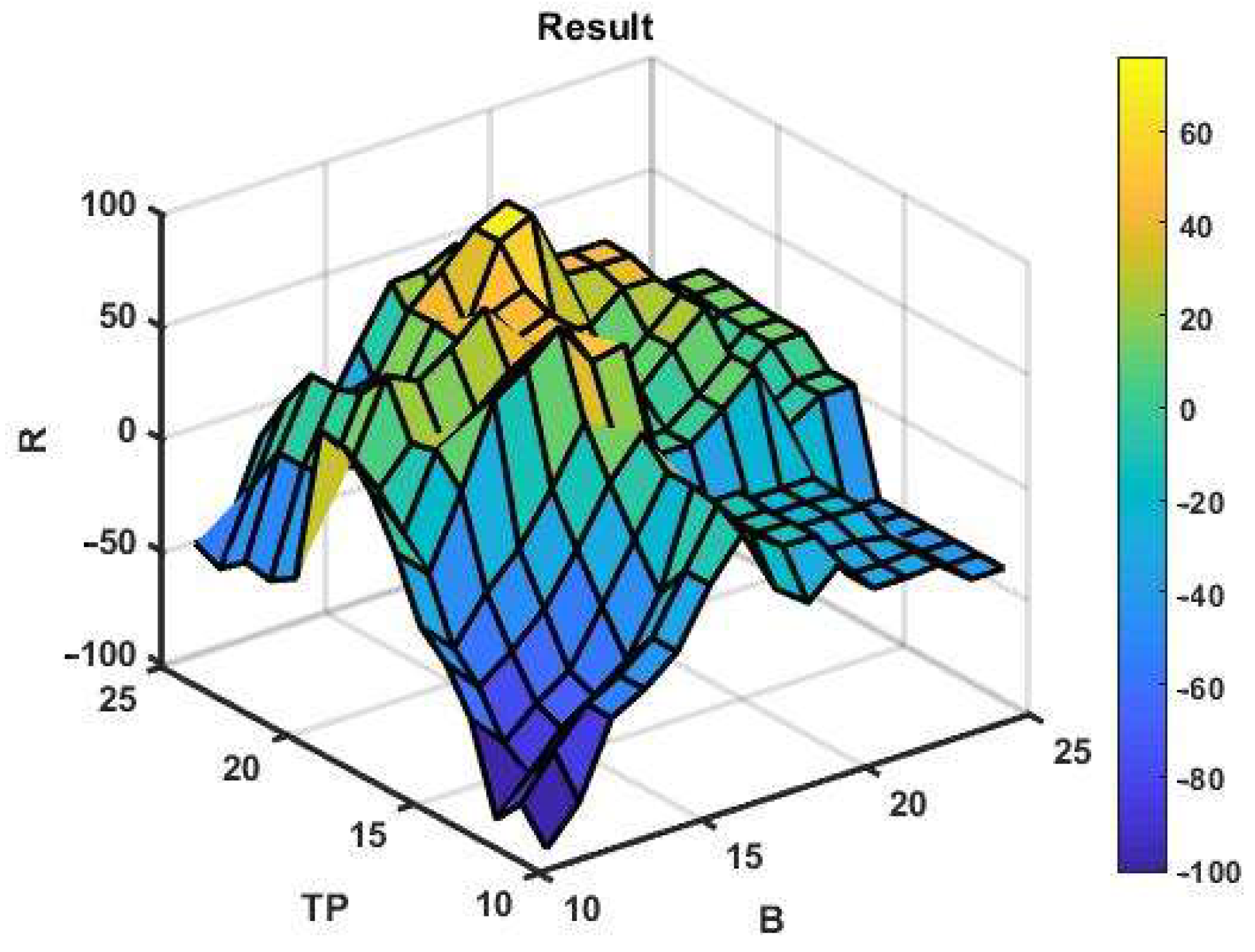
To assess the potential gain, we have initially used a brute force search for only two optional parameters in the ranges B = 11:1:25 and TP = 11:1:25. For the given values of the options, the best profit was R = 76 p with B = 19, TP = 22. Three-dimensional plots of the management results for the selected optional parameter ranges are shown in
Figure 5. The same plots with network approximation are shown in
Figure 6.
It is not difficult to see that the approximating surface is discontinuous with jumps in values even at minor variations in arguments. Thus, it can be concluded that the effectiveness of a channel management strategy based on movement in the direction of the trend is unstable. At the same time, parametric fitting based on retrospective data on a selected observation interval does not guarantee a positive result at the next subsequent time interval with the same parameters. An example of this is shown in
Figure 7. When using the optimal parameters for a selected observation interval for the next interval of the same duration, the result turned out to be negative and amounted to R = −29 p.
Repeated a priori optimization on the same area produced a result of only R = 5 p with the best option parameters being TP = 12, B = 19.
It should be noted that channel management can undergo various modifications, each of which makes sense for certain types of the observed dynamic process [
6,
7,
8], but none of them has a margin of stability that makes it possible to obtain a positive result on the whole variety of processes generated by market chaos.
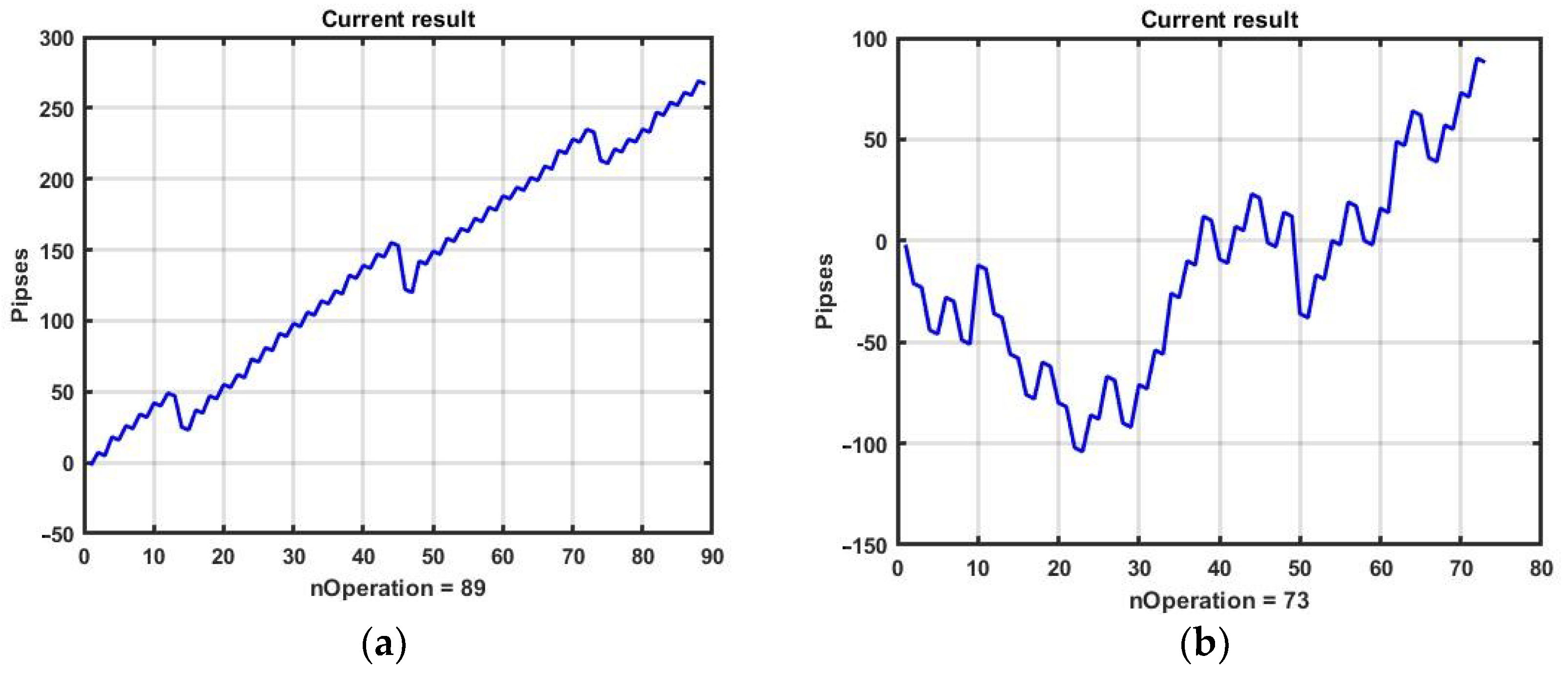
3.1. Evaluation of CSF’s Potential Performance
Let us consider typical versions of improving channel management strategies.
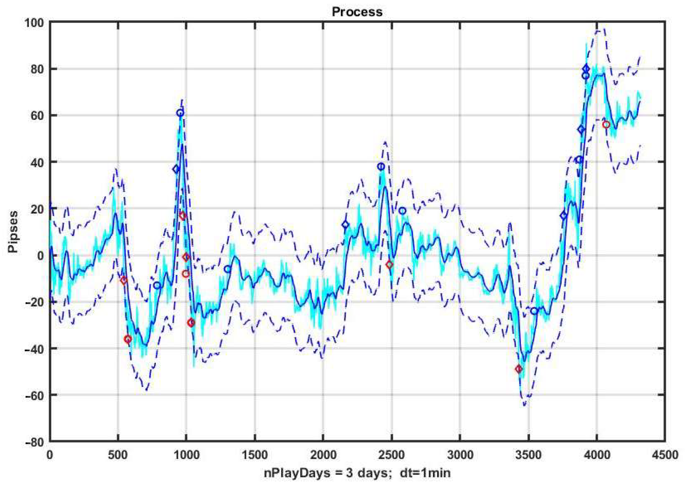
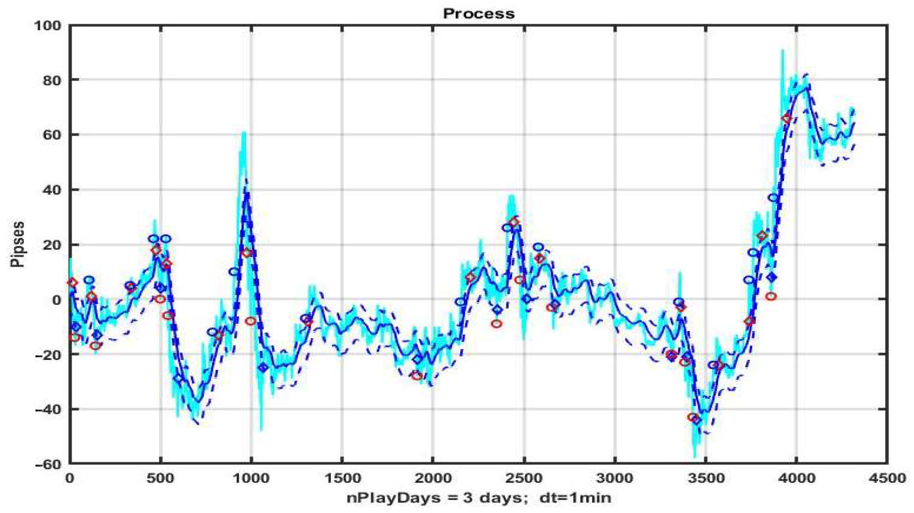
Figure 8 shows the results of management based on CSF on a three-day observation interval with pronounced areas of strong trends. On the basis of an a priori three-parameter optimization obtained by brute force search, we have identified best values of B = 19, TP = 22 and SL = 22, corresponding to exponential smoothing (1) with the transfer coefficient α = 0.05.
The example is profitable at R = 32 p; however, the result is unstable and even small variations in the structure of observation series definitely lead to a loss. Without a priori optimization, a trend-based management strategy almost always leads to a negative result. The rationale for this is given in studies of the inertia of chaotic processes in [
32].
Is it possible to improve the result by extending the vector of optimized parameters and using different values for the upper and lower boundaries of the channel? To solve this problem, we consider five-parameter optimization, including the filter smoothing coefficient α, the lower and upper channel boundaries B
Dn and B
Up, and the stop parameters TP and SL. Let us set the ranges of the selected parameters to α = 0.01:0.01:0.15, B
Dn, B
Up = 10:1:15, TP, SL = 10:1:15. For the selected three-day observation segment considered in the previous example, the best result of CSF was R = 166 p with the parameters P* = (α, B
Dn, B
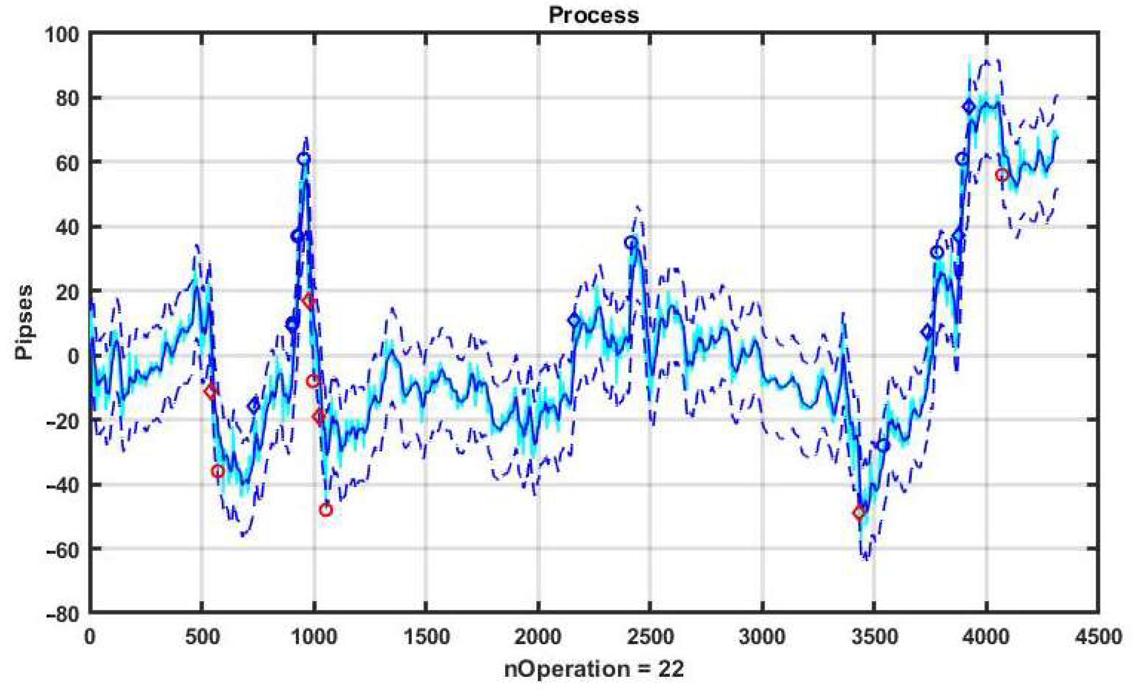
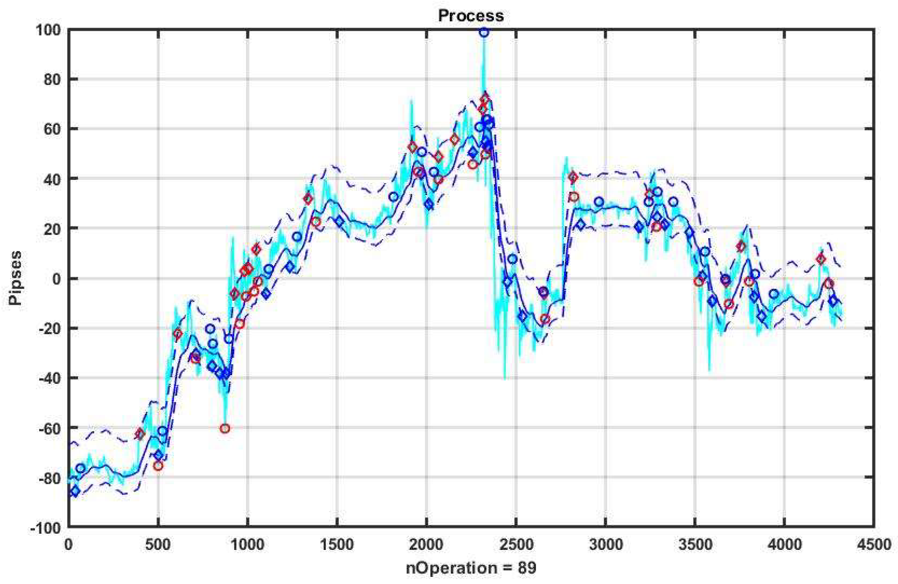
Up, TP, SL)* = (0.1, 13, 16, 23, 16). The implementation of the management strategy with the specified parameters at the selected observation interval is shown in
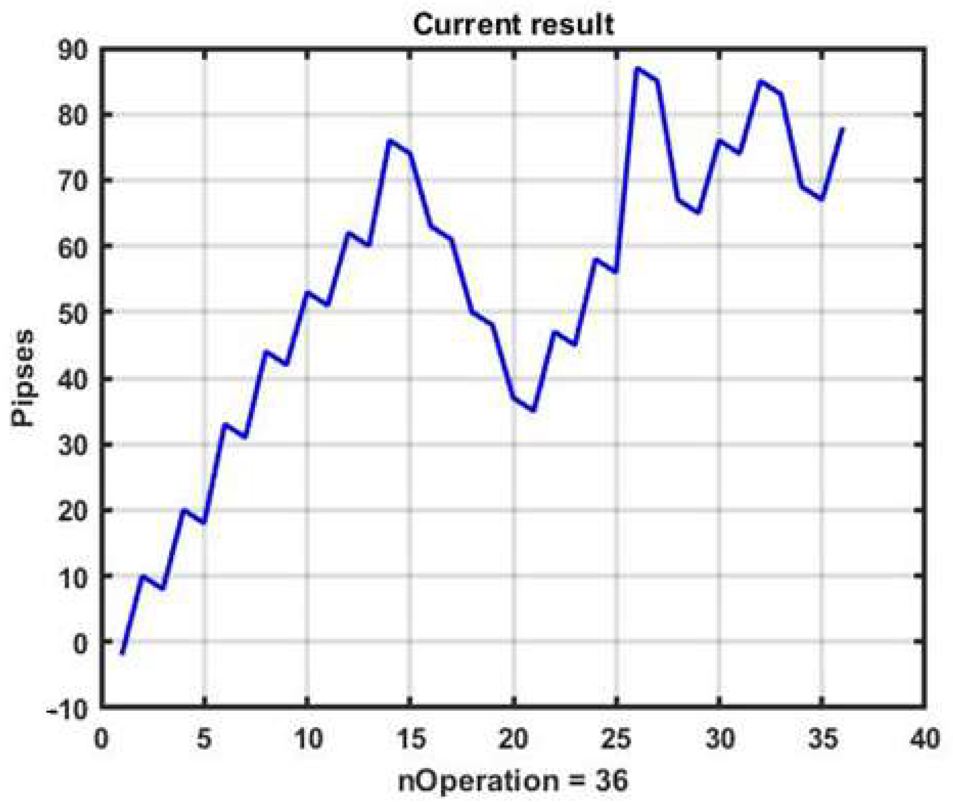
Figure 9, and the changes in the overall result of management are shown in
Figure 10.
Experiments show that R(P) is unstable: even minor deviations of the vector of optional parameters P from the optimum P* lead to a sharp decrease in the effectiveness.
It should be noted that brute force parameter optimization leads to an exponential growth of arithmetic complexity with an increase in the number of parameters or requirements for the accuracy of estimating optimal parameter values (i.e., decrease of the iteration step). This well-known fact can lead to serious problems in the construction of adaptive management strategies that sequentially estimate the optimal values of P.
Another important point is the asymmetry of management performance: among all the selected combinations, only 26% give a positive management result.
Attempts to increase the effectiveness of this strategy by improving system component isolation, the possibility of which was shown in the previous section, can only have an indirect effect, because during optimization it was compensated for by separately choosing the boundaries BDn, BUp and the filtration coefficient α. It is possible that this strategy will be more effective with separate dynamic adjustment of the upper and lower boundaries BDn, BUp, regarded as functions of the rate of change of the system component estimated on the sliding observation window BDn, BUp = F(xk − xk-τ), k = τ + 1,…,n. This issue requires additional research.
Figure 11 shows an example of CSB implementation. Similarly to the previous example, the system component x
k, k = 1,…,n is evaluated as the result of the smoothing performed by exponential filter (3) with α = 0.05. The initial values of the option parameters are: channel width B = ±10 p, take profit level TP = 10 p, acceptable loss level SL = 10 p.
From the above figure, as well as from the plots of changes in the result due to the management strategy (
Figure 12), it can be seen that the adopted asset management produces stable gain on weak trends (see the first third of the plot). However, when strongly pronounced trends occur, this strategy leads to incorrect decisions.
To evaluate the effectiveness potential of the proposed management strategy a posteriori, we apply a brute force search to optional parameters, as discussed above. We iterated over the values of three control parameters in the ranges α = 0.01:0.01:0.1, B = 10:1:25, TP = 10:2:25 on a single-day observation segment shown in
Figure 11. As a result of comparing 880 combinations, we found that the optimal values of the option parameters were α* = 0.03, B* = 10 and TP* = 10, i.e., the parameters selected in the example were either close to or coincided with the best. However, the probability of a positive outcome was low: out of 880 parameter combinations, only 137 provided a positive result. The optimal profit value for the selected combination option was R* = 78 p.
An example implementation of a CSB management strategy with an optimal combination of optional parameters is shown in
Figure 13, and the corresponding plot of changes in performance is shown in
Figure 14.
It should be noted that a number of losing decisions are explained not by the overall decision quality, but by a significant bias that occurs during the filtration process (3) during the isolation of the system component x
k, k = 1,…,n. In
Figure 1,
Figure 8,
Figure 11 and
Figure 13, it can be easily seen that when a strong trend occurs, the system component formed by the smoothing filter lags behind the observation process, which leads to a shift of the entire channel and incorrect use of the management strategy concept itself. Hence, natural suggestions arise for improving the management by modifying the sequential filtering procedure and dynamically changing the size of the lower and upper channel boundaries.
3.2. Evaluation of CSB’s Potential Performance
Let us compare the estimates of the potential effectiveness of CSF and CSB management strategies on the same three-day observation interval. We will retain the same set of ranges for optional parameters, α = 0.01:0.01:0.15, B
Dn, B
Up = 5:1:15, TP, SL = 7:1:15. Using a brute force search, the best result of the CSF strategy was R = 166p with P* = (α, B
Dn, B
Up, TP, SL)* = (0.1, 13, 16, 23, 16). The implementation with the specified parameters at the selected observation interval is shown in
Figure 11.
The CSB’s best result for the selected observation area was R = 250 p, corresponding to P* = (α, B
Dn, B
Up, TP, SL)* = (0.03, 8, 5, 17, 17). Its implementation is shown in
Figure 15.
Comparing the two channel strategies with optimal vectors of optional parameters allows us to draw the following conclusions:
Both strategies have profitable decisions, but the result in both cases is not stable and small changes in control parameters can lead to a radical decrease in gain;
Management against the trend needs a higher level of smoothing, which activates the opening of a position on a sideways trend and reduces the frequency of management in areas with a strong trend. On the contrary, playing by the trend requires reducing the degree of smoothness, which makes it possible to more effectively detect a strong trend and activate management in these areas of observation;
The width of the channel when playing against the trend is significantly, two to three times, smaller than in the opposite case, which increases the frequency of opening in horizontal quotation sections. Obviously, in both cases, the choice of channel width is related to the degree of volatility, as a measure of which, for example, the standard deviation (SD) of observations relative to the system component can be used.
Due to the paper limit, we will illustrate our further research with numerical results based on the use of the CSB management strategy.
3.3. Parametric Stability of Optimal Solutions
In order to check the stability of the solutions produced by the considered a posteriori determination of optimal parameters, we will consider another three-day observation section, following the one presented in
Figure 15, containing discontinuous sections of quotation changes.
The result of optimization using CSB was R = 267 p with the parameters P* = (α, BDn, BUp, TP, SL)* = (0.02, 7, 14, 8, 19).
Now let us evaluate the effectiveness of the same strategy at the same observation segment, but with the parameters optimal in the previous three-day interval. Comparisons of management performance with the CSB strategy in the example shown in
Figure 15 with optimal parameters (left) and using the same parameters in the subsequent three-day observation interval (see
Figure 16) are shown in
Figure 17.
It is easy to see that the gain decreased by about three times (R = 88 p), and in the process of management, the result decreased to a loss of 100 p.
Let us consider the stability of the CSB strategy performance in response to particular variations of individual parameters. To this end, we will evaluate the effectiveness on the same three-day time interval as in the previous experiment, but with deviations of the optional parameters B
Dn, B
Up, TP and SL from optimal in the range P* ± 0.1 P*, and α in range α* ± 0.5 α*. The range of changes was divided into eight steps, i.e., four steps in each direction from the optimal value of the parameter.
Table 1 presents the changes in performance for this strategy.
3.4. Examining the Dynamic Stability of Optimal Solutions
From the above data, it can be seen that the management has a certain margin of stability, i.e., small changes in the values of the option parameters do not lead to an abrupt change in performance. This conclusion leaves hope for the possibility of implementing an adaptive approach, when the optimal setting at the previous stage is used as the set of optional parameters at the subsequent observation site.
However, a more accurate conclusion requires an analysis of the stability of the control with simultaneous variations of groups of parameters. In addition, it is necessary to examine this issue in dynamics, i.e., taking into account the time shift of the observation area.
For clarity, let us consider the process of asset management with the CSB strategy during a single day of observation, shown in
Figure 18. With brute forcing, we obtain a vector of optimal parameters P* = (α, B
Dn, B
Up, TP, SL)* = (0.03, 7, 6, 11, 12), the use of which produces gain R = 164 p.
Let us consider the question of how stable the obtained vector will be during the next two days of management.
Figure 19 shows graphs of three days of observation (separated by days by red circles), from which it can be easily seen that the relatively smooth dynamics of the first day, on which parametric optimization was carried out, are not at all similar to the dynamic data structures of the two following days. The second day is characterized by a decline followed by a strong positive trend, the third day is characterized by an uneven positive trend (growth).
Thus, the settings produced on the first day of observation will obviously produce only loss for the next two days. In this example, the loss was R = −90 p on the second day and R = −57 p on the third day. Thus, the assumption about the parametric instability of the channel strategy, which is obvious to all practicing traders, is confirmed.
Note that the first day, which was used for the training, i.e., determining the best values of optional parameters, was quite “comfortable” for a CSB-type management strategy. The corresponding observation segment was a sideways trend with small variations. Naturally, when strong trends occur, management with parameters optimal for a sideways trend turns out to be losing.
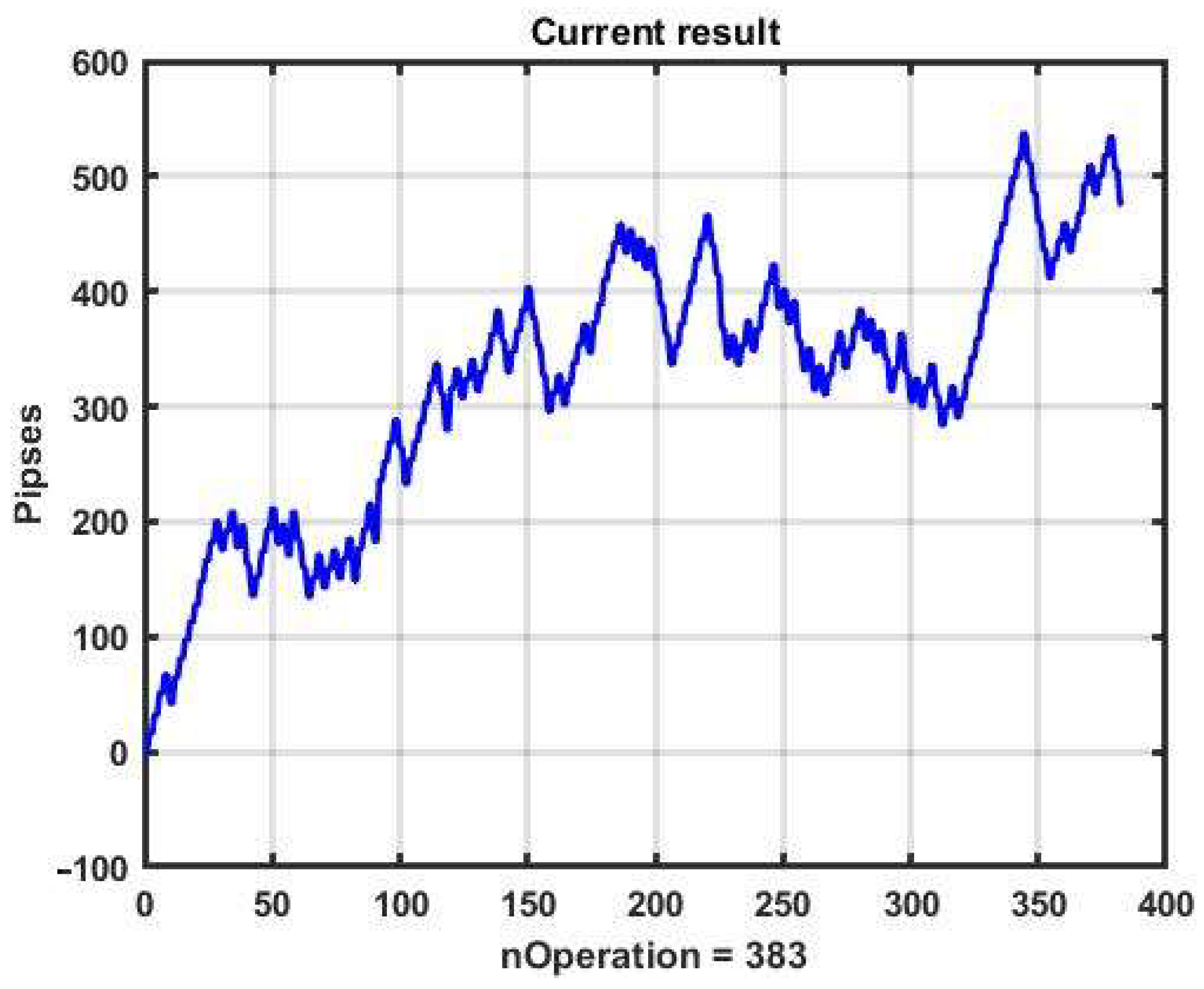
Consider a channel management strategy with enhanced resistance to variations in the dynamics of observations: a model with parameters optimal over a large observation interval. In the example, we examine an observation interval of 15 days. This area contains a large variety of dynamics: sideways trends with different heights, areas of slow and abrupt increases and decreases, jumps, etc.
We optimized the parameters via brute force on the following ranges: α = 0.01:0.01:0.15, B
Dn, B
Up = 5:1:15, TP, SL = 7:1:15. The test result of using CSB was R = 475 p with P* = (α*, B
Dn*, B
Up*, TP*, SL*) = (0.02, 6, 8, 17, 21). The performance of the management strategy with specified parameters at the selected observation interval is shown in
Figure 20.
Using these parameters separately on each observation day, we obtained R = 456 p, which is quite close to the previous result of optimizing for the entire 15-day observation area. Let us consider how effective the parameters P* are in the subsequent 10-day observation interval that does not intersect with the training data interval. The total sum of one-day results in this case is R = 51.
We chose the same large observation interval of 15 days as for the CSB strategy, preserving the same ranges for the following parameters: α = 0.01:0.01:0.15, BDn, BUp = 5:1:15, TP, SL = 7:1:15. Their best values, P* = (α*, BDn*, BUp*, TP*, SL*) = (0.1, 11, 14, 16, 13), were obtained by brute force search.
Figure 21 presents the performance of the strategy. The best result was R = 252 p, which is significantly worse than the CSB’s result with optimal parameters at the same interval.
Following the proposed method of stability analysis of the obtained result, let us consider how effective the found optimal parameters are in the subsequent 10-day observation interval that does not intersect with the training interval (
Figure 21). The total sum of one-day results in this case is R = −534, which indicates low efficiency and pronounced dynamic instability of this management strategy.
4. Discussion
Given studies clearly indicate the theoretical applicability of channel strategies to the task of speculative management of financial instruments in conditions of market chaos. However, their practical implementation faces the problem of weak predictability of changes in the value of market assets, which, combined with low statistical stability of management in the conditions of market chaos, leads in most cases to negative results.
The obvious consequence of this conclusion is the need to extensively modify channel strategies to increase their resistance to dynamic variations in the structure of observation series.
The traditional approach to improving the stability of system functioning in conditions of uncertainty is based on various adaptive computing schemes. For systems with a high level of dynamic uncertainty characteristic of market pricing processes, it is natural to use sequential adaptation on a sliding window of application adjacent to the current time moment. At the same time, it is possible to use both nonparametric adaptation, which modifies the structures of the observation model, and traditional parametric adaptation.
It should be noted that the parametric adaptation based on posterior brute force optimization of the values of the optional parameters, in conditions of strong variability characteristic of quotation dynamics, may not be feasible. This is due to the rapid growth of the time complexity with an increase in the number of parameters. Due to this, it is advisable to utilize suboptimal optimization with significantly lesser computational demands.
It should be pointed out that any kind of adaptation of decision-making algorithms in conditions of chaotic dynamics is a very difficult problem. The market information space is an unstable immersion environment. As shown previously [
32], similarity of aftereffects does not follow from the geometric or correlational similarity of two multidimensional situations. As a consequence, an effective solution on the previous sliding observation interval does not guarantee a quality solution on the current observation window. Nevertheless, the studies of the stability of solutions presented in the article retain hope for the possibility of creating fast self-organizing systems, for example, based on evolutionary optimization technologies [
33], allowing to increase the stability of channel management.
The main alternative to adaptation is reducing the sensitivity of decision-making algorithms to variations in the dynamic and statistical characteristics of observation series. The robustification of forecasting algorithms and management decisions is based on the search for the best options for the least favorable variants of initial data implementation [
34]. However, as already noted, there is no similarity of aftereffects for such observation segments in the conditions of stochastic chaos. In this case, a uniform decrease in the quality of management does not follow from a consistent decrease in the quality of estimation and forecasting algorithms. In other words, the quality of the best solution for the worst case of the source data under these conditions will not be stable for other parts of the source data.
Nevertheless, this requires numerical validation, and even if the assumption is confirmed, it is of interest to use robustification in combination with other methods to increase the stability of proactive management strategies.
Another possible solution is to switch to multi-expert decision-making systems (MES), involving both strategies in the management [
35]. Such an approach can produce many possible solutions based on consensus and compromise.
As an example, consider an expert arbitrator who has information about the general mood of the market. In particular, such a software expert can be implemented as an automatic text analyzer that evaluates market sentiment by identifying the required knowledge from analytical reports circulating on the web [
36]. Based on the decision of the expert, one of the two channel management strategies is selected, the most consistent with the expected dynamics of the quotations.
Apparently, the best results of management in chaos should be expected from composite algorithms and multi-expert systems that widely use external add-ons such as fundamental analysis or the results of technical analysis of alternative markets.
Generalizing the abovementioned conclusions, the following directions of increasing the stability of management seem to be worthy of consideration:
Dynamic adaptation of decision-making algorithms with the choice of the best parameters on sliding observation windows;
Robustification, i.e., reduction of the sensitivity of solutions to changes in the dynamic characteristics of the observed processes;
Improvement of management based on more flexible computational schemes for selecting boundaries of a channel or several channels and decision-making algorithms;
Structural adaptation, for example, based on switching between management strategies as a reaction to changes in the dynamic properties of the system component of the observation series;
Self-organization based on artificial intelligence, which independently creates strategies that are not contained in the source code of the management program;
The use of composite algorithms combining the capabilities of robustification and adaptation in management decision making;
The use of external add-ons that carry information exogenous to technical analysis on expected trends of the considered financial instrument and market mood in general.
The outlined issues constitute the subject of our further research.


