1. Introduction
The problem of effective control in non-stationary immersion environments appears in a large number of applications. They are meteorology, the control of turbulent hydrodynamic flows, the stabilization of the state of non-stationary technological processes, asset management in capital markets, etc. The intricacy here is due to the unstable nature of the observed processes described by models of nonlinear chaotic dynamics [
1,
2,
3,
4,
5,
6,
7,
8,
9,
10]. Non-stationarity means that different observations have means, variances, and covariances that change over time. The non-stationary behavior can be a trend, a cycle, a random walk, or a combination of these. Non-stationary data is generally unpredictable and cannot be modeled or forecasted. Results obtained using non-stationary time series can be misleading because they may indicate a relationship between two variables when in fact there is none. For a better introduction to the subject, see the following Investopedia article [
10].
High volatility and low predictability of chaotic processes significantly complicate the effective use of well-known control stabilization techniques based on traditional methods of adaptation and robustification. In particular, adaptive technologies turn out to be too inertial to close the feedback loop in time. Increasing the sensitivity of feedback leads to a high level of statistical errors of type II (“false alarms”). Robust control methods [
11,
12,
13,
14,
15] focused on solutions with reduced sensitivity to statistical and dynamic variations of the observed process in the conditions of a basic model significantly lose effectiveness compared to optimal a posteriori versions.
A control strategy based on sequential dynamic optimization of the control model in chaotic dynamics, as will be shown in this paper, also faces a number of well-known problems. Here we have, for example, bruteforcing control parameter values with a given step that determines the accuracy of the solution, exponential increasing amounts of calculations with an increase in the number of model parameters. Taking into account the high variability and unsteadiness of the observed process, the number of parameters of the optimized control model should not exceed five or six even for modern techniques. Hence, there is a need to study new techniques of sequential dynamic optimization of the control model based on suboptimal computational schemes.
In this paper, we use an observation series of currency pairs in the Forex market as a testing ground for studying the effectiveness and stability of control algorithms in chaotic immersion environment. Dynamic chaos in an observation series violates the fundamental premise of the repeatability of experiments under identical conditions. In particular, two geometrically similar observation segments in conditions of chaos may have completely different aftereffects [
16,
17]. As a result, traditional statistical data analysis technologies and control algorithms based on them are ineffective. In our studies, the choice of channel control strategies is determined primarily by their accessibility and interpretability.
This article considers the possibility of applying sequential optimization based on the method of evolutionary modeling in conditions of stochastic market chaos [
18,
19,
20,
21] etc. The method is based on the Darwinian concept of evolutionary self-organization and the theory of random search.
2. Methods
2.1. Observation Model and Problem Statement
A significant difference between the presented work and traditional studies in the field of asset management is their focus on the Wald’s additive observation model [
22,
23,
24]
where x
k, k = 1, …, n is the system component used in the process of making management decisions (i.e., open, close or retain current position), and v
k, k = 1, …, n is the noise.
Currently, the prevailing point of view is that in market situations, the system component x
k in (1) is modeled as an output signal of a nonlinear system observed in the conditions of non-stationary and non-Gaussian interference v
k (dynamic chaos model) [
5,
6,
7,
8,
9,
10,
11,
12,
13]. Lyapunov functions [
25] and identification methods based on higher-order spectra [
26] are used in order to substantiate such problem statements. There is a large area of research on the direct reconstruction of stochastic differential equations [
27,
28] for the model (1). Other points of view are based on nonlinear transformations of the y
k process, and, for example, on investigating fractal properties of the process trajectory [
29,
30,
31].
Sequential filtering of the initial observation series y
k, k = 1, …, n is usually used to isolate the system component x
k, k = 1, …, n from (1) in real time. For this purpose, we utilize an exponential filter [
32]:
with a discounting coefficient α ∈ [0.01, 0.3]. This range is our empirical finding for the Forex market. Simultaneously, it is possible to select α adaptively so it better corresponds to features of considered data. This filtering technique is not the best one, because an increase in the smoothing effect with a decrease of α leads to a significant bias of the generated estimates. However, it produces a satisfactory result for the considered examples, while also providing simplicity of interpretation of the extracted system component.
Note that the conventional statistical observation model is based on the assumption that its system component is an unknown deterministic process, and its noise component is a stationary random process with independent increments [
33]. Such a model was used in a wide class of trend analysis-based management strategies [
34,
35,
36,
37], though all of them are not resistant to possible dynamic variations in the process of changing quotes. One of the reasons for the unfeasible effectiveness of these trend indicators is the intrinsic inadequacy of the statistical approach for a chaotic observation series.
The main difference of the proposed model (1) is that its system component x
k, k = 1, …, n is modeled as an oscillatory non-periodic process with a large number of local trends. This description indicates the possibility of interpreting this process as an implementation of the dynamic chaos model [
5,
6,
7,
8,
9,
10,
11,
12,
13]. Its second distinctive feature is the noise component v
k, k = 1, …, n being interpreted as a non-stationary random process described by an approximate Gaussian model with fluctuating parameters. In particular, correlations and spectral characteristics of this process change significantly over time [
23,
24].
The indicated features of observation series described by (1) violate the conditions of applicability of traditional statistical methods. In this case, numerical studies are the only approach to analyze the effectiveness of the developed management strategies. The statement of the asset management problem essentially coincides with the traditional formalization of the task to maximize the gain in the process of trading or investing capital.
Let yk = xk + vk, k = 1, …, n be a sequence of observations corresponding to a given time interval of asset management T = nΔt, where Δt is the selected interval between time counts. During the specified time, M operations are carried out in the trading process, each being determined by their start and finish (kopen, kclose)j, j = 1, …, M.
The trading problem can be thus formulated as follows: select a management strategy S and construct a sequence of actions u
j, j = 1, …, M to obtain maximum profit G(S):
In the simplest case, each management strategy is defined by the rules that determine the time of opening and closing a position (kopen, kclose)j, j = 1, …, M, and, in some cases, the lot size. The sum of the operation results at the k-th step Gk(S) becoming smaller than the trader’s available deposit G0 means the management process resulted in complete loss.
The approach to determining the start time of an operation (the so-called “position opening”) is the defining characteristic of a management strategy. The operation can be finished (a “position” can be “closed”) when a specified profit level (TP, “take profit”) or loss level (SL, “stop loss”) is reached, or according to some different rules that could be more flexible.
This paper examines the technique of sequential evolutionary self-organization of the management strategy in the conditions of market chaos. Due to this, the simplest control schemes are used as basic control strategies, which makes it easy to visualize and interpret the obtained results. In particular, we used the so-called channel strategies [
4,
34,
35,
36,
37]. Let us consider the simplest approaches to constructing such a strategy.
2.2. Channel Asset Management Strategies
We have a series of the trading asset’s quote observations being modeled by (1). Let us define a “channel” as a range of observation values constrained by y
k = x
k ± B, k = 1, …, n [
33]. Variations inside the channel |y
k − x
k| = |δy
k| ≤ B, k = 1, …, n, are fluctuations that do not contain an obvious trend, in which case, the process can be referred to as a sideways trend or a flat. Channel width B can be selected depending on various considerations. It usually lies in the range from s
y to 3s
y, where s
y is the estimate of the standard deviation (SD) δy
k, k = 1, …, n. In general, the choice of channel width depends on the nature of the data and the specificity of the selected management strategy. In some cases, the channel width may be some variable value B
k = B
k(y
k), k = 1, …, n.
The observation series value yk, k = 1, …, n that breaks out of the channel is interpreted as the emergence of a trend in some management strategies. In the case of managing assets according to the trend direction, such events give rise to a recommendation to open a position in accordance with the sign of the channel boundary. Due to strong variability, a trend is often considered to be present when the system component xk, k = 1, …, n formed by the exponential filter (2) with a given level of smoothing quits the channel. The values of the model parameters α, B, TP, SL are optional. Their selection depends on the knowledge and intuition of the trader, and they fully determine the management effectiveness. But it is often the case that intuition and other abilities of a human person appear to be ineffective in trading. Therefore, there is a need for strictly formalized and mathematically sound solutions.
We named the strategy of moving corresponding to the trend CSF (channel strategy forward). The idea behind it is simple: open a position up or down when the process breaks through the upper or lower bound of the channel respectively. The management algorithm contains two rules: Open Up position at yk > xk + B or Open Dn at yk < xk − B. Otherwise, a position will be opened at each step outside the channel. In this regard, the more often used rules are based on determining the time of crossing the channel boundary (yk−1 ≤ xk−1 + B) & (yk > xk + B) or (yk−1 ≥ xk−1 − B) & (yk < xk − B), k = 1, …, n.
In the simplest case, a position is closed either when the yclose > yopen + TP or = yclose < yopen − SL levels are reached (at Open Up) or when yclose < yopen − TP or yclose > yopen + SL (at Open Dn).
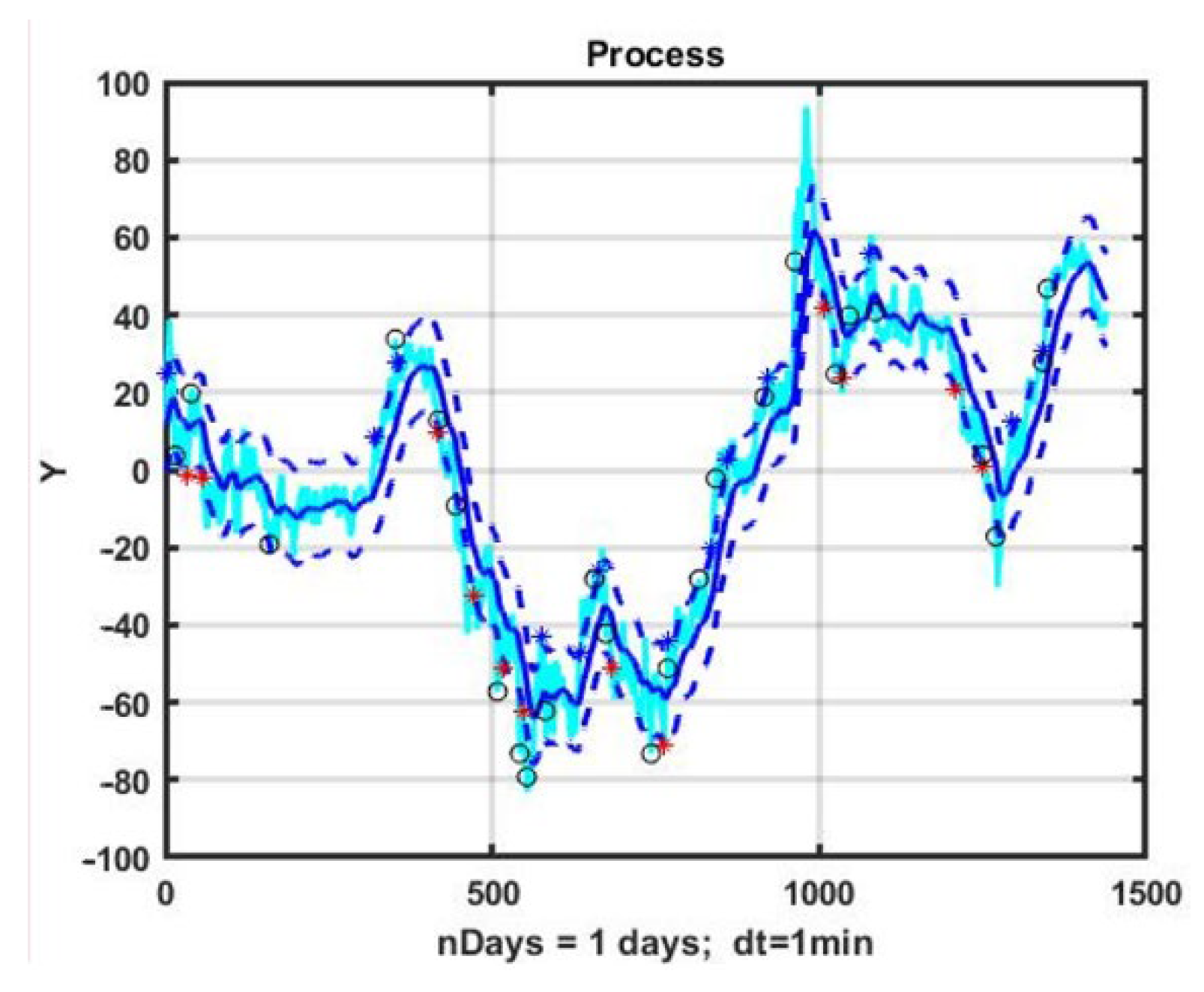
A more flexible control scheme allows for the obtaining of a model in which the upper and lower bounds of the channel are evaluated separately. An example of the implementation of the CSF management strategy for the Euro/Japanese Yen (EURJPY) currency pair on an observation interval of 1440 min counts (one day) is shown in
Figure 1. In this case, the control model was defined by the parameters α = 0.04, B1 = 15, B2 = 15, TP = 15, SL = 15. Blue diamonds indicate opening a position up, red diamonds denote opening a position down, and circles are positions being closed.
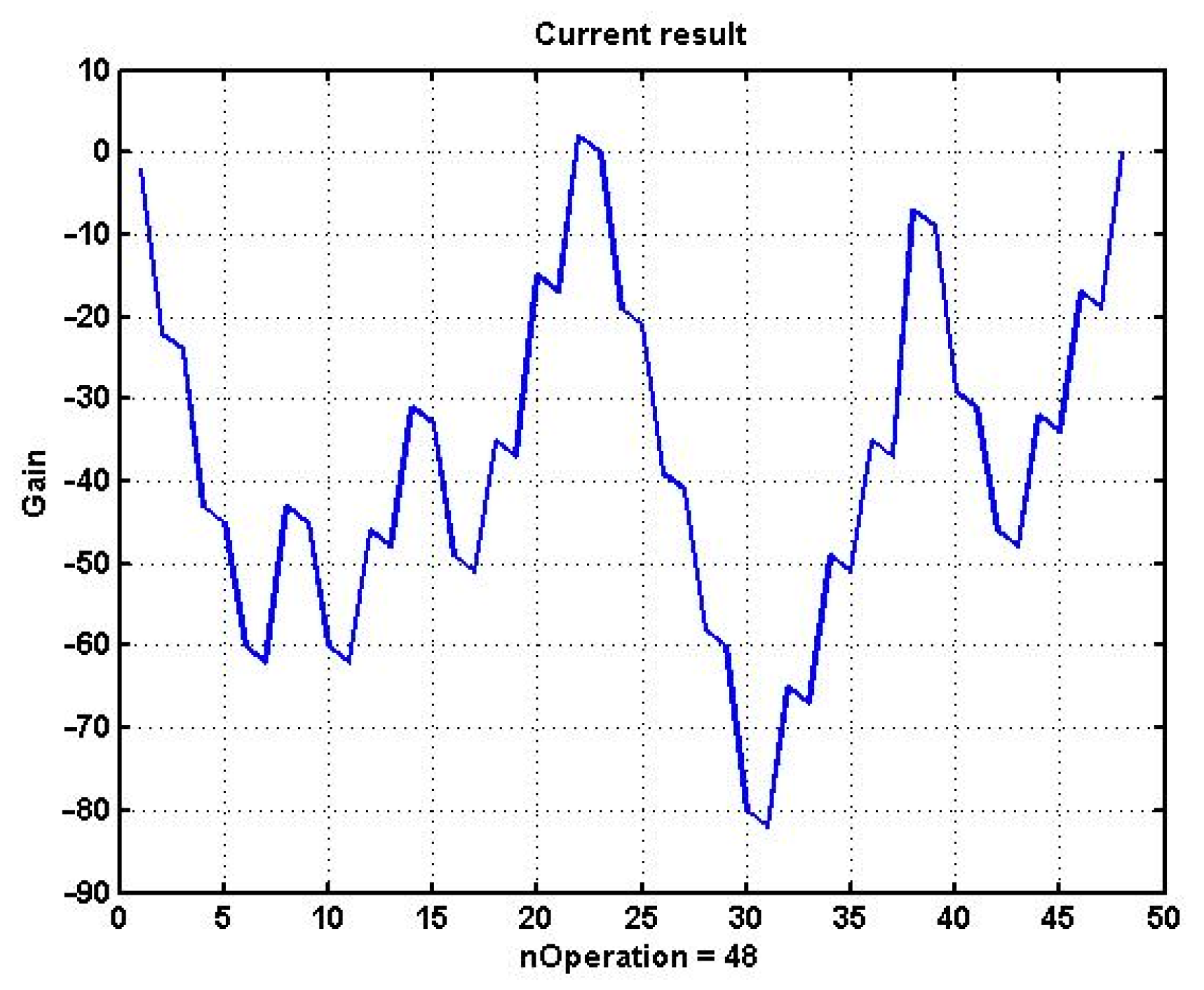
Figure 2 presents management (3) effectiveness fluctuations in utilizing the channel strategy for the selected example. For the parameters that were used for the control model, the result turned out to be close to zero, and most of time during which trading was being carried out, it was negative. Note that in most cases of direct use of the CSF strategy, the result was negative.
Is it possible to achieve profit if there is a reliable forecast of the development of the process? To answer this question, we use bruteforce posterior optimization of the parameters of the management model M = {α, B1, B2, TP, SL}.
For each of the parameters, 15 iterations were carried out, starting from the values of M0 = {0.01, 10, 10, 10, 10}. The values of the iteration step, respectively, were Step = {0.01, 1, 1, 1, 1}.
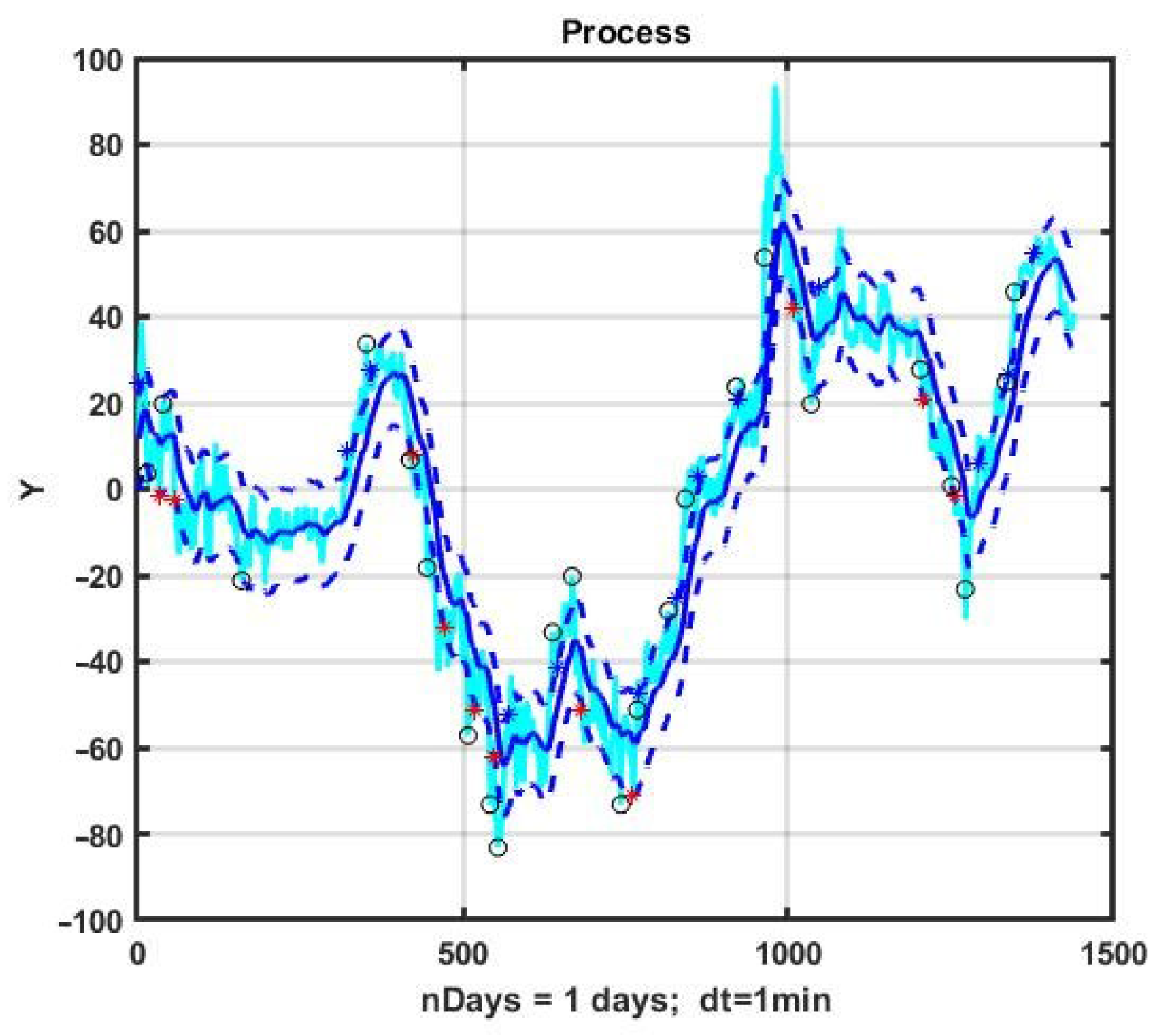
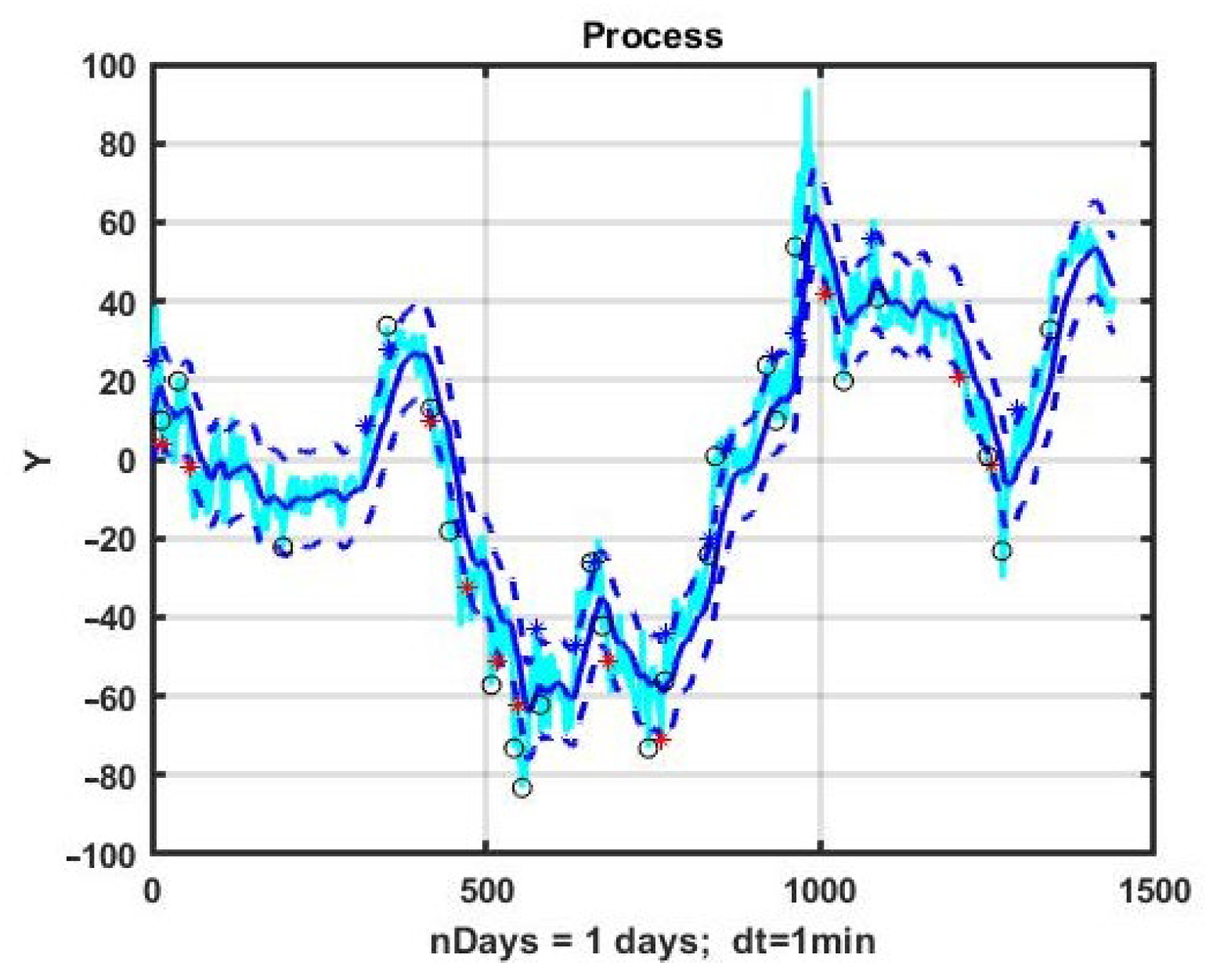
An example of the implementation of the CSF strategy with optimized parameter values α* = 0.05, B1* = 10, B2* = 12, TP* = 18, SL* = 18 at the same observation interval is presented in
Figure 3. Note that this is the same EURJPY price history as in
Figure 1, but the opening and closing moments are different.
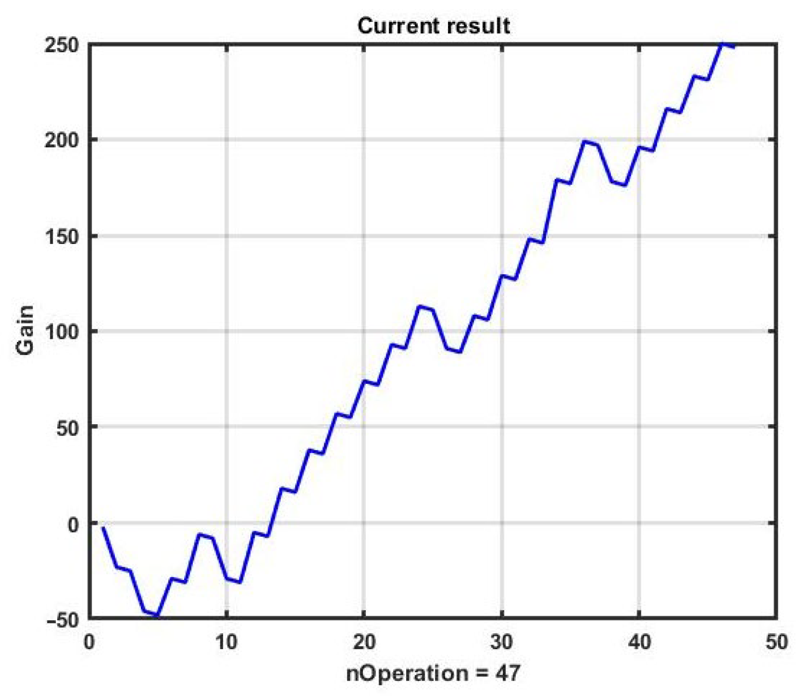
Figure 4 presents the change in performance during the use of CSF with optimized parameters. The management result for the day was G = 248 p.
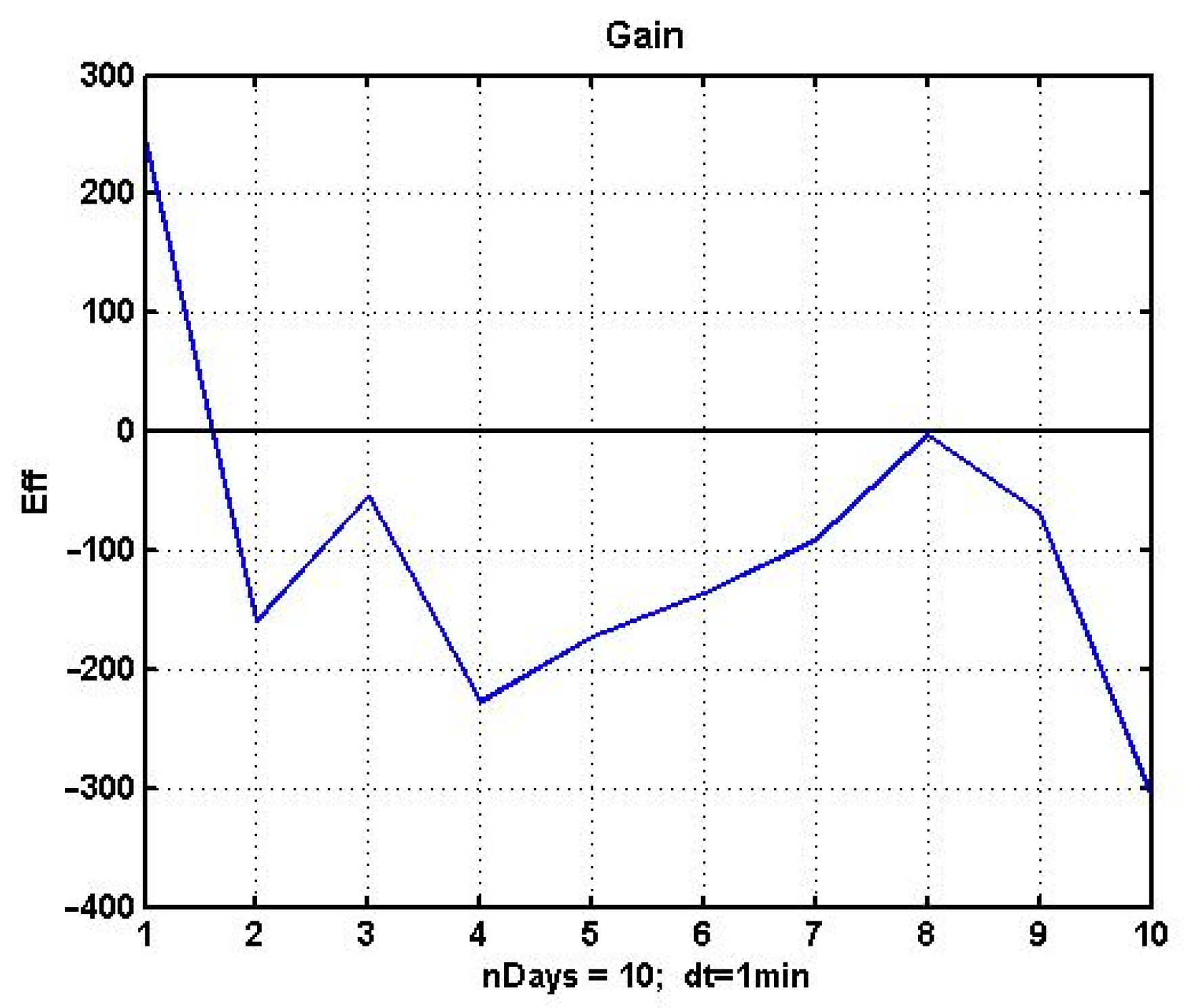
It is not difficult to see that this result is unstable. The results of applying the CSF strategy with the optimal parameters found for the next 10 days of management is shown in
Figure 5. The obtained values completely confirm the instability of the found solution. None of the following nine days of observation produced a profitable result.
Comparing the results presented in
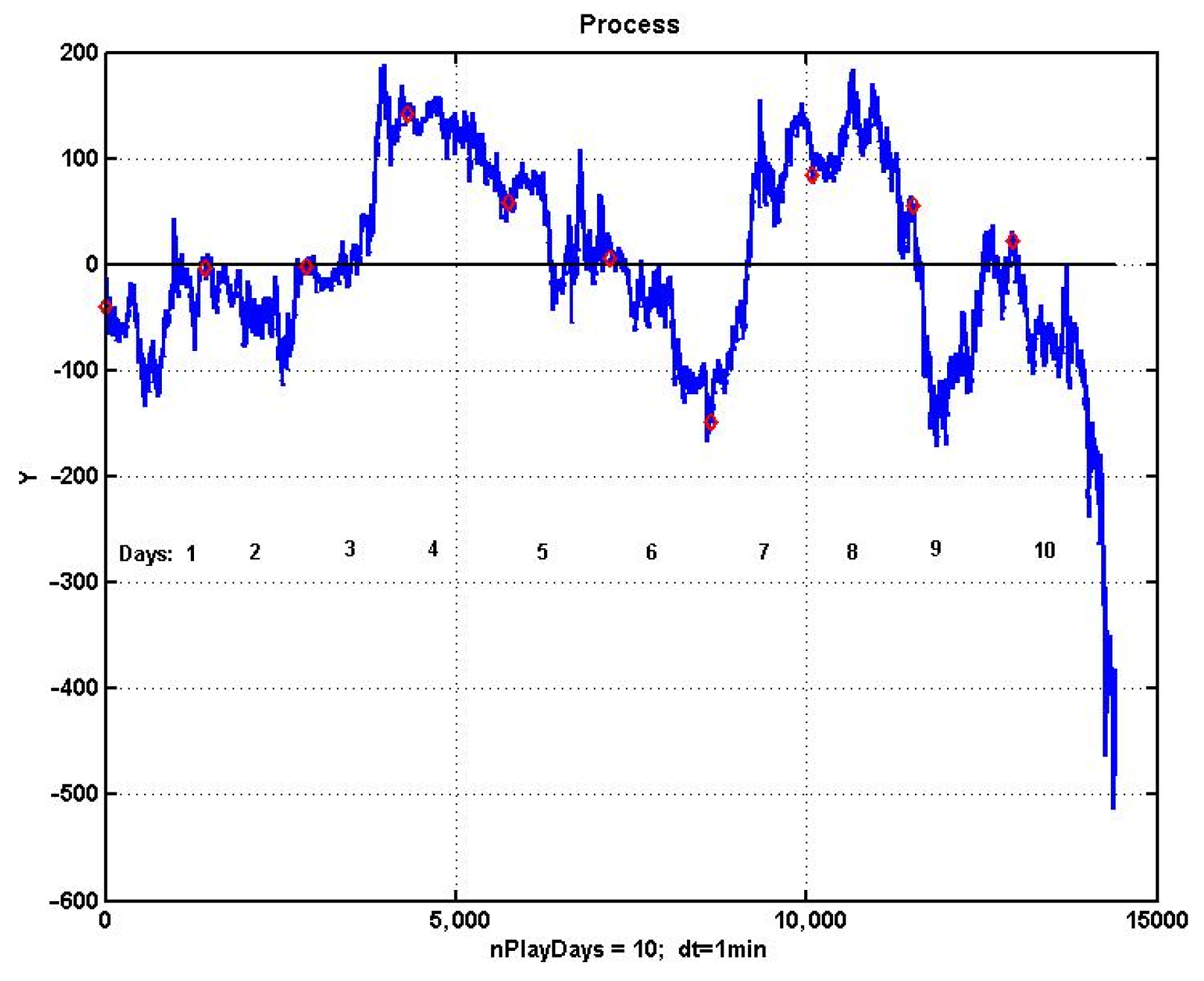
Figure 6 with the dynamics of quotations of a financial instrument at the same observation interval, we can draw another conclusion. The structure of dynamics is more important than the degree of variability of the process. The minimum loss corresponds to the eighth day of observation, the most similar in structure to the first day for which the parameters of the control model were optimized. The worst result corresponds to the last, 10th day, with its strongly pronounced trend.
Thus, in order to preserve, even if not the best, but at least positive result, it is necessary to significantly reduce the size of the time shift at which the optimal parameters are reassessed. This requirement significantly reduces the feasibility of using optimization based on bruteforcing optional parameters. The problem is that the number of calculations shows an exponential increase along with an increase in the number of optimized parameters. It takes about 15 min on a 2.5 GHz 6-core INTEL Core i5 to optimize the model with five parameters by bruteforce on an observation interval of one day. A model with six parameters will take about 1.5 h.
Hence, there is a need to switch to suboptimal computational schemes for sequential optimization, which significantly reduces the calculation time to a level that makes possible real-time sequential data processing.
2.3. Features of Evolutionary Optimization for Chaotic Immersion Environments
In this paper, an algorithm based on the method of evolutionary modeling is proposed as a suboptimal computational scheme for optimizing the management strategy [
38]. Modern computing techniques and applications based on this method can be found in [
39,
40,
41,
42,
43,
44,
45,
46]. Unlike evolutionary modeling, evolutionary optimization of management strategies is not interested in the degree of similarity of the mathematical model to the real data obtained via monitoring the managed object and the parameters of the immersion environment. Its task is to choose a management model that produces the best solution according to (3). Genetic algorithms decrease the volume of computations by about 40% according to estimates given in a number of referenced works.
At the same time, the control strategy itself, as a set of decision rules, can also be modified. The implementation of nonparametric mutations of the management strategy consists in choosing the structure of the model and management rules from the a priori knowledge bank. As a set of decision rules is selected, the list of parameters to be changed, their critical values and ranges of changes are modified. The advantage of this approach is its feasibility. However, at the same time, the arbitrariness of machine choice is limited, and there is no possibility of obtaining radically new strategies that are not provided by the programmer. Any regularization and any set of restrictions can block access to unexpected original solutions.
Moreover, the complete removal of restrictions in the process of random modifications of the structure of strategies leads to a huge number of meaningless decision rules. Waiting for any reasonable solution to appear will take time comparable with real biological evolution. At the same time, the question of artificial generation of management strategies remains open.
Evolutionary technology, like the entire probabilistic-statistical paradigm, is implicitly oriented towards a comfortable hypothesis about the repeatability of experiments in unchanging or slowly changing conditions. The transition to non-stationary, and even chaotic processes, inevitably destroys the optimality of statistical solutions, including those constructed via evolutionary modeling. However, chaos, in general, contains regularizing effects that reduce the degree of total uncertainty. If evolutionary technology can identify, at least not explicitly, and use such hidden patterns, then the task of constructing a winning strategy may be feasible. In addition, using an evolutionary computational scheme will help us answer the question of the fundamental admissibility of particular classes of management strategies.
The paper uses the basic evolutionary modeling algorithm described in [
31]. The return to the original version of this concept is due to the fact that it does not introduce additional restrictions on the mechanism of variability and leaves a wide range of opportunities for its formation. For example, genetic algorithms are focused on the model of bisexual reproduction, which is very important in the implementation of variability in biology. However, for the models under consideration, there is no need to limit the process of variability to the mechanisms of gene exchange. The same can be said about the method of differential evolution. The formation of a new genome, as a mutant vector formed from other parental genomes, also introduces unnecessary restrictions for this case.
In econometric models, one can make any modifications to the structure of genes if they do not contradict common sense and the laws of the market. Therefore, it is reasonable to use the computational scheme of evolutionary optimization, which corresponds to the traditional concept of evolutionary modeling. At the same time, the mechanism of variability is based on the well-known mechanism for extracting a random variable from the range of permissible variations in genome parameters.
2.4. Algorithm of Evolutionary Optimization of the Management Model
Consider a set of ancestor strategies SA = {SA1, …, SANa} with Na elements, each of which is defined by its structure R (the decision-making rule) and a set of corresponding numerical parameters a, i.e., S = {R, a}. The effectiveness of a strategy Eff(s) is assessed via applying it to the time series of observations Y(t), which together form an experimental retrospective dataset. We introduce two nonlinear operators.
Here
is a set of descendant strategies, each of which is created by modifying one of the ancestor strategies,
is the number of descendant strategies in one generation, and
kb > 1 is the multiplication coefficient of strategies. The union of ancestor strategies and descendant strategies is a generation of size
Ng =
Na +
Nd =
Na (1 +
kb):
- 2.
A selection operator that selects the “surviving” strategies from the generation that become the ancestors of the next generation:
Let
be a particular management strategy with the specified parameters, adopted as the basic “parent strategy”. Then evolutionary optimization is reduced to a cyclic execution of an operator sequence:
where arrows denote the sequential order of operators. Since selection is carried out by superiority, the optimality of the final solution is not guaranteed. However, it will be the best of the whole set created during the implementation of evolutionary modeling.
The process of evolutionary optimization is obviously converging to more effective strategies by virtue of its very construction. This is due to the fact that the new generation always includes ancestor strategies in its composition. Consequently, the most effective strategies in principle cannot be discarded by the accepted selection and selection procedure. However, a high convergence rate cannot be expected due to the randomness of the modification process. The convergence rate will be close to the convergence rate of a random search, and depends on the size Ng of the generation being formed. It can be assumed that the convergence rate will be higher if the multiplication coefficient kb is made variable so that the number of descendant strategies Nd depends on the effectiveness of parent strategies, i.e., Nd = k(Eff(Sa)), k > 1. In other words, a more effective ancestor can produce more offspring. However, this statement requires additional verification.
Other regularization methods aimed at increasing the convergence rate of evolutionary optimization are also possible.
2.5. Computational Aspects of the Evolutionary Optimization Algorithm
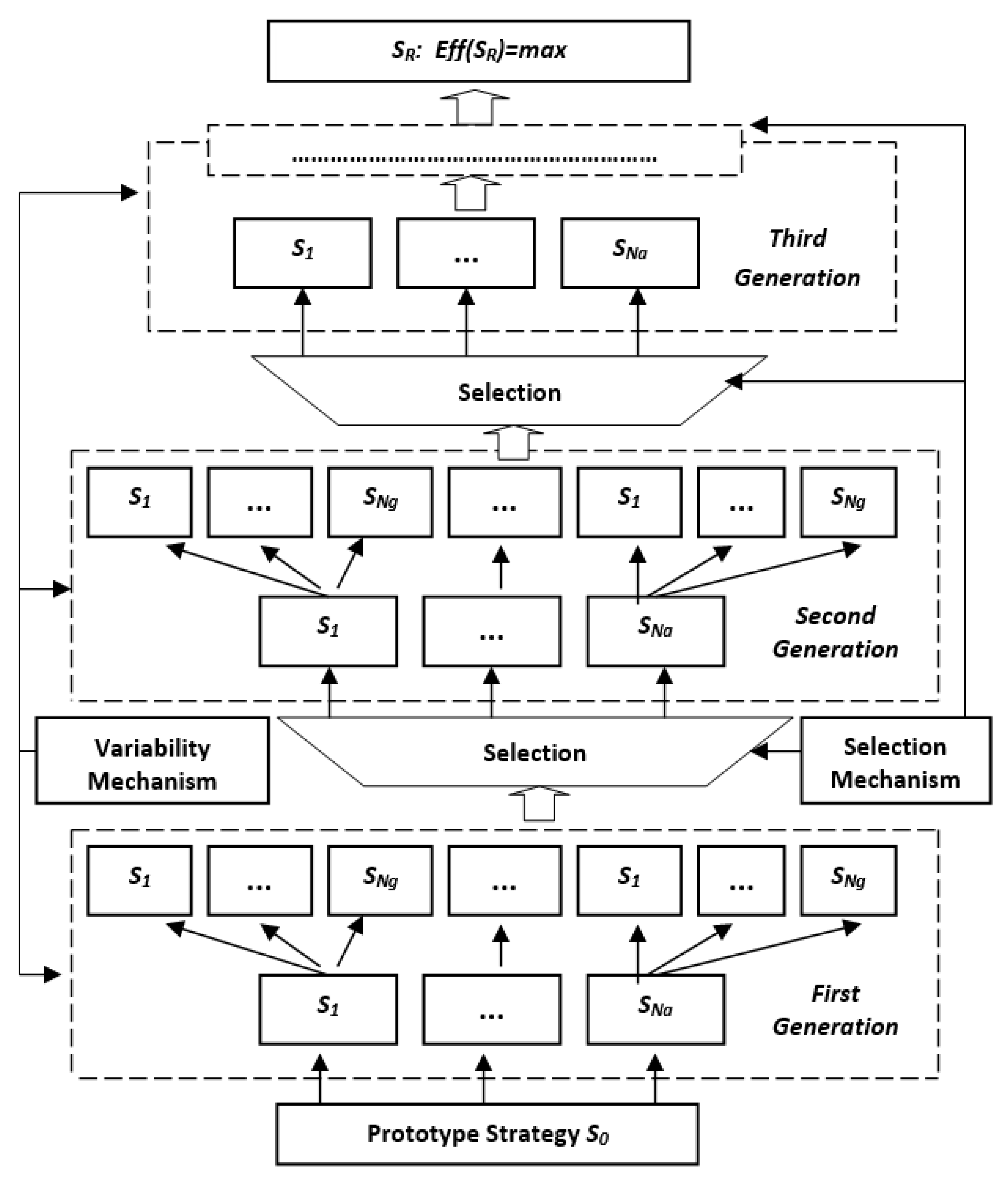
The functional structure of the algorithm of evolutionary optimization of management strategies is shown in
Figure 7. The sequence of evolution is represented by a diagram of a process developing from the bottom up.
Let us consider the presented algorithm. At the preliminary stage, some basic strategy (prototype) is formed. Its structure is chosen either randomly or based on existing a priori experience in asset management. With the help of the variability mechanism, the basic prototype strategy is modified, giving rise to parent strategies.
Then, in accordance with (4), the program loops for the number of successive generations, which are usually called epochs.
At the first step of this loop, the first generation of descendant strategies is formed using the variability generator, which, combined with their parents, form the first generation of strategies SG. Furthermore, each of the first-generation strategies undergoes a testing by being applied to a set of retrospective observations {Y(t), Y(t − Y)}, where T is the size of the validation dataset. The created strategies are ranked by their effectiveness Eff(Si), i = 0, …, Ng and a specified number Na of “surviving” strategies that are allowed for further “reproduction” (modification) are selected. The selected strategies are the parents of a new set of modified descendant strategies and together with them form the second generation.
Furthermore, the cycle is repeated until either a specified number of generations is reached, or, according to some other criterion, for example, when the effectiveness of management does not improve during a given number of epochs.
The variability mechanism used in the program randomly selects changes made to the strategy from the following set of options:
Small single changes. In the strategy undergoing modification, relatively small changes are made to only one parameter (gene) selected by a random draw. The size of the change range depends on the parameter. This one-time change does not usually exceed 10% of the original value. The choice of the parameter is carried out by a random draw, similar to how it happens in the Monte Carlo method.
Small group changes. They are carried out similarly to the previous case, but are made to several gene parameters at once instead. Their amount and their numbers are selected via a random draw.
Strong single mutation or parametric mutation. The gene number is selected via a random draw. Usually, the number of mutations in a generation is small, and the probability of their occurrence does not exceed 2–3%. The size of the change field also depends on the parameter, usually a single mutation can reach 30–50% of the original value.
Strong group changes are similar to the previous case, but are made immediately in several parameters, as in case 2.
Structural (nonparametric) mutations. The parent strategy with some relatively small probability (usually less than 0.01) may undergo nonparametric mutation. In this case, the number of genes in the original genome may change, or, in a more radical case, the management strategy itself may be completely modified. The most rational way in this case consists of randomly choosing a management strategy from an a priori created knowledge base.
It should be expected that such mutations will be quite constructive, since the strategies included in the data bank, to one degree or another, have already been pre-selected by at least the common sense of their developer. For example, there is a transition from a channel strategy to management based on trend analysis, etc. However, this approach limits the evolution to the level of the programmer’s constructive imagination.
A more radical approach consists in stochastic synthesis of new strategies using artificial intelligence technologies. In this case, the evolution program gets out of the strict control of the developer not only at the parametric, but also at the structural level. This approach, in theory, enables the generation of completely new, unexpected solutions. However, in most cases, such mutations will generate ineffective strategies that will be immediately eliminated by the selection mechanism, without generating variants of management strategies in the next generation. In this regard, it may make sense to deliberately preserve such mutations for a given number of epochs and allow them to generate variants of descendants in a mutant zoo.
The selection mechanism, as already noted, ranks a set of strategies according to their effectiveness, and selects among them the best strategies that become the parents of the next generation. It is important to note the principle of incomplete or open solutions, meaning that at each cycle of selection, not the only best option is selected, but a group of strategies is as well. This approach allows us to come to the best solution along a chain consisting of intermediate options other than optimal, which is especially important when searching for effective management strategies in chaotic immersion environments.
3. Results
As an example of the implementation of the evolutionary optimization method, consider the asset management task based on the CSF management strategy. In order to be able to compare with the best solution found by bruteforce, we will consider the same one-day observation interval as in the examples shown in
Figure 1,
Figure 2,
Figure 3 and
Figure 4. As optimization parameters (the genome) we will use M = {α, B1, B2, TP, SL}. From the above optimization example (
Figure 3 and
Figure 4) it follows that the best parameters of the control model are α* = 0.05, B1* = 10, B2* = 12, TP* = 18, SL* = 18.
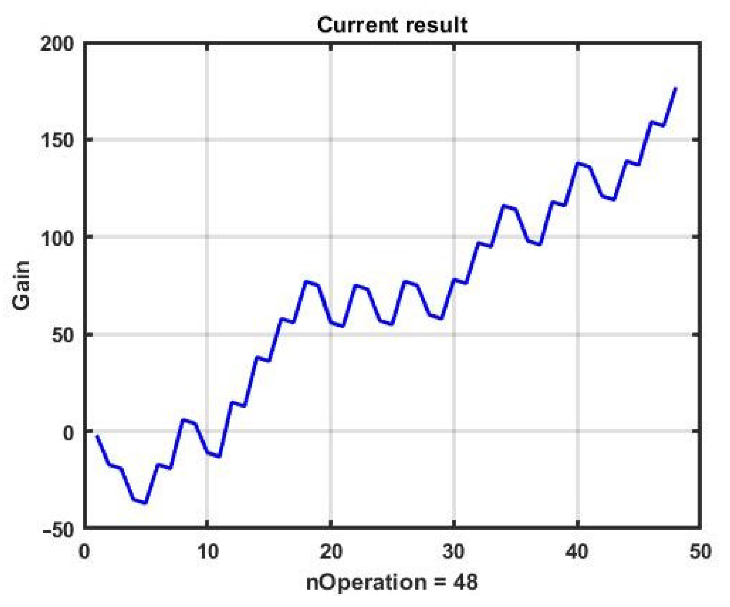
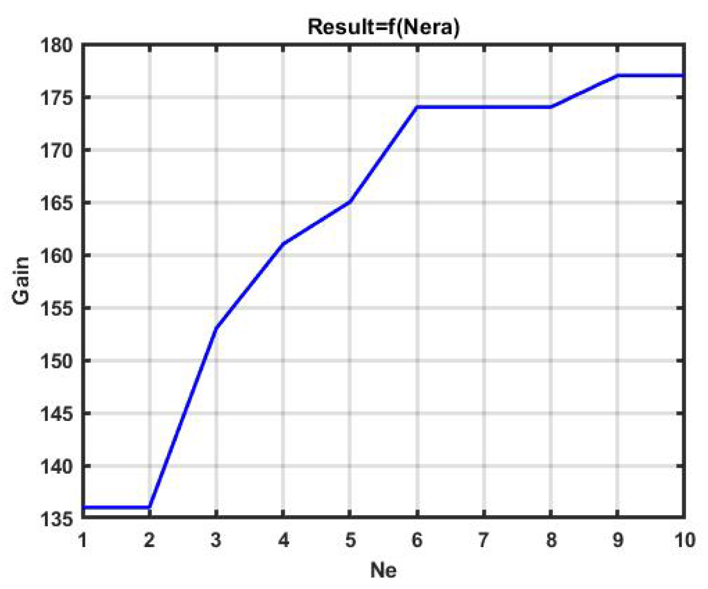
Figure 8 shows an example of CSF implementation with evolutionary optimization of the management model for 10 epochs. The best result was 177 points with the parameters of the model being α* = 0.05, B1* = 12, B2* = 12, TP* = 15.5, SL* = 14.8. The convergence to the found result is shown in
Figure 9.
The dependence of the effectiveness of the CSF strategy during the epoch is shown in
Figure 10.
The plots show that the obtained result, as expected, is inferior to the gain obtained by bruteforce. However, this search only took 0.26 s with the same CPU and with the observation interval the same as in the example with bruteforce optimization, and half of this time was spent on the implementation and output of graphics.
The question arises of how much the quality of management can be improved by increasing the number of epochs.
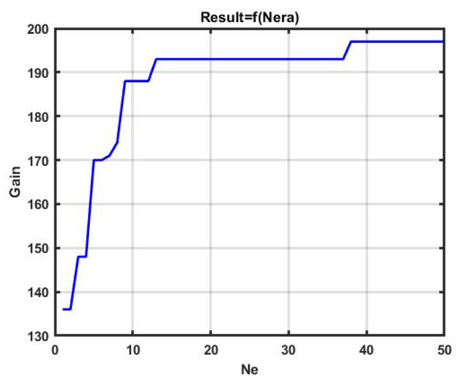
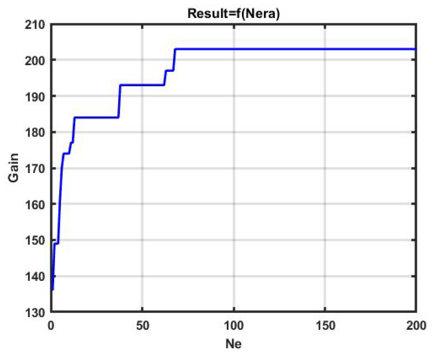
Figure 11 and
Figure 12 show changes in the effectiveness of the best versions of the management model obtained during, 50 and 200 iterations, respectively.
The gain in the above examples reached, 197 p. and 203 p., respectively, did not achieve the effectiveness of bruteforce (248 p). However, the time spent was 0.203 s in the first case, and 0.541 s in the second. A further search for the best option was quite slow, and this can be seen from the section of the horizontal line in
Figure 12, starting from about 70 epochs. Increasing the number of epochs to 500 increased the profit to only 209 p., and spending to 1.17 s.
Note that in the considered examples, a simplified version of the variability operator was used. For example, structural mutation was not used at all. However, even in the proposed case, it becomes possible to conclude that this algorithm is suitable for sequential optimization with new data arriving every 0.5–1 s.
4. Discussion
The chaotic dynamics of quotations, characteristic for electronic capital markets, obstruct the effective use of traditional methods of increasing the stability of management strategies. As shown in the examples in
Figure 5 and
Figure 6, the parameters that are optimal for a given day of observing the dynamics of quotations on the very next day lead to an unpredictable loss. In this regard, the management model should be dynamically corrected as new results of monitoring the market situation become available.
At the same time, the most powerful optimization tool based on bruteforce incurs significant time costs even for modern high-performance processors. This is due to the fact that the time complexity here is described by a power function with an increase in the number of iteration steps, and by an exponential function with an increase in the number of model parameters. As a result, even with a relatively simple model with five to six parameters, the required computational resources exceed the capabilities of modern processors. At the same time, increasing the time interval between successive calculations of the best parameters is unacceptable, given that the dynamics of market assets is absolutely non-inertial and can be discontinuous even within one minute of observation. Due to this, we proposed an optimization of the management model based on evolutionary modeling.
We analyzed the effectiveness of this approach using the example of real data obtained by monitoring the currency exchange market. The results of numerical studies have shown that maximum gain decreased by about 15–20% compared to the result obtained by bruteforcing parameter values. At the same time, the number of operations decreased to such a level that model parameters can be optimized even with a one-second interval of monitoring results.
It is important to note that the potential of evolutionary optimization is by no means exhausted by the version of its implementation considered in the paper. First of all, the above example did not use structural mutations. In essence, we are talking about utilizing qualitatively different strategies, which can give a result that significantly exceeds the mechanistic optimization based on bruteforcing parameter values. Moreover, new opportunities arise, such as artificial intelligence technologies: the computer independently generates management strategies that are not contained in the a priori knowledge base.
The second point related to the advantage of using evolutionary optimization is due to the fact that the drawing of parameter values is carried out on a scale of counts close to continuous. The discreteness is essentially determined only by the mantissa of the bit grid. This means that the conducted adjustment is finer than that obtained with a fixed iteration step. The advantage of fine-tuning is due to the extremely high sensitivity of the management result to variations in the values of the model parameters, which is generally characteristic of a chaotic series of observations.
It should be noted that we used a very simple channel strategy as a demonstration example in this work. This was done in order to ensure the clarity and interpretability of the results. However, in practice, such strategies are not used as is, because in most cases they only lead to loss.
In [
33] it was shown that for almost any variations of the observed dynamic process, profitable solutions exist for this class of strategies. However, their implementation requires fine-tuning, minor deviations from which, as follows from the theory of dynamic chaos, lead to loss. Nevertheless, with a small time shift of observation series relative to the optimization tuning interval, the positive gain on average is preserved. This means that it is fundamentally possible to build a dynamic self-adjusting asset management system. One of the variants of such a solution is considered in this paper.
Other formulations of asset management tasks that also use genetic algorithms for optimization can be seen, for example, in [
47,
48]. At the same time, various algorithms based on random search in some cases lead to completely unexpected and, often, anti-intuitive results [
49,
50].
A development of these studies being focused on constructing a dynamic self-adjusting asset management system with an increased level of resistance to variations in the dynamic and statistical characteristics of observation series implies considering the following points:
the study of potential characteristics of self-adjusting asset management systems for various sets of dynamic properties of observation intervals of chaotic processes;
the development of a knowledge base of management strategies and its application for implementing structural mutations of the management model in the mechanism of variability of the evolutionary optimization algorithm;
the development of randomized synthesis of management strategies using multi-expert data analysis [
51];
the use of composite algorithms combining the capabilities of robustification and adaptation in management decision-making.
the effectiveness of the application of evolutionary optimization in markets and periods that differ in the degree of market efficiency within the Efficient Market Hypothesis (EMH) [
52]. It is supposed that the greatest profit can be made in a highly inefficient market. At the same time various exchange markets all have multifractal structural properties with different levels in the sample and sub-samples that cause inefficiency with different levels in these foreign exchange markets [
30]. Another work reveals that the efficiency of the cryptocurrency markets varies over time, which is consistent with adaptive market hypothesis (AMH) [
53]. The question about the level of current market inefficiency which is acceptable for self-adjusting asset management systems needs to be investigated.
the use of external add-ons that carry information exogenous to technical analysis on expected trends of the considered financial instrument and market mood in general.
The outlined issues constitute the subject of our further research.
