
Chaotic Search-Based Salp Swarm Algorithm for Dealing with System of Nonlinear Equations and Power System Applications

 ,
, 

Abstract
1. Introduction
- (1)
- Presenting a new hybrid algorithm, CSSA, to solve SNLEs.
- (2)
- Introducing a variety of solutions effectively, and preventing CSSA from dropping into the local optima by using CST.
- (3)
- Providing a fine balance between exploration and exploitation trends in CSSA by combining SSA’s exploration and CST’s exploitation abilities.
- (4)
- Applying CST, with a focus on using the infeasible solution, has helped improve performance, avoid the local optima trap, speed up convergence and optimize the search process.
- (5)
- Enhancing the quality of solutions and accelerating convergence to the best results with the hybridization between SSA with CST.
- (6)
- Testing CSSA by using several benchmark problems, as well as two real-world power system applications.
- (7)
- Using the Wilcoxon test to evaluate the significance of the CSSA results.
- (8)
- Displaying that CSSA is competitive and better than other optimization algorithms through statistical analysis and computational results.
2. System of Nonlinear Equations (SNLEs)
Converting the SNLEs into an Optimization Problem
3. Preliminaries
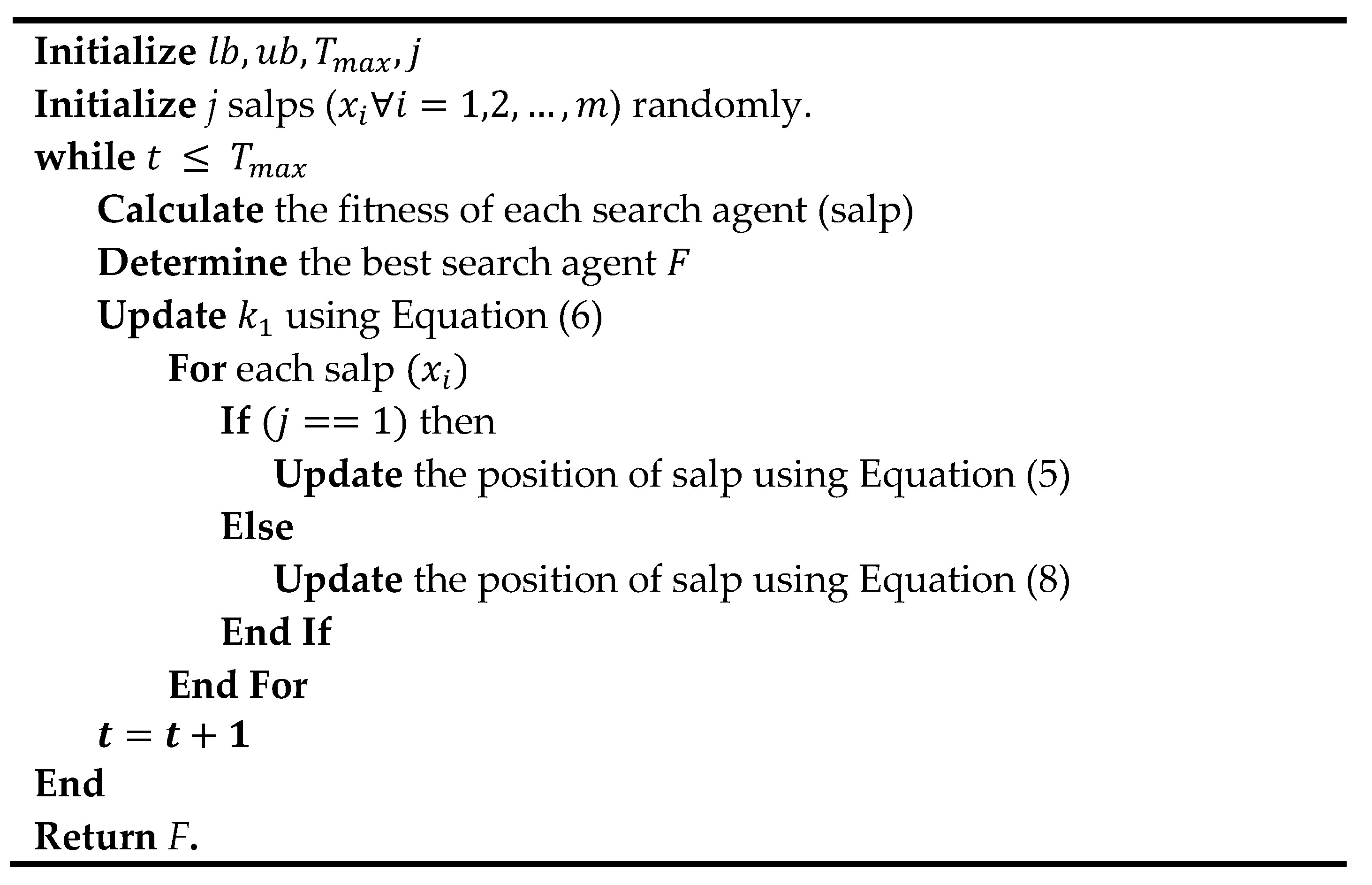
3.1. The Main Characteristics of SSA
3.2. Chaotic Search Technique (CST)
- −
- Chebyshev map: the Chebyshev map [48] is formulated as:
- −
- Singer map: Singer’s chaotic one-dimensional map [49] is defined as the following equation:where
- −
- Sinusoidal map: the following equation is used to create a sinusoidal map [50]:where .
- −
- Piecewise map: a piecewise map [51] can be defined as follows:where and .
- Sine map: the equation for a sine map [52] is as follows:where .
- Circle map: a circle map [53] is described as:where and .
- Intermittency map: the intermittency map [55] can be formulated as:where , and is very close to zero.
- Gauss map/Mouse map: the Gauss map [56] is given by the Gaussian function:where and are real parameters.
- Iterative map: we can formulate the iterative chaotic map [51] as follows:where
- Liebovitch map: we can formulate the Liebovitch chaotic map [48] as follows:where , and .
- Tent map: the tent map [57] is represented as:
4. Chaotic Salp Swarm Algorithm (CSSA)
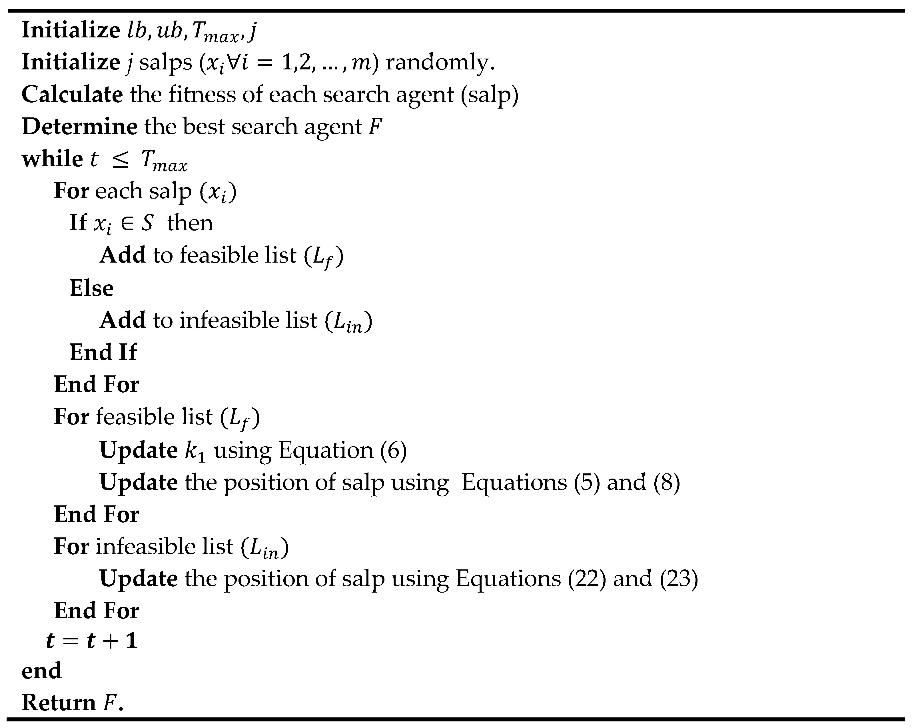
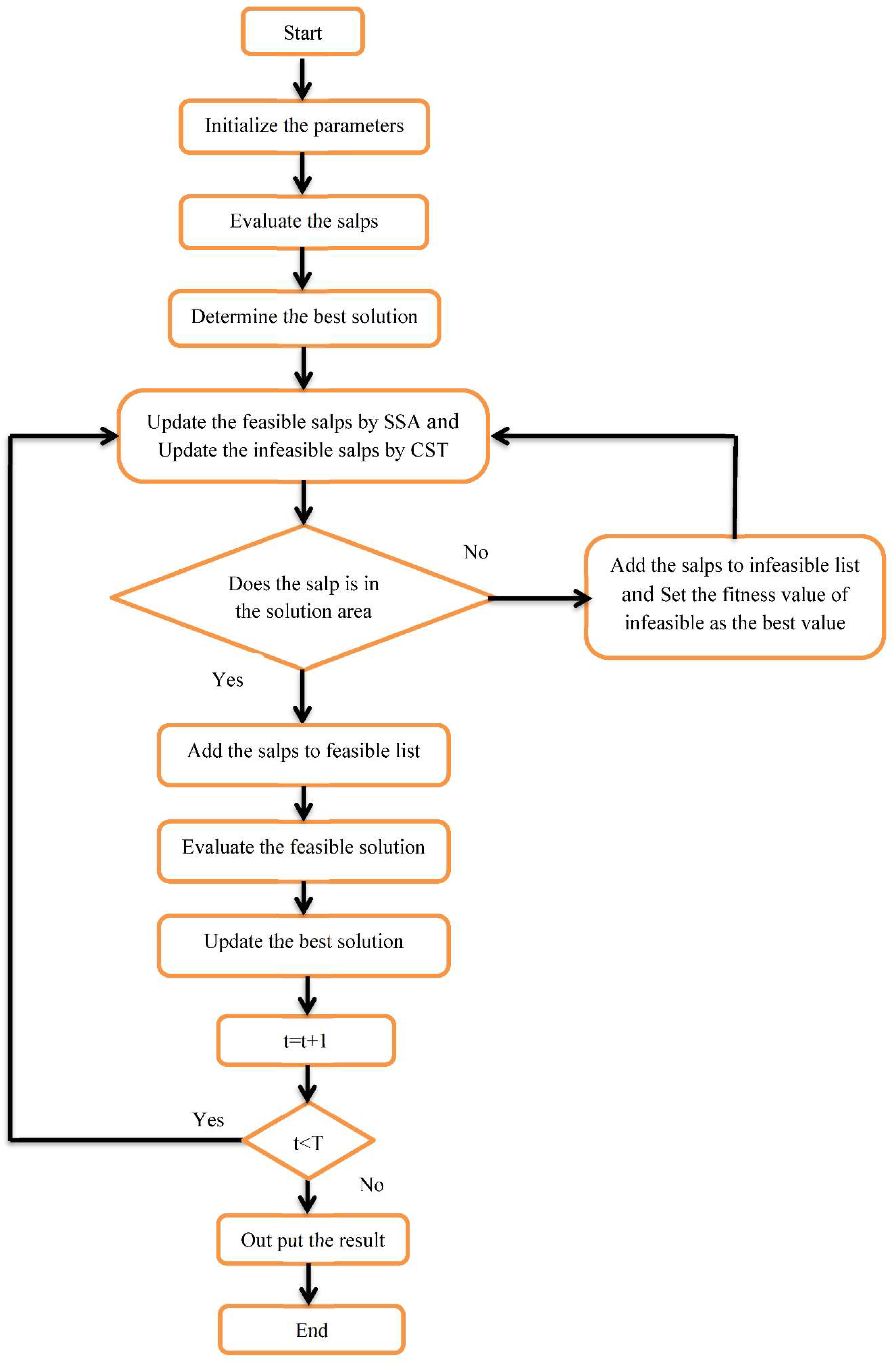
4.1. Steps of the Proposed Algorithm
- Initialize the parameters. Search agents (all salps’ number) are set as , where is the number of salps in the feasible list, and is the number of salps in the infeasible list. The maximum number of iterations are set up to be utilized as the algorithm’s end conditions, using as the iteration counter, lower boundary , upper boundary and the number of variables .
- Initialize the salps’ positions. In the first generation, the salps’ positions are initialized randomly to fulfill the solution space (each variable’s upper and lower limits), using the following equation.where and random numbers dispersed uniformly throughout the range [0, 1] are known as rand.
- Evaluate the salps. According to the needed objective function, every salp is estimated based on the quality of its place, as given in Equation (2), where the best solution (destination) has been documented thus far.
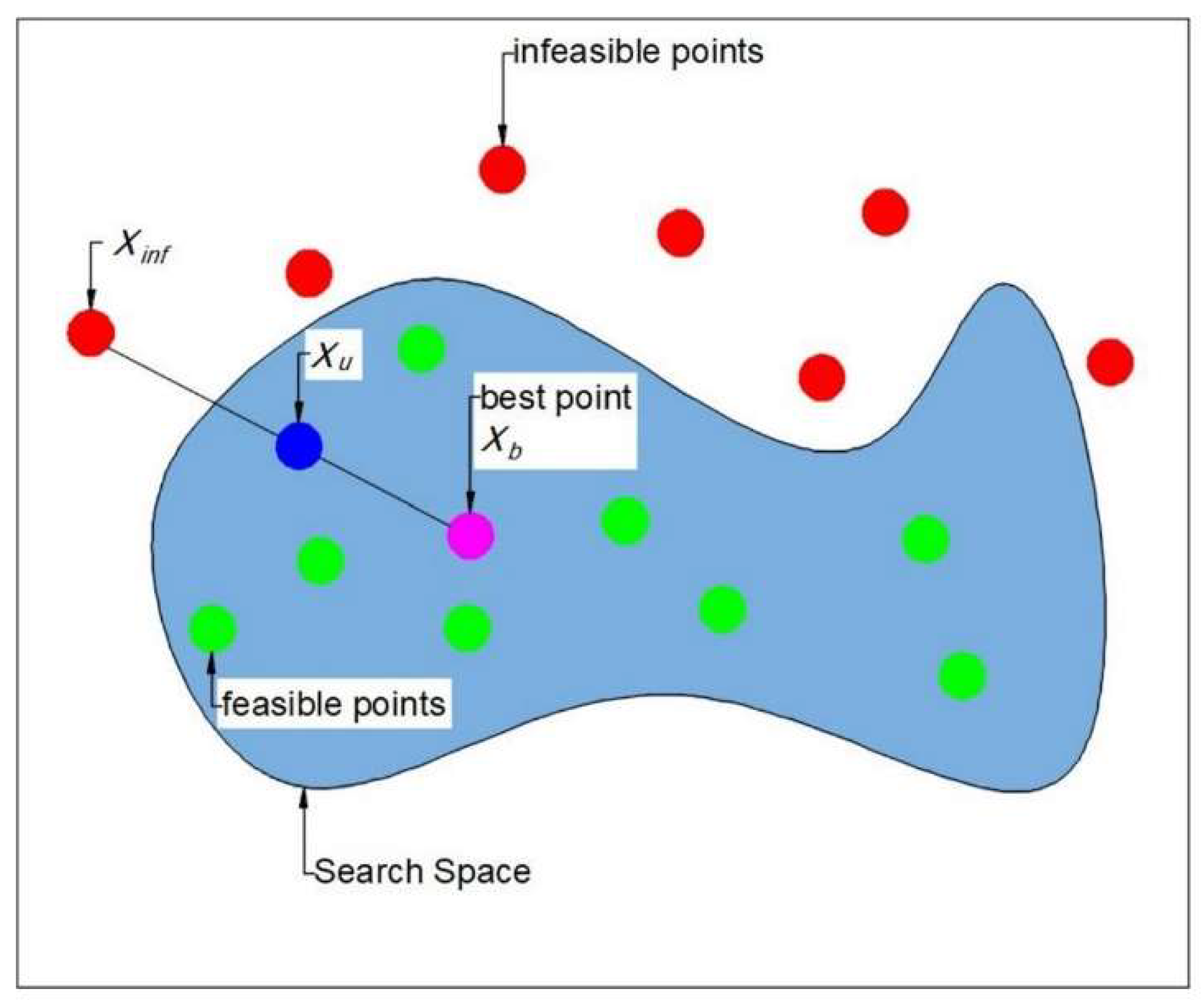
- Update the salps’ positions. Update salps’ positions in the feasible list according to Equation (5) and salps’ positions in the infeasible list with CST according to the following equations:where , is the updated salps’ position, is the position of the infeasible salps and is the best position of feasible salps. Figure 2 shows the updated infeasible solution using the CST.
- Check the feasibility of solutions. Maybe after updating positions, the feasibility of solutions is changed, so we should check the salps’ positions; if the salp exists in the search space, the salp is then considered feasible and is added to the feasible list. Then, we compute the fitness values of the salps. In this case, if the salp is infeasible, it should be added to the infeasible list, and set the fitness value of infeasible as the best value.
- Evaluation of the feasible solutions. Feasible solutions are evaluated.
- Update the best value. Compare the present fitness value with the updated value. If the present value is better than the updated value, then set the present value as the best value. If the updated value is better than the present value, then set the updated value as the best value; then, the corresponding position is the best.
- Termination criteria. Set . If the iterations’ number is greater than the maximum , go to Step 9; otherwise, go to Step 4.
- Output the results. Output the best position and the best fitness value.

4.2. Computational Complexity of the CSSA
5. Numerical Studies
5.1. Testing CSSA on Benchmark Problems
5.2. Wilcoxon Signed Ranks Test (WSRT)
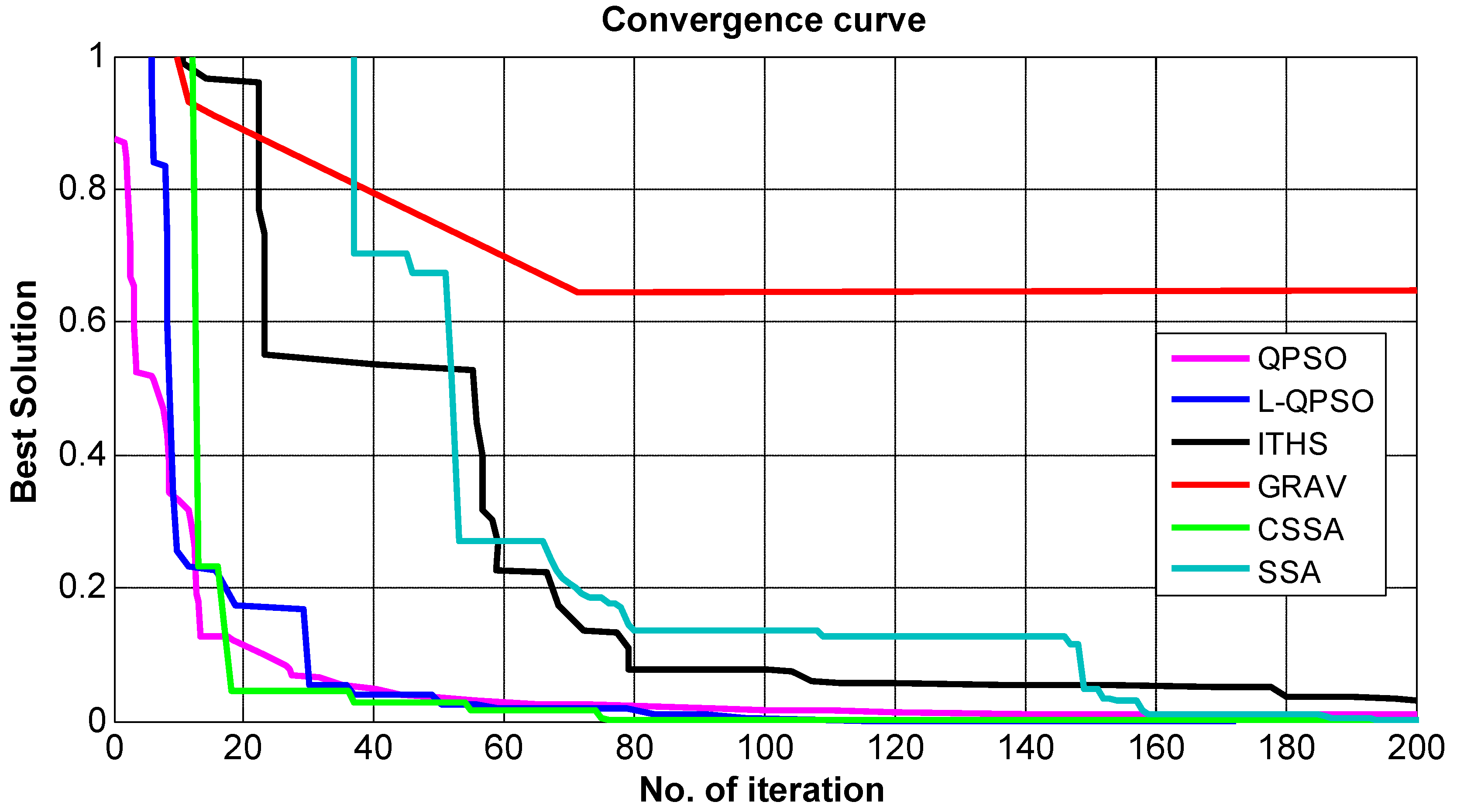
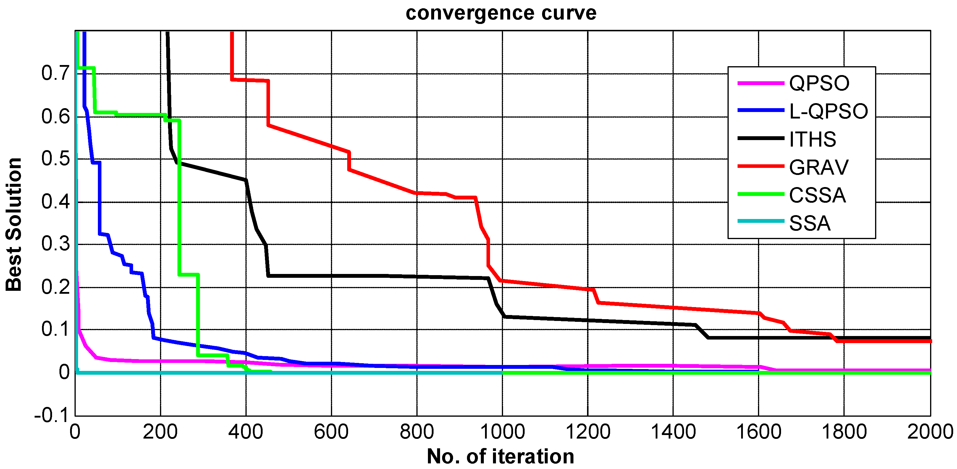
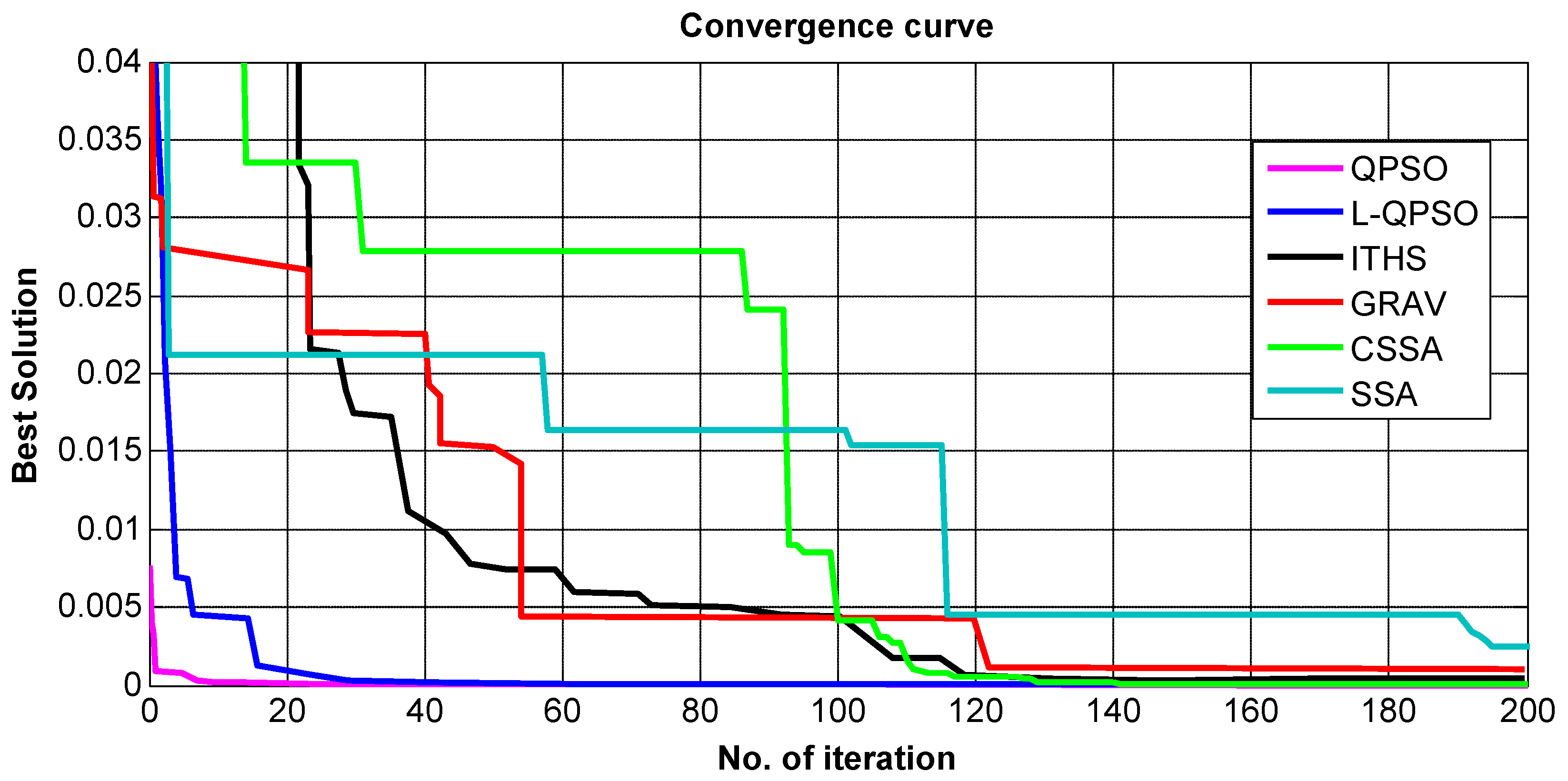
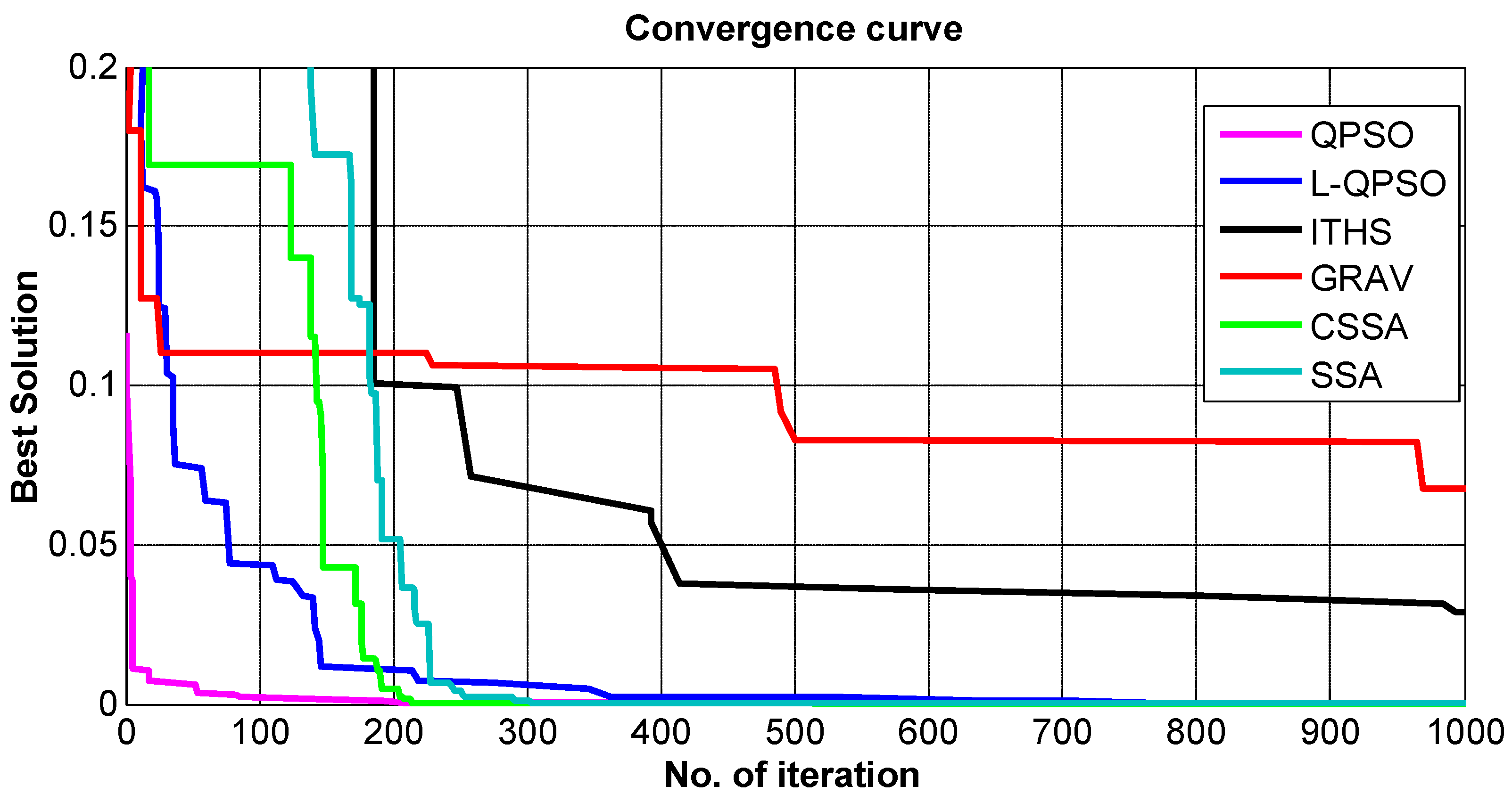
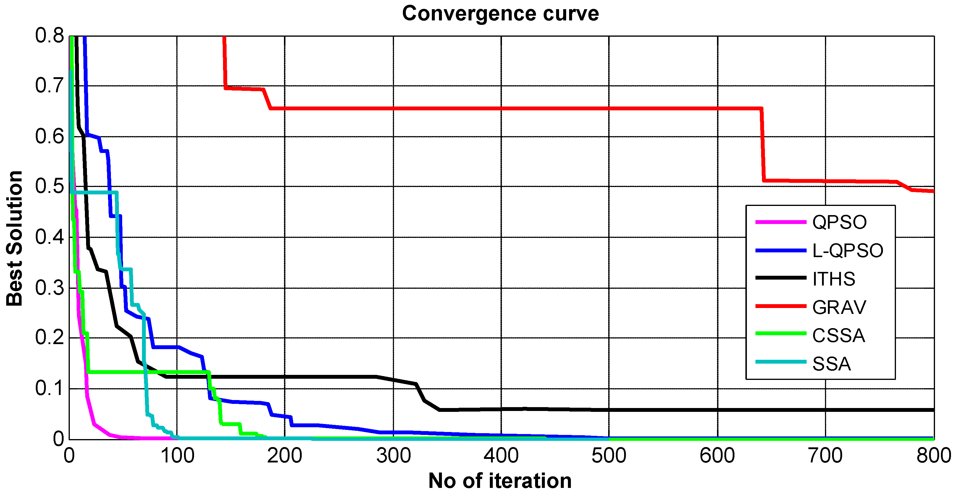
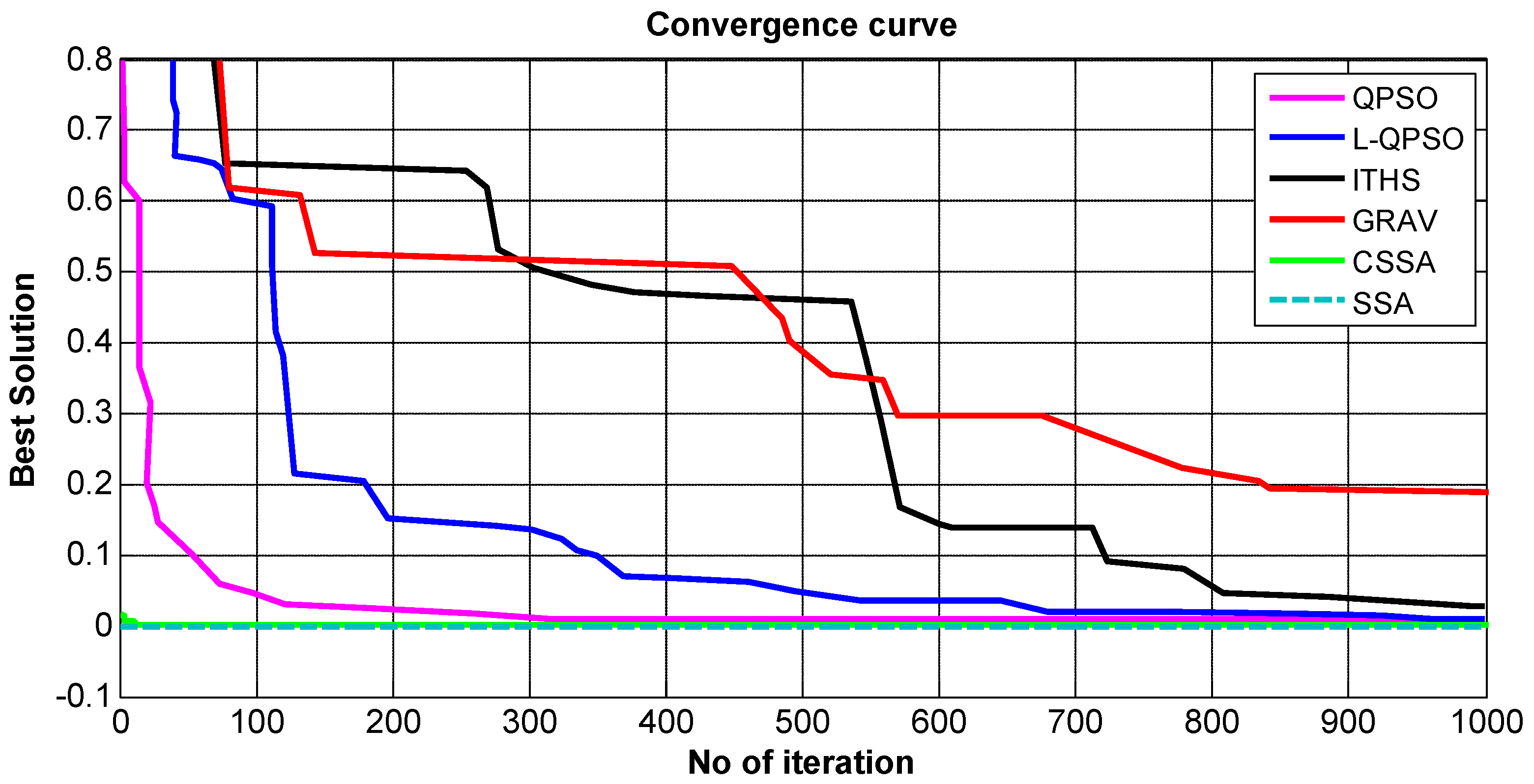
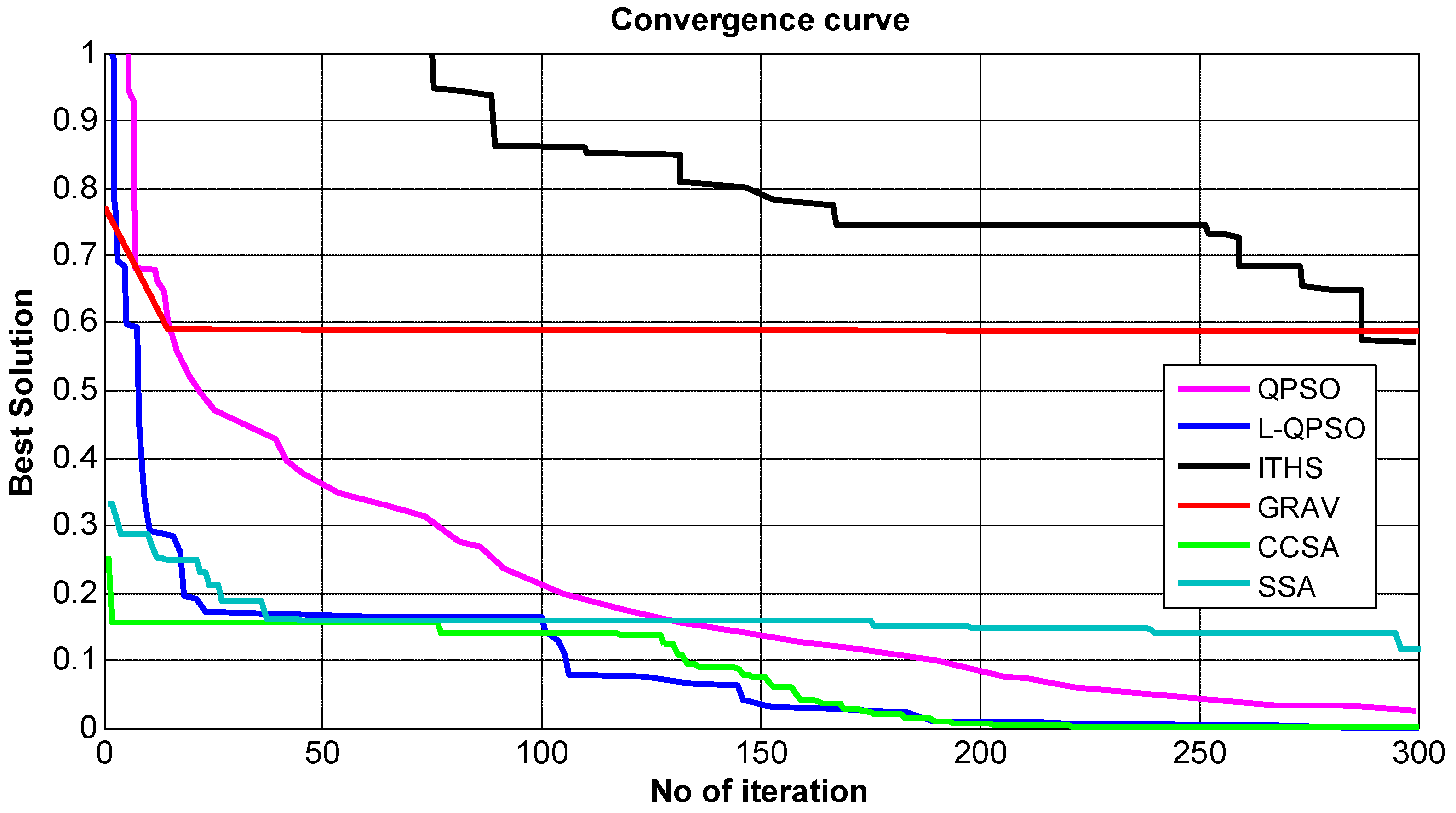
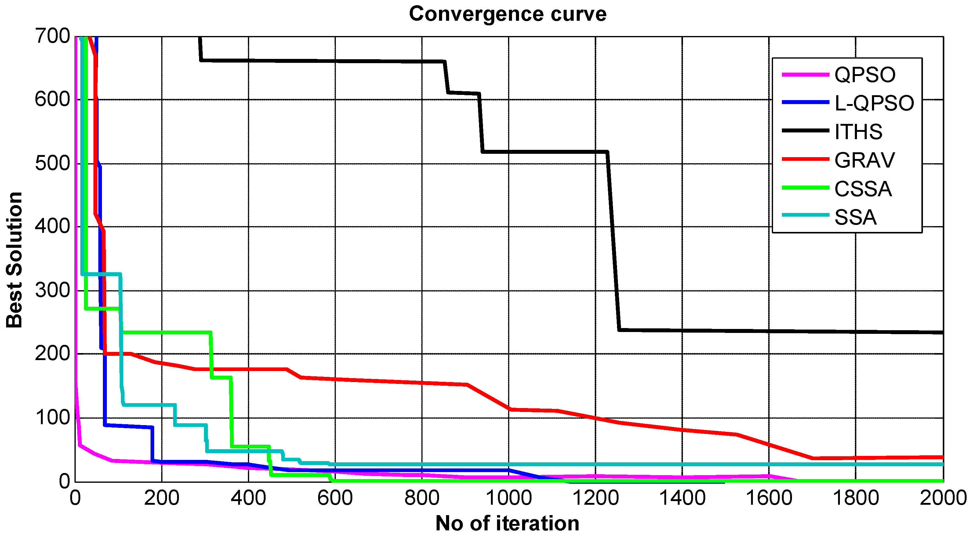
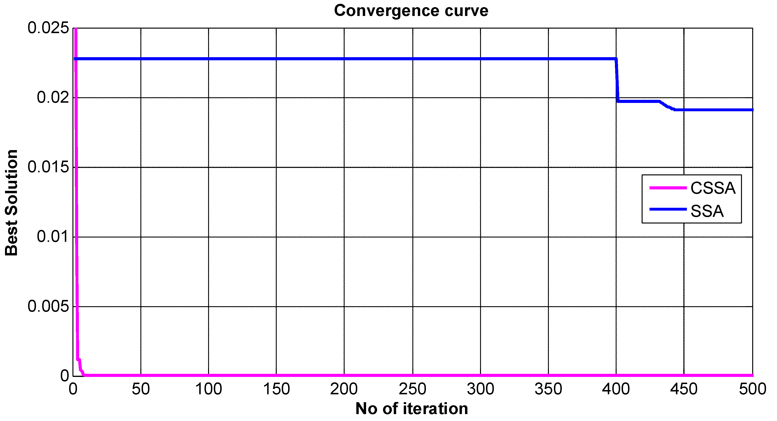
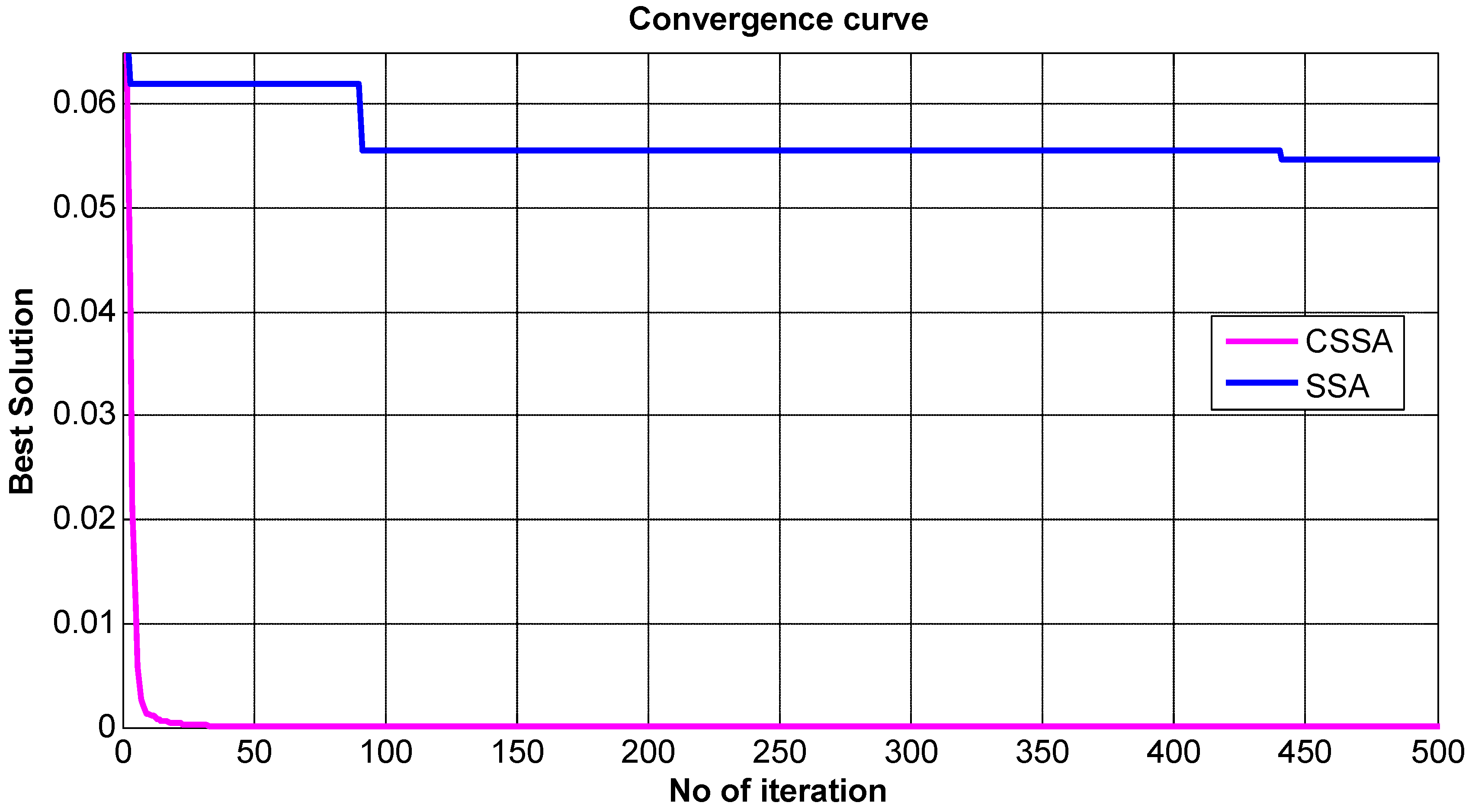
5.3. Convergence Analysis
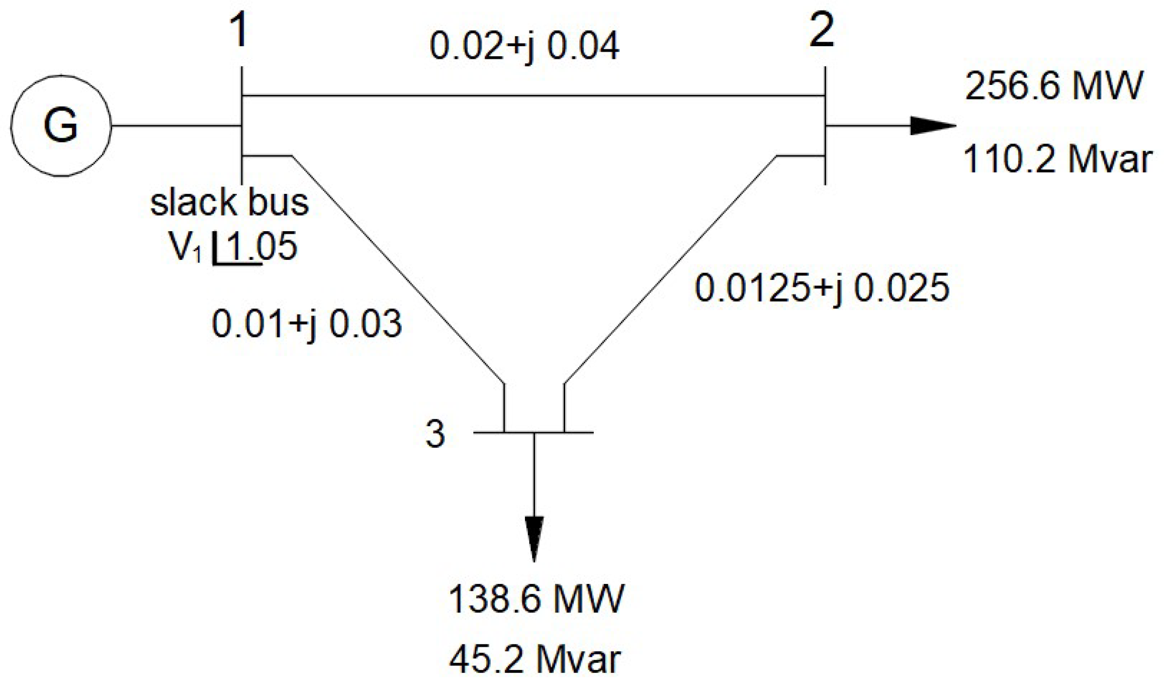
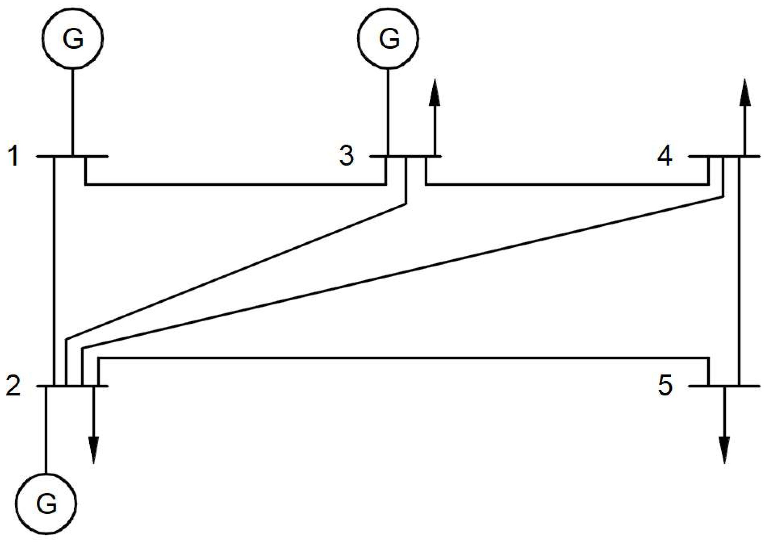
6. Power System Applications
6.1. Formulation of Load Flow Problem
6.1.1. Classification of Buses
- Slack bus
- Generator (PV) bus
- Load (PQ) bus
6.1.2. Node Power Equations
7. Conclusions
- CSSA is simple in application, and it can solve many optimization problems.
- CSSA combines the SSA’s robust global searching capacity with the CST’s substantial chaotic searching ability.
- Only objective function information is used in CSSA; no derivatives or other auxiliary data is used.
- CSSA can transact with the non-continuous, non-differentiable and non-smooth functions that are common in problems of optimization.
- CSSA can give a globally optimal solution because it searches at a set of points, not a single point, unlike traditional techniques.
- The combination between SSA and CST and not ignoring infeasible solutions led to enhancing the efficacy of the search, increasing solution versatility, avoiding the local optima trap, speeding up convergence and optimizing the search process.
- Results have proven the superiority of CSSA over those reported in the literature, as it is significantly better than other comparison methods.
- Statistical results showed that CSSA solutions are more accurate and stable than most other algorithms’ solutions.
- CSSA converges more quickly to the optimal solution in the early iteration.
- A Wilcoxon signed ranks test showed the significance of the CSSA findings.
- By addressing power system applications with CSSA, we can conclude that it is suited for tackling real-world applications that are related to nonlinear system equations.
Author Contributions
Funding
Institutional Review Board Statement
Informed Consent Statement
Data Availability Statement
Conflicts of Interest
References
- Allman, E.S.; Allman, E.S.; Rhodes, J.A. Mathematical Models in Biology: An Introduction; Cambridge University Press: Cambridge, UK, 2004. [Google Scholar]
- Wang, R.; Zhang, Z.; Duan, Y.B. Nonlinear stochastic models of neurons activities. Neurocomputing 2003, 51, 401–411. [Google Scholar] [CrossRef]
- Kerkhoven, T. A Proof of Convergence of Gummel’s Algorithm for Realistic Device Geometries. SIAM J. Numer. Anal. 1986, 23, 1121–1137. [Google Scholar] [CrossRef]
- Bartholomew-Biggs, M. Nonlinear Optimization with Engineering Applications; Springer Science & Business Media: Berlin/Heidelberg, Germany, 2008; Volume 19. [Google Scholar]
- Cuyt, A.; Van der Cruyssen, P. Abstract Padé-approximants for the solution of a sytem of nonlinear equations. Comput. Math. Appl. 1983, 9, 617–624. [Google Scholar] [CrossRef]
- Gragg, W.B.; Stewart, G.W. A stable variant of the secant method for solving nonlinear equations. SIAM J. Numer. Anal. 1976, 13, 889–903. [Google Scholar] [CrossRef]
- Yang, X.S. Firefly algorithms for multimodal optimization. In International Symposium on Stochastic Algorithms; Springer: Berlin/Heidelberg, Germany, 2009; pp. 169–178. [Google Scholar]
- Johari, N.F.; Zain, A.M.; Noorfa, M.H.; Udin, A. Firefly algorithm for optimization problem. In Applied Mechanics and Materials; Trans Tech Publications Ltd.: Bäch, Switzerland, 2013; Volume 421, pp. 512–517. [Google Scholar]
- Dorigo, M.; Stützle, T. The ant colony optimization metaheuristic: Algorithms, applications, and advances. In Handbook of Metaheuristics; Springer: Boston, MA, USA, 2003; pp. 250–285. [Google Scholar]
- Zhao, W.; Wang, L. An effective bacterial foraging optimizer for global optimization. Inf. Sci. 2016, 329, 719–735. [Google Scholar] [CrossRef]
- Bolaji, A.L.A.; Al-Betar, M.A.; Awadallah, M.A.; Khader, A.T.; Abualigah, L.M. A comprehensive review: Krill Herd algorithm (KH) and its applications. Appl. Soft Comput. 2016, 49, 437–446. [Google Scholar] [CrossRef]
- Chu, S.C.; Tsai, P.W.; Pan, J.S. Cat swarm optimization. In Pacific Rim International Conference on Artificial Intelligence; Springer: Berlin/Heidelberg, Germany, 2006; pp. 854–858. [Google Scholar]
- Karaboga, D. An Idea Based on Honey Bee Swarm for Numerical Optimization; Technical Report-tr06; Erciyes University, Engineering Faculty, Computer Engineering Department: Melikgazi/Kayseri, Turkey, 2005; Volume 200, pp. 1–10. [Google Scholar]
- Mirjalili, S. SCA: A sine cosine algorithm for solving optimization problems. Knowl. Based Syst. 2016, 96, 120–133. [Google Scholar] [CrossRef]
- El-Shorbagy, M.A.; Hassanien, A.E. Particle swarm optimization from theory to applications. Int. J. Rough Sets Data Anal. (IJRSDA) 2018, 5, 1–24. [Google Scholar] [CrossRef]
- El-Shorbagy, M.A.; Mousa, A.A. Chaotic particle swarm optimization for imprecise combined economic and emission dispatch problem. Rev. Inf. Eng. Appl. 2017, 4, 20–35. [Google Scholar]
- Abd Allah, A.M.; El-Shorbagy, M.A. Enhanced particle swarm optimization based local search for reactive power compensation problem. Appl. Math. 2017, 3, 9. [Google Scholar]
- Mousa, A.A.; El-Shorbagy, M.A.; Farag, M.A. K-means-clustering based evolutionary algorithm for multi-objective resource allocation problems. Appl. Math. Inf. Sci. 2017, 11, 1681–1692. [Google Scholar] [CrossRef]
- Abdelsalam, A.M.; El-Shorbagy, M.A. Optimization of wind turbines siting in a wind farm using genetic algorithm based local search. Renew. Energy 2018, 123, 748–755. [Google Scholar] [CrossRef]
- Saremi, S.; Mirjalili, S.; Lewis, A. Grasshopper optimisation algorithm: Theory and application. Adv. Eng. Softw. 2017, 105, 30–47. [Google Scholar] [CrossRef]
- Goel, R.; Maini, R. A hybrid of ant colony and firefly algorithms (HAFA) for solving vehicle routing problems. J. Comput. Sci. 2018, 25, 28–37. [Google Scholar] [CrossRef]
- Abd-El-Wahed, W.F.; Mousa, A.A.; El-Shorbagy, M.A. Integrating particle swarm optimization with genetic algorithms for solving nonlinear optimization problems. J. Comput. Appl. Math. 2011, 235, 1446–1453. [Google Scholar] [CrossRef]
- Al Malki, A.; Rizk, M.M.; El-Shorbagy, M.A.; Mousa, A.A. Hybrid genetic algorithm with K-means for clustering problems. Open J. Optim. 2016, 5, 71. [Google Scholar] [CrossRef][Green Version]
- Nasr, S.M.; El-Shorbagy, M.A.; El-Desoky, I.M.; Hendawy, Z.M.; Mousa, A.A. Hybrid genetic algorithm for constrained nonlinear optimization problems. J. Adv. Math. Comput. Sci. 2015, 7, 466–480. [Google Scholar] [CrossRef]
- Wang, J.; Yang, W.; Du, P.; Niu, T. A novel hybrid forecasting system of wind speed based on a newly developed multi-objective sine cosine algorithm. Energy Convers. Manag. 2018, 163, 134–150. [Google Scholar] [CrossRef]
- Skoullis, V.I.; Tassopoulos, I.X.; Beligiannis, G.N. Solving the high school timetabling problem using a hybrid cat swarm optimization based algorithm. Appl. Soft Comput. 2017, 52, 277–289. [Google Scholar] [CrossRef]
- Naderi, E.; Azizivahed, A.; Asrari, A. A step toward cleaner energy production: A water saving-based optimization approach for economic dispatch in modern power systems. Electr. Power Syst. Res. 2022, 204, 107689. [Google Scholar] [CrossRef]
- Wu, J.; Cui, Z.; Liu, J. Using hybrid social emotional optimization algorithm with metropolis rule to solve nonlinear equations. In Proceedings of the IEEE 10th International Conference on Cognitive Informatics and Cognitive Computing (ICCI-CC’11), Banff, AB, Canada, 18–20 August 2011; IEEE: Piscataway, NJ, USA, 2011; pp. 405–411. [Google Scholar]
- Jaberipour, M.; Khorram, E.; Karimi, B. Particle swarm algorithm for solving systems of nonlinear equations. Comput. Math. Appl. 2011, 62, 566–576. [Google Scholar] [CrossRef]
- Wu, Z.; Kang, L. A fast and elitist parallel evolutionary algorithm for solving systems of non-linear equations. In Proceedings of the 2003 Congress on Evolutionary Computation, Canberra, ACT, Australia, 8–12 December 2003; IEEE: Piscataway, NJ, USA, 2003. CEC’03. Volume 2, pp. 1026–1028. [Google Scholar]
- Dai, J.; Wu, G.; Wu, Y.; Zhu, G. Helicopter trim research based on hybrid genetic algorithm. In Proceedings of the 2008 7th World Congress on Intelligent Control and Automation, Chongqing, China, 25–27 June 2008; IEEE: Piscataway, NJ, USA, 2008; pp. 2007–2011. [Google Scholar]
- Mo, Y.; Liu, H.; Wang, Q. Conjugate direction particle swarm optimization solving systems of nonlinear equations. Comput. Math. Appl. 2009, 57, 1877–1882. [Google Scholar] [CrossRef]
- Dos Santos Coelho, L.; Mariani, V.C. Use of chaotic sequences in a biologically inspired algorithm for engineering design optimization. Expert Syst. Appl. 2008, 34, 1905–1913. [Google Scholar] [CrossRef]
- Zhang, L.; Zhang, C. Hopf bifurcation analysis of some hyperchaotic systems with time-delay controllers. Kybernetika 2008, 44, 35–42. [Google Scholar]
- Yang, D.; Li, G.; Cheng, G. On the efficiency of chaos optimization algorithms for global optimization. Chaos Solitons Fractals 2007, 34, 1366–1375. [Google Scholar] [CrossRef]
- Abdullah, A.H.; Enayatifar, R.; Lee, M. A hybrid genetic algorithm and chaotic function model for image encryption. AEU-Int. J. Electron. Commun. 2012, 66, 806–816. [Google Scholar] [CrossRef]
- Jiang, B.L.W. Optimizing complex functions by chaos search. Cybern. Syst. 1998, 29, 409–419. [Google Scholar] [CrossRef]
- Saremi, S.; Mirjalili, S.; Lewis, A. Biogeography-based optimisation with chaos. Neural Comput. Appl. 2014, 25, 1077–1097. [Google Scholar] [CrossRef]
- Singh, H.K.; Alam, K.; Ray, T. Use of infeasible solutions during constrained evolutionary search: A short survey. In Proceedings of the Australasian Conference on Artificial Life and Computational Intelligence, Geelong, Australia, 31 January–2 February 2016; Springer: Cham, Switzerland, 2016; pp. 193–205. [Google Scholar]
- Mirjalili, S.; Gandomi, A.H.; Mirjalili, S.Z.; Saremi, S.; Faris, H.; Mirjalili, S.M. Salp Swarm Algorithm: A bio-inspired optimizer for engineering design problems. Adv. Eng. Softw. 2017, 114, 163–191. [Google Scholar] [CrossRef]
- Nie, P.Y. An SQP approach with line search for a system of nonlinear equations. Math. Comput. Model. 2006, 43, 368–373. [Google Scholar] [CrossRef]
- Nie, P.Y. A null space method for solving system of equations. Appl. Math. Comput. 2004, 149, 215–226. [Google Scholar] [CrossRef]
- Grosan, C.; Abraham, A. A new approach for solving nonlinear equations systems. IEEE Trans. Syst. Man Cybern. Part A Syst. Hum. 2008, 38, 698–714. [Google Scholar] [CrossRef]
- Chen, L.; McPhee, J.; Yeh, W.W.G. A diversified multiobjective GA for optimizing reservoir rule curves. Adv. Water Resour. 2007, 30, 1082–1093. [Google Scholar] [CrossRef]
- Pourrajabian, A.; Ebrahimi, R.; Mirzaei, M.; Shams, M. Applying genetic algorithms for solving nonlinear algebraic equations. Appl. Math. Comput. 2013, 219, 11483–11494. [Google Scholar] [CrossRef]
- Skiadas, C.H.; Skiadas, C. (Eds.) Handbook of Applications of Chaos Theory; CRC Press: Boca Raton, FL, USA, 2017. [Google Scholar]
- Kaveh, A. Advances in Metaheuristic Algorithms for Optimal Design of Structures; Springer International Publishing: Cham, Switzerland, 2014; pp. 9–40. [Google Scholar]
- Tavazoei, M.S.; Haeri, M. Comparison of different one-dimensional maps as chaotic search pattern in chaos optimization algorithms. Appl. Math. Comput. 2007, 187, 1076–1085. [Google Scholar] [CrossRef]
- Peitgen, H.O.; Jürgens, H.; Saupe, D. Chaos and Fractals; Springer: New York, NY, USA, 1992. [Google Scholar]
- Li, Y.; Deng, S.; Xiao, D. A novel Hash algorithm construction based on chaotic neural network. Neural Comput. Appl. 2011, 20, 133–141. [Google Scholar] [CrossRef]
- May, R.M. Simple mathematical models with very complicated dynamics. In Theory Chaotic Attractors; Springer: New York, NY, USA, 2004; pp. 85–93. [Google Scholar]
- Devaney, R.L.; Wiggins, S. A review of: “An introduction to chaotic dynamical systems” (benjamin/cummings, menlo park 1987, 1986). Transp. Theory Stat. Phys. 1987, 16, 1177–1180. [Google Scholar] [CrossRef]
- Hilborn, R.C. Chaos and Nonlinear Dynamics: An Introduction for Scientists and Engineers; Oxford University Press on Demand: Oxford, UK, 2000. [Google Scholar]
- Arora, J.S.; Elwakeil, O.A.; Chahande, A.I.; Hsieh, C.C. Global optimization methods for engineering applications: A review. Struct. Optim. 1995, 9, 137–159. [Google Scholar] [CrossRef]
- Erramilli, A.; Singh, R.P.; Pruthi, P. Modeling Packet Traffic with Chaotic Maps; KTH: Stockholm, Sweden, 1994. [Google Scholar]
- He, D.; He, C.; Jiang, L.G.; Zhu, H.W.; Hu, G.R. Chaotic characteristics of a one-dimensional iterative map with infinite collapses. IEEE Trans. Circuits Syst. I Fundam. Theory Appl. 2001, 48, 900–906. [Google Scholar]
- Ott, E. Chaos in Dynamical Systems; Cambridge University Press: Cambridge, UK, 2002. [Google Scholar]
- El-Shorbagy, M.A.; Mousa, A.A.; Nasr, S.M. A chaos-based evolutionary algorithm for general nonlinear programming problems. Chaos Solitons Fractals 2016, 85, 8–21. [Google Scholar] [CrossRef]
- Rashedi, E.; Nezamabadi-Pour, H.; Saryazdi, S. GSA: A gravitational search algorithm. Inf. Sci. 2009, 179, 2232–2248. [Google Scholar] [CrossRef]
- Sun, J.; Feng, B.; Xu, W. Particle swarm optimization with particles having quantum behavior. In Proceedings of the 2004 Congress on Evolutionary Computation, Portland, OR, USA, 19–23 June 2004; IEEE Cat. No. 04TH8753. IEEE: Piscataway, NJ, USA, 2004; Volume 1, pp. 325–331. [Google Scholar]
- Sun, J.; Xu, W.; Feng, B. Adaptive parameter control for quantum-behaved particle swarm optimization on individual level. In Proceedings of the 2005 IEEE International Conference on Systems, Man and Cybernetics, Waikoloa, HI, USA, 12 October 2005; IEEE: Piscataway, NJ, USA, 2005; Volume 4, pp. 3049–3054. [Google Scholar]
- Yadav, P.; Kumar, R.; Panda, S.K.; Chang, C.S. An intelligent tuned harmony search algorithm for optimisation. Inf. Sci. 2012, 196, 47–72. [Google Scholar] [CrossRef]
- Turgut, O.E.; Turgut, M.S.; Coban, M.T. Chaotic quantum behaved particle swarm optimization algorithm for solving nonlinear system of equations. Comput. Math. Appl. 2014, 68, 508–530. [Google Scholar] [CrossRef]
- Floudas, C.A.; Pardalos, P.M.; Adjiman, C.; Esposito, W.R.; Gümüs, Z.H.; Harding, S.T.; Klepeis, J.L.; Meyer, C.A.; Schweiger, C.A. Handbook of Test Problems in Local and Global Optimization; Springer Science & Business Media: Berlin/Heidelberg, Germany, 2013; Volume 33. [Google Scholar]
- e Oliveira, H.A., Jr.; Petraglia, A. Solving nonlinear systems of functional equations with fuzzy adaptive simulated annealing. Appl. Soft Comput. 2013, 13, 4349–4357. [Google Scholar] [CrossRef]
- Abdollahi, M.; Isazadeh, A.; Abdollahi, D. Imperialist competitive algorithm for solving systems of nonlinear equations. Comput. Math. Appl. 2013, 65, 1894–1908. [Google Scholar] [CrossRef]
- Wang, C.; Luo, R.; Wu, K.; Han, B. A new filled function method for an unconstrained nonlinear equation. J. Comput. Appl. Math. 2011, 235, 1689–1699. [Google Scholar] [CrossRef]
- Luo, Y.Z.; Tang, G.J.; Zhou, L.N. Hybrid approach for solving systems of nonlinear equations using chaos optimization and quasi-Newton method. Appl. Soft Comput. 2008, 8, 1068–1073. [Google Scholar] [CrossRef]
- Mageshvaran, R.; Raglend, I.J.; Yuvaraj, V.; Rizwankhan, P.G.; Vijayakumar, T. Implementation of non-traditional optimization techniques (PSO, CPSO, HDE) for the optimal load flow solution. In Proceedings of the TENCON 2008 IEEE Region 10 Conference, Hyderabad, India, 19–21 November 2008; IEEE: Piscataway, NJ, USA, 2018; pp. 1–6. [Google Scholar]
- Saadat, H. Power System Analysis, 2nd ed.; McGraw-Hill Higher Education: Singapore, 2009. [Google Scholar]
- Milano, F. Continuous Newton’s method for power flow analysis. IEEE Trans. Power Syst. 2008, 24, 50–57. [Google Scholar] [CrossRef]
- Rizk-Allah, R.M. A quantum-based sine cosine algorithm for solving general systems of nonlinear equations. Artif. Intell. Rev. 2021, 54, 3939–3990. [Google Scholar] [CrossRef]


| CSSA | SSA | L-QPSO | QPSO | ITHS | GRAV | |
|---|---|---|---|---|---|---|
| y1 | 0.995903811683832 | 0.992951171841475 | 1.418227087330760 | 1.000144199216134 | 0.999999983928838 | 0.916566028481882 |
| y2 | 0.995903811683831 | 0.992980846443041 | 0.916354582533385 | 1.000120111355508 | 0.999999984261559 | 0.916262407670433 |
| y3 | 0.995903811683832 | 0.993004941523888 | 0.916354582533385 | 1.000131686228283 | 0.999999984646038 | 0.916981249858047 |
| y4 | 0.995903811683831 | 0.992853011911152 | 0.916354582533385 | 1.000129832805469 | 0.999999984062309 | 0.916141646585271 |
| y5 | 1.020480941580842 | 1.034169125949290 | 0.916354582533385 | 0.999369060482274 | 1.000000076182086 | 1.417478352612262 |
| f1 | 0.00000000000000 | −1.08973048967975 × 10⁻³ | 0.00000000000000 | 3.90893038000 × 10⁻⁵ | −2.9903315370 × 10⁻⁹ | −4.2863102200 × 10⁻⁶ |
| f2 | 0.00000000000000 | −1.06005588811442 × 10⁻³ | 0.00000000000000 | 1.50014431730 × 10⁻⁵ | −2.6576110240 × 10⁻⁹ | −3.0790712167 × 10⁻⁴ |
| f3 | 0.00000000000000 | −1.03596080726653 × 10⁻³ | 0.00000000000000 | 2.65763159490 × 10⁻⁵ | −2.2731319030 × 10⁻⁹ | 4.10935065933 × 10⁻⁴ |
| f4 | 0.00000000000000 | −1.18789042000245 × 10⁻³ | 0.00000000000000 | 2.47228931350 × 10⁻⁵ | −2.8568605230 × 10⁻⁹ | −4.2866820683 × 10⁻⁴ |
| f5 | 0.00000000000000 | 5.30235449108307 × 10⁻³ | 0.00000000000000 | −1.05338195890 × 10⁻⁴ | 1.3080826866 × 10⁻⁸ | 5.32877402310 × 10⁻⁵ |
| CSSA | SSA | LQPSO | QPSO | ITHS | GRAV | |
|---|---|---|---|---|---|---|
| y1 | −0.999999999976066 | −0.999999946014511 | −1.0000007185712 | −1.06006024401217 | −1.00469360193614 | −0.94769257629329 |
| y2 | 0.999999999982547 | 0.999999996807600 | 1.000000450917130 | 1.037892210927400 | 1.002699552010810 | 0.959910343740040 |
| y3 | −1.00000000000000 | −1.000000099827310 | −0.9999992090087 | −0.96490791149742 | −0.99763045117792 | −1.03187245704251 |
| y4 | 1.000000000000000 | 0.999999868085587 | 1.000009575627950 | 1.043046172266930 | 1.002704645251820 | 0.961169009727670 |
| y5 | −1.00000000000000 | −1.000000017251620 | −0.99999966616156 | −0.96783925322234 | −0.99763694114471 | −1.03086507223002 |
| y6 | 0.999999999976066 | 0.999999935719242 | 1.000000474541350 | 1.025883305127200 | 1.002627773888710 | 0.976336307899310 |
| f1 | 4.9782400424192 × 10⁻¹³ | 1.7442991495642 × 10⁻⁹ | 9.037302239889 × 10⁻⁸ | 3.6034275521 × 10⁻⁴ | −6.3374448056 × 10⁻⁴ | 1.49483833089 × 10⁻³ |
| f2 | −6.910028105267 × 10⁻¹³ | 1.9964645714410 × 10⁻⁸ | −2.272550148060 × 10⁻⁸ | −7.3227698937 × 10⁻⁴ | −2.8872794332 × 10⁻⁴ | −1.81606786960 × 10⁻³ |
| f3 | 1.1967316027040 × 10⁻¹¹ | −1.7297323573473 × 10⁻⁹ | 7.493891107651 × 10⁻⁸ | 7.0261199790 × 10⁻⁵ | −3.0021434625 × 10⁻⁴ | −1.08455815450 × 10⁻³ |
| f4 | 0.000000000000000 | −1.1123369669797 × 10⁻⁸ | 4.630491545750 × 10⁻¹⁰ | −1.4208871243 × 10⁻⁴ | −1.6590037166 × 10⁻⁴ | −8.92448862560 × 10⁻⁴ |
| f5 | 2.0693669000593 × 10⁻¹¹ | 1.6484962284125 × 10⁻⁸ | −1.288909150520 × 10⁻⁷ | −2.1739907838 × 10⁻⁴ | −3.0415100062 × 10⁻⁴ | 5.37267309180 × 10⁻⁴ |
| f6 | 0.0000000000000000 | −2.7546884551200 × 10⁻⁸ | 8.980881838205 × 10⁻⁸ | −8.4609808280 × 10⁻⁵ | 3.0832206541 × 10⁻⁴ | −6.06868221310 × 10⁻⁴ |
| CSSA | SSA | LQPSO | QPSO | ITHS | GRAV | ||
|---|---|---|---|---|---|---|---|
| y1 | 0.514933264661129 | 0.984951602469349 | 0.98495160246935 | 0.514933264661129 | 0.514933264661129 | 0.514933264661129 | 0.514931340034248 |
| y2 | 0.514933264661129 | −0.81124902849969 | 0.98495160246935 | 0.514933264661129 | 0.514933264661129 | 0.514933264661129 | 0.514934600978757 |
| y3 | 0.514933264661129 | 0.984951602469349 | −0.81124902849969 | 0.514933264661129 | 0.514933264661130 | 0.514933264661129 | 0.514923716523520 |
| y4 | 0.514933264661129 | 0.984951602469349 | 0.98495160246935 | 0.514933264661129 | 0.514933264661129 | 0.514933264661129 | 0.514944432722957 |
| f1 | 0.000000000000000 | 0.000000000000000 | 1.11022302462516 × 10⁻¹⁶ | 0.000000000000000 | 0.000000000000000 | 0.000000000000000 | 2.25940766129 × 10⁻⁶ |
| f2 | 0.000000000000000 | 0.000000000000000 | 0.00000000000000 | 0.000000000000000 | 0.000000000000000 | 0.000000000000000 | −7.0413942500 × 10⁻⁸ |
| f3 | 0.000000000000000 | 0.000000000000000 | −1.11022302462516 × 10⁻¹⁶ | 0.000000000000000 | 0.000000000000000 | 0.000000000000000 | 7.70620340042 × 10⁻⁶ |
| f4 | 0.000000000000000 | 0.000000000000000 | 0.00000000000000 | 0.000000000000000 | 0.000000000000000 | 0.000000000000000 | −7.0946910128 × 10⁻⁶ |
| CSSA | SSA | LQPSO | QPSO | ITHS | GRAV | EAA | |
|---|---|---|---|---|---|---|---|
| y1 | 0.670705000548366 | 0.275927502515214 | 0.446209184554328 | −0.796616684320047 | 0.757992217157792 | 0.835326847252122 | 0.045943625 |
| y2 | 0.710697050025244 | −0.275921585990909 | −0.446209184554328 | 0.796616684320047 | 0.757995636725586 | 0.782860693935276 | −0.1626952821 |
| y3 | 0.741724209015329 | −0.961189213584485 | 0.894928691918726 | −0.604484787453692 | 0.652290147139058 | 0.549753670392631 | −0.9215324786 |
| y4 | 0.703498189823838 | 0.961168603463013 | −0.894928691918726 | 0.604484787453692 | 0.652305698905455 | −0.622197020332733 | 0.9841530788 |
| y5 | 0.000000000000000 | −1.398559646254270 | 0.366779058332292 | −0.343529649687506 | 0.026046699540825 | −0.000000012589636 | −0.6789794019 |
| y6 | 0.000000000000000 | −1.398649615180130 | 0.366779058332292 | −0.343529649687506 | −0.026009939089497 | 0.000000014361731 | −0.9070329917 |
| f1 | 0.000000000000000 | 2.0690955444546 × 10⁻⁵ | 0.000000000000000 | 0.000000000000000 | 3.463732647923 × 10⁻⁵ | 3.98503403642 × 10⁻⁸ | 1.489636110 × 10⁻¹ |
| f2 | 0.000000000000000 | 2.2194101222616 × 10⁻⁵ | 0.000000000000000 | 0.000000000000000 | 6.011011956097 × 10⁻⁵ | −1.78024639200 × 10⁻⁹ | 4.972962500 × 10⁻³ |
| f3 | 0.000000000000000 | 0.00000000000000 | 0.000000000000000 | 0.000000000000000 | 9.686086290410 × 10⁻⁶ | −5.55110631700 × 10⁻⁹ | 3.332320690 × 10⁻¹ |
| f4 | 0.000000000000000 | 6.9388939039072 × 10⁻¹⁸ | 0.000000000000000 | 0.000000000000000 | 1.585609322857 × 10⁻⁵ | −4.47429924000 × 10⁻¹⁰ | 3.853671100 × 10⁻³ |
| f5 | 0.000000000000000 | 0.00000000000000 | 0.000000000000000 | 0.000000000000000 | 1.141785526275 × 10⁻⁵ | 1.17420316830 × 10⁻⁹ | 1.183698936 × 10⁻¹ |
| f6 | 0.000000000000000 | 0.00000000000000 | 0.000000000000000 | 0.000000000000000 | 1.345652755927 × 10⁻⁵ | −1.03059189220 × 10⁻⁸ | 2.249327540 × 10⁻² |
| CSSA | SSA | LQPSO | QPSO | ITHS | GRAV | EAA | |
|---|---|---|---|---|---|---|---|
| y1 | 0.2578333937003700 | 0.257833393701697 | 0.257833393700504 | 0.257833393700504 | 0.254686410312621 | 0.257839946926554 | 0.0464905115 |
| y2 | 0.3810971546027980 | 0.381097154598265 | 0.381097154602807 | 0.381097154602807 | 0.378523004753339 | 0.381079261668136 | 0.1013568357 |
| y3 | 0.2787450173464350 | 0.278745017349933 | 0.278745017346440 | 0.278745017346440 | 0.276525468374490 | 0.278737809172705 | 0.0840577820 |
| y4 | 0.2006689642178670 | 0.200668964222069 | 0.200668964225344 | 0.200668964225344 | 0.201804033260634 | 0.200676775829179 | −0.1388460309 |
| y5 | 0.4452514248306970 | 0.445251424835867 | 0.445251424841042 | 0.445251424841042 | 0.443869219215441 | 0.445251560409610 | 0.4943905739 |
| y6 | 0.1491839199689970 | 0.149183919962789 | 0.149183919969355 | 0.149183919969355 | 0.147985685015705 | 0.149185582343140 | −0.0760685163 |
| y7 | 0.4320096977378360 | 0.432009697733842 | 0.432009698983720 | 0.432009698983720 | 0.432376554488803 | 0.432006811493179 | 0.2475819110 |
| y8 | 0.0734027777680547 | 0.073402777761918 | 0.073402777776249 | 0.073402777776249 | 0.069871690818600 | 0.073403712784558 | −0.0170748156 |
| y9 | 0.3459668268754490 | 0.345966826879356 | 0.345966826875554 | 0.345966826875554 | 0.349297348759015 | 0.345965056291278 | 0.0003667535 |
| y10 | 0.4273262759931690 | 0.427326275992379 | 0.427326275993291 | 0.427326275993291 | 0.432318039408281 | 0.427333090362260 | 0.1481119311 |
| f1 | 2.25514051876985 × 10⁻¹⁷ | 1.16767316302 × 10⁻¹² | 0.000000000000000 | 0.000000000000000 | −0.003172703109397 | 6.52503548950 × 10⁻⁶ | 2.077959240 × 10⁻¹ |
| f2 | −1.51788304147971 × 10⁻¹⁷ | −4.43043605275 × 10⁻¹² | 0.000000000000000 | 0.000000000000000 | −0.002550893777805 | −1.80334006456 × 10⁻⁵ | 2.769798846 × 10⁻¹ |
| f3 | 1.56125112837913 × 10⁻¹⁷ | 3.55920674877 × 10⁻¹² | 0.000000000000000 | 0.000000000000000 | −0.002166747254159 | −7.16837992760 × 10⁻⁶ | 1.876863212 × 10⁻¹ |
| f4 | 8.67361737988404 × 10⁻¹⁹ | 4.32001049516 × 10⁻¹² | 0.000000000000000 | 0.000000000000000 | 0.001185071568625 | 7.73423072990 × 10⁻⁶ | 3.367887114 × 10⁻¹ |
| f5 | 2.73218947466347 × 10⁻¹⁷ | 5.30765232112 × 10⁻¹² | 0.000000000000000 | 0.000000000000000 | −0.001328103066942 | 2.12270381200 × 10⁻⁷ | 5.303913210 × 10⁻² |
| f6 | −1.25767452008319 × 10⁻¹⁷ | −6.01313096538 × 10⁻¹² | 0.000000000000000 | 0.000000000000000 | −0.001092587590357 | 1.58576124970 × 10⁻⁶ | 2.223730535 × 10⁻¹ |
| f7 | 2.25514051876985 × 10⁻¹⁷ | −3.77326642154 × 10⁻¹² | 0.000000000000000 | 0.000000000000000 | 0.000518467284375 | −2.79803507510 × 10⁻⁶ | 1.816084752 × 10⁻¹ |
| f8 | −1.73472347597681 × 10⁻¹⁸ | −6.00684389382 × 10⁻¹² | 0.000000000000000 | 0.000000000000000 | −0.003476285138268 | 8.50208862100 × 10⁻⁷ | 8.748963860 × 10⁻² |
| f9 | 6.83047368665868 × 10⁻¹⁸ | 4.02272019948 × 10⁻¹² | 0.000000000000000 | 0.000000000000000 | 0.003371565377805 | −1.80713729210 × 10⁻⁶ | 3.447200366 × 10⁻¹ |
| f10 | −1.34441069388203 × 10⁻¹⁷ | −7.42877656092 × 10⁻¹³ | 0.000000000000000 | 0.000000000000000 | 0.005036117718070 | 6.75152562420 × 10⁻⁶ | 2.784227489 × 10⁻¹ |
| CSSA | SSA | LQPSO | QPSO | ITHS | GRAV | EAA | ||
|---|---|---|---|---|---|---|---|---|
| y1 | 2.90530634472166 × 10⁻¹⁰ | 4.96555026855323 × 10⁻⁶ | −5.92864500 × 10⁻⁸ | −4.88278463 × 10⁻⁷ | 0.007245878409306 | −0.001297883382200 | −0.0552429896 | −0.3383785580 |
| y2 | −2.15930703246316 × 10⁻⁸ | −4.65992582665477 × 10⁻⁶ | −6.94279000 × 10⁻⁵ | 6.47373030 × 10⁻³ | 0.010180176931163 | 0.009181144808811 | −0.0023377533 | 0.0185669333 |
| y3 | 1.31232272837984 × 10⁻⁸ | 1.00000000000000 × 10⁻⁵ | −2.98022727 × 10⁻¹ | 9.88680886 × 10⁻¹ | −0.002905173796540 | 0.351976543447875 | 0.0455880930 | 0.0534924988 |
| y4 | −7.33338519034429 × 10⁻⁹ | 9.85198390404581 × 10⁻⁶ | −8.85260400 × 10⁻⁵ | 6.88493552 × 10⁻³ | −0.002322915818070 | 0.013449786136748 | −0.1287029472 | 0.0392783417 |
| y5 | 1.30613689078792 × 10⁻¹² | 8.49139051091713 × 10⁻⁶ | −4.12726852 × 10⁻¹ | 2.49330592 × 10⁻¹ | −0.002570992889610 | 0.381060037378405 | 0.0539771728 | 0.0183882247 |
| y6 | −4.81568921923995 × 10⁻¹² | 6.64457118737294 × 10⁻⁶ | −5.47120683 × 10⁻² | −4.75443378 × 10⁻³ | −0.000128513542400 | 0.328340515466930 | −0.0151036079 | 0.0005246892 |
| y7 | 5.00366669259517 × 10⁻⁶ | 7.40081065763225 × 10⁻⁸ | 4.92534440 × 10⁻⁵ | −3.43749623 × 10⁻³ | 0.001075271097203 | −0.00672201015185 | 0.1063159019 | −0.1024269629 |
| y8 | 2.99868767727162 × 10⁻⁵ | 9.99999958141491 × 10⁻⁶ | 2.98052730 × 10⁻¹ | −9.88651264 × 10⁻¹ | 0.002821717052936 | −0.35194359192842 | 0.0386267592 | 0.0500461848 |
| y9 | −2.99959425329520 × 10⁻⁵ | −5.26744550810345 × 10⁻⁶ | 9.45338532 × 10⁻¹ | 9.76976826 × 10⁻¹ | 0.000170605626642 | −0.15159591940474 | −0.1144905135 | −0.1013361102 |
| y10 | 2.00087726173275 × 10⁻⁵ | 3.31911440986020 × 10⁻⁶ | −4.17917503 × 10⁻¹ | −4.86965844 × 10⁻¹ | −0.004937158246720 | −0.25714404311724 | 0.0872294353 | 0.0404252678 |
| f1 | −1.6940658945086 × 10⁻²¹ | −1.402919477773 × 10⁻¹³ | −3.718425434 × 10⁻⁸ | 7.579336100 × 10⁻¹² | 2.094389795 × 10⁻⁴ | −3.182989656 × 10⁻⁵ | 2.741338780 × 10⁻² | 8.794626000 × 10⁻⁴ |
| f2 | 0.0000000000000000 | −1.000000041859 × 10⁻⁵ | 3.403141215 × 10⁻⁹ | −3.777878940 × 10⁻⁷ | −1.134567436 × 10⁻⁴ | 2.951519453 × 10⁻⁶ | 8.418485220 × 10⁻² | 1.035086837 × 10⁻¹ |
| f3 | 0.0000000000000000 | −6.450259434649 × 10⁻¹³ | −1.524300123 × 10⁻⁸ | 3.476367522 × 10⁻⁸ | 2.560031932 × 10⁻⁵ | 1.215884437 × 10⁻⁴ | 1.482418893 × 10⁻¹ | 9.556261970 × 10⁻² |
| f4 | 0.0000000000000000 | 1.171984584440 × 10⁻¹³ | −1.915259325 × 10⁻⁸ | −5.695425910 × 10⁻⁸ | −1.823736237 × 10⁻⁴ | −4.234166957 × 10⁻⁷ | 8.391885670 × 10⁻² | 2.441423777 × 10⁻¹ |
| f5 | −1.7266905562087 × 10⁻²⁰ | −2.422019488989 × 10⁻¹¹ | −2.121593269 × 10⁻⁸ | 1.281644356 × 10⁻⁸ | 5.250288608 × 10⁻⁵ | −1.664913123 × 10⁻⁶ | 3.051785100 × 10⁻³ | 1.144999500 × 10⁻³ |
| f6 | −5.6931520725757 × 10⁻¹⁹ | −2.398762633404 × 10⁻¹¹ | −1.514954299 × 10⁻⁸ | −8.381884680 × 10⁻⁵ | 2.072720176 × 10⁻⁴ | −1.685537783 × 10⁻⁴ | 1.093170000 × 10⁻⁵ | 6.894619000 × 10⁻⁴ |
| f7 | −5.3774627344972 × 10⁻¹⁷ | −9.706158684552 × 10⁻¹¹ | −7.836859219 × 10⁻⁹ | −4.740233710 × 10⁻⁵ | 5.395937898 × 10⁻⁶ | −1.808967471 × 10⁻⁴ | 1.656444860 × 10⁻² | 1.542796700 × 10⁻³ |
| f8 | 4.4867406427906 × 10⁻¹² | −4.815926674816 × 10⁻¹¹ | 2.196726011 × 10⁻⁸ | 3.348260222 × 10⁻⁷ | 2.105095828 × 10⁻⁵ | 4.567718476 × 10⁻⁴ | 2.518428300 × 10⁻³ | 1.810078900 × 10⁻³ |
| f9 | −1.8580656903664 × 10⁻¹² | 2.281280871601 × 10⁻¹¹ | 5.855288223 × 10⁻⁸ | 6.367894304 × 10⁻⁸ | −7.376431366 × 10⁻⁵ | 1.190666480 × 10⁻⁵ | 1.291515000 × 10⁻⁴ | 6.282589000 × 10⁻⁴ |
| f10 | 4.1804113131279 × 10⁻²⁰ | −1.078195361637 × 10⁻¹⁶ | −5.071595221 × 10⁻¹⁶ | 2.046233460 × 10⁻¹¹ | 7.509338719 × 10⁻⁸ | 1.094030285 × 10⁻⁷ | 3.019000000 × 10⁻⁷ | 1.166490000 × 10⁻⁵ |
| CSSA | SSA | LQPSO | QPSO | ITHS | GRAV | Abdollahi et al. [66] | Wang et al. [67] | |
|---|---|---|---|---|---|---|---|---|
| y1 | 0.164431665854327 | 0.67155424583808 | 0.16443166585432 | 0.1644316658540 | 0.16364139102365 | 0.67170801323877 | 0.16443166585433 | 0.6715446500 |
| y2 | −0.986388476850967 | 0.74095543967366 | −0.98638847685090 | −0.9863884768500 | −0.98627002980711 | 0.74077329293697 | −0.98638847685097 | 0.7409711100 |
| y3 | 0.683029894886492 | −0.67897885223585 | 0.94762379640808 | 0.9476237964080 | 0.95152343463466 | −0.25300250019163 | 0.71845260102760 | 0.9518945900 |
| y4 | −0.730390417989823 | −0.73415797499040 | −0.31938869811110 | −0.3193886981110 | −0.30706727299400 | −0.96749642401711 | −0.69557591970731 | −0.3064372500 |
| y5 | 0.997901815405138 | −0.96316859991350 | −0.99842747393700 | −0.9984274739370 | −0.99686071791680 | 0.95789826890561 | 0.99796438397043 | 0.9638147000 |
| y6 | 0.064745399922544 | −0.26889813599773 | −0.05605871286120 | −0.0560587128610 | 0.03838334619587 | 0.28712600807964 | 0.06377372755700 | −0.2665740500 |
| y7 | −0.547789599039993 | −0.42195486257455 | −0.25758509950460 | −0.2575850995040 | −0.25765415743645 | −0.52841723679413 | −0.52780910528355 | 0.4046369300 |
| y8 | −0.836616133709842 | 0.90661694998613 | 0.96625561654937 | 0.9662556165493 | −0.96464846447580 | −0.84896958414590 | −0.84936302508396 | 0.9144747000 |
| f1 | 0.00000000000000 | −2.7662843682386 × 10⁻⁹ | 0.00000000000000 | 0.00000000000000 | −1.01417138663 × 10⁻² | −1.85198337832 × 10⁻⁴ | 2.77555756156 × 10⁻¹⁶ | −3.7500 × 10⁻⁶ |
| f2 | 0.00000000000000 | −3.6325513486091 × 10⁻⁸ | 0.00000000000000 | 0.00000000000000 | −1.13945729434 × 10⁻² | −9.17918618815 × 10⁻⁵ | −1.11022302463 × 10⁻¹⁶ | 1.5370 × 10⁻⁵ |
| f3 | 2.60208521396521 × 10⁻¹⁸ | −3.8569253142835 × 10⁻⁸ | 2.60208521390 × 10⁻¹⁸ | 1.73472347590 × 10⁻¹⁸ | 1.68584102280 × 10⁻² | 8.04779088699 × 10⁻⁵ | 1.73472347598 × 10⁻¹⁸ | 8.9900 × 10⁻⁶ |
| f4 | 0.00000000000000 | 2.5796597469263 × 10⁻⁸ | 0.00000000000000 | 1.66533453690 × 10⁻¹⁶ | 6.28934951840 × 10⁻⁴ | −1.57955532621 × 10⁻⁴ | 1.66533453694 × 10⁻¹⁶ | 1.0840 × 10⁻⁵ |
| f5 | 0.00000000000000 | 6.8685144682945 × 10⁻⁸ | 0.00000000000000 | 0.00000000000000 | −4.92923448120 × 10⁻⁴ | −6.32734221494 × 10⁻⁵ | 0.00000000000000 | 1.0390 × 10⁻⁵ |
| f6 | 0.00000000000000 | 2.1402552352612 × 10⁻⁷ | 0.00000000000000 | 0.00000000000000 | −3.12843197070 × 10⁻⁴ | 5.95955891025 × 10⁻⁵ | 0.00000000000000 | 7.0900 × 10⁻⁶ |
| f7 | 0.00000000000000 | −4.0597615824645 × 10⁻⁸ | 0.00000000000000 | 0.00000000000000 | −4.79542780918 × 10⁻³ | 1.04380881087 × 10⁻⁵ | 0.00000000000000 | 4.9000 × 10⁻⁷ |
| f8 | 0.00000000000000 | 2.0005246814669 × 10⁻⁷ | 0.00000000000000 | 0.00000000000000 | −3.06767514011 × 10⁻³ | −2.55869053997 × 10⁻⁵ | 0.00000000000000 | −4.9800 × 10⁻⁶ |
| w | L | k | f1 | f2 | f3 | |
|---|---|---|---|---|---|---|
| CSSA | 13.17896439 | 20.43927047 | 2.98361764 | 165 | 9369 | 6835 |
| SSA | 13.19004771 | 20.43358431 | 2.970077717 | 164.4441539 | 9368.996533 | 6835.012704 |
| LQPSO | 12.25651961 | 22.89493892 | 2.789817737 | 165 | 9369 | 6835 |
| QPSO | 12.25667461 | 22.90303527 | 2.784985796 | 165.1859 | 9369.0052 | 6834.9887 |
| ITHS | 8.915790282 | 23.2914526 | 12.88535322 | 165.8741 | 9366.4924 | 6831.8042 |
| GRAV | 12.26024391 | 22.77563468 | 2.857554308 | 167.5713 | 9362.2016 | 6836.7276 |
| Abdollahi et al. [66] | 8.943088779 | 23.27148188 | 12.91277429 | 165 | 9369 | 6835 |
| Jaberipour et al. [29] | 43.15556605 | 10.1289502 | 12.94404846 | 709.2412 | 9369 | 6835 |
| −7.602995198 | −24.54198238 | −11.57671567 | 208.1851 | 9369 | 6835 | |
| Mo et al. [32] | 8.943089 | 23.271482 | 12.912774 | 165 | 9369 | 6835 |
| Luo et al. [68] | 12.5655 | 22.8949 | 2.7898 | 166.7229 | 9369 | 6835 |
| −12.5655 | −22.8949 | -2.7898 | 166.7229 | 9369 | 6835 | |
| 8.943089 | 23.271482 | 12.912774 | 165 | 9369 | 6835 | |
| −8.943089 | −23.271482 | −12.912774 | 165 | 9369 | 6835 | |
| −2.3637 | 35.7564 | 3.0151 | 165 | 9369 | 6835 | |
| 2.3637 | −35.7564 | −3.0151 | 165 | 9369 | 6835 |
| LQPSO | QPSO | |||||||
|---|---|---|---|---|---|---|---|---|
| Best | Sta. Dev. | Mean Dev. | Worst | Best | Sta. Dev. | Mean Dev. | Worst | |
| Benchmark 1 | 0.000000000000 | 0.000000000000 | 0.000000000000 | 0.000000000000 | 1.190238420 × 10⁻⁴ | 0.306154753220 | 0.196859612150 | 1.77293447420 |
| Benchmark 2 | 3.210753720 × 10⁻⁸ | 0.075730680450 | 0.025461613410 | 0.752622884890 | 8.634949370 × 10⁻⁴ | 0.225990422210 | 0.228434870310 | 1.31704660560 |
| Benchmark 3 | 0.000000000000 | 4.24594670 × 10⁻³³ | 1.40611580 × 10⁻³³ | 2.46519030 × 10⁻³² | 0.0000000000000 | 0.007605882530 | 0.001043577890 | 0.07364986790 |
| Benchmark 4 | 0.000000000000 | 2.99648960 × 10−73 | 2.39145910 × 10−74 | 3.77850530 × 10−72 | 0.0000000000000 | 0.006962211870 | 0.002762056610 | 0.06168524010 |
| Benchmark 5 | 0.000000000000 | 0.000000000000 | 0.000000000000 | 0.000000000000 | 0.0000000000000 | 0.141672132510 | 0.102737254690 | 0.55483088300 |
| Benchmark 6 | 6.20831492 × 10⁻⁶ | 2.06229320 × 10⁻⁴ | 6.44202910 × 10⁻⁴ | 1.13727040 × 10⁻³ | 9.629560810 × 10⁻⁵ | 0.460256660890 | 0.319865848140 | 2.67500696480 |
| Benchmark 7 | 2.60208520 × 10⁻¹⁸ | 3.18574390 × 10⁻¹⁵ | 8.46968200 × 10⁻¹⁶ | 1.92128600 × 10⁻¹⁴ | 1.665424800 × 10⁻¹⁶ | 0.175672734050 | 0.207396539150 | 0.73534258810 |
| Benchmark 8 | 1.62982150 × 10⁻¹⁰ | 102.025240148 | 168.7054837790 | 551.4606323440 | 1.860767480 × 10⁻¹ | 176.0526102180 | 228.5159259170 | 767.757960040 |
| GRAV | ITHS | |||||||
| Benchmark 1 | 6.710356250 × 10⁻⁴ | 5.135141020 × 10⁻³ | 6.216924520 × 10⁻³ | 1.72821113 × 10⁻² | 1.41577466 × 10⁻⁸ | 1.66313944 × 10⁻² | 1.23694080 × 10⁻² | 1.15315200 × 10⁻¹ |
| Benchmark 2 | 2.856977540 × 10⁻³ | 8.672001200 × 10⁻⁴ | 4.668242410 × 10⁻³ | 6.26278271 × 10⁻³ | 8.88941958 × 10⁻⁴ | 6.36274540 × 10⁻² | 8.84356492 × 10⁻² | 3.01422250 × 10⁻¹ |
| Benchmark 3 | 1.148300900 × 10⁻¹⁰ | 7.162948370 × 10⁻⁸ | 6.735700620 × 10⁻⁸ | 3.07558863 × 10⁻⁷ | 0.00000000 | 2.14825657 × 10⁻³ | 4.67800603 × 10⁻⁴ | 1.82132216 × 10⁻² |
| Benchmark 4 | 4.159110120 × 10⁻⁸ | 2.975234980 × 10⁻⁴ | 2.550744330 × 10⁻⁴ | 8.30651132 × 10⁻⁴ | 7.395709810 × 10⁻⁵ | 7.20973854 × 10⁻³ | 6.89635827 × 10⁻³ | 5.41546139 × 10⁻² |
| Benchmark 5 | 2.321516780 × 10⁻⁵ | 9.275790350 × 10⁻⁵ | 1.647237870 × 10⁻⁴ | 3.81861144 × 10⁻⁴ | 8.64367972 × 10⁻³ | 1.29614798 × 10⁻² | 2.84851053 × 10⁻² | 8.82327076 × 10⁻² |
| Benchmark 6 | 5.345489820 × 10⁻⁴ | 1.599892620 × 10⁻³ | 2.649030450 × 10⁻³ | 5.60918745 × 10⁻³ | 3.77206677 × 10⁻⁴ | 2.32644338 × 10⁻² | 2.01043301 × 10⁻² | 1.62034142 × 10⁻¹ |
| Benchmark 7 | 2.872005150 × 10⁻⁴ | 8.897540130 × 10⁻² | 1.383110850 × 10⁻¹ | 2.91779881 × 10⁻¹ | 2.34529275 × 10⁻² | 7.19144829 × 10⁻² | 1.56549347 × 10⁻¹ | 4.15978152 × 10⁻¹ |
| Benchmark 8 | 7.4708993593300 | 17.805724748100 | 37.155629330300 | 130.470752028 | 4.155044146940 | 338.2946656533 | 312.651184712 | 5555.0798892 |
| CSSA | SSA | |||||||
| Benchmark 1 | 0.000000000000000000 | 0.000000000000000000 | 0.000000000000000000 | 0.000000000000000000 | 3.29104926192984 × 10⁻⁵ | 3.95108134959409 × 10⁻⁵ | 3.33587170408680 × 10⁻⁵ | 1.29503618132905 × 10⁻⁴ |
| Benchmark 2 | 5.72169903220504 × 10⁻²² | 1.27453846525393 × 10⁻⁹ | 9.55902434056570 × 10⁻¹⁰ | 2.55062411258150 × 10⁻⁹ | 1.55893581485026 × 10⁻¹⁵ | 2.94146385988312 × 10⁻⁵ | 2.75266167036336 × 10⁻⁵ | 6.63152999553047 × 10⁻⁵ |
| Benchmark 3 | 0.000000000000000000 | 0.000000000000000000 | 0.000000000000000000 | 0.000000000000000000 | 2.46519032881568 × 10⁻³² | 7.48292411865044 × 10⁻⁷ | 7.05385173010829 × 10⁻⁷ | 1.60342282199816 × 10⁻⁶ |
| Benchmark 4 | 0.000000000000000000 | 0.000000000000000000 | 0.000000000000000000 | 0.000000000000000000 | 9.20693766287913 × 10⁻¹⁰ | 2.43489090617531 × 10⁻² | 2.29157219872556 × 10⁻² | 5.33342563177076 × 10⁻² |
| Benchmark 5 | 2.62710056970923 × 10⁻³³ | 2.43289660245235 × 10⁻²⁴ | 1.82467245183925 × 10⁻²⁴ | 4.86579336988802 × 10⁻²⁴ | 1.83705442828498 × 10⁻²² | 4.57008313872813 × 10⁻¹⁵ | 4.30830675601078 × 10⁻¹⁵ | 9.77080461506118 × 10⁻¹⁵ |
| Benchmark 6 | 3.59989068943566 × 10⁻⁹ | 1.99999973992054 × 10⁻⁸ | 1.49999980494033 × 10⁻⁸ | 4.35998942986662 × 10⁻⁸ | 1.00000008385223 × 10⁻¹⁰ | 8.31153757526242 × 10⁻⁶ | 7.83583951096494 × 10⁻⁶ | 1.77271255508841 × 10⁻⁵ |
| Benchmark 7 | 6.77084746073637 × 10−36 | 8.55920865630153 × 10⁻¹⁵ | 6.41940649222615 × 10⁻¹⁵ | 1.71184173126031 × 10⁻¹⁴ | 9.56739772311961 × 10⁻¹⁴ | 4.73401751086140 × 10⁻¹³ | 4.46285719474635 × 10⁻¹³ | 1.10774526946331 × 10⁻¹² |
| Benchmark 8 | 0.000000000000000000 | 0.000000000000000000 | 0.000000000000000000 | 0.000000000000000000 | 3.09138302572801 × 10⁻¹ | 6.51373967048176 × 101 | 6.14063142575556 × 101 | 1.39570903957062 × 10² |
| Compared Algorithms | Solution Evaluations | ||||
|---|---|---|---|---|---|
| p-Value | Best Algorithm | ||||
| CSSA | SSA | 36 | 0 | 0.012 | CSSA |
| CSSA | LQPSO | 14 | 1 | 0.08 | CSSA |
| CSSA | QPSO | 20 | 1 | 0.046 | CSSA |
| CSSA | GRAV | 36 | 0 | 0.012 | CSSA |
| CSSA | ITHS | 28 | 0 | 0.018 | CSSA |
| No. | Type of Bus | Variables | |||
|---|---|---|---|---|---|
| P | Q | ||||
| 1 | Slack bus | required | required | given | given |
| 2 | Generator bus (PV) | given | required | given | required |
| 3 | Load bus (PQ) | given | given | required | required |
| CSSA | SSA | SCA [72] | Q-SCA [72] | Saadat [70] | |
|---|---|---|---|---|---|
| 1.05 | 1.05 | 1.05 | 1.05 | 1.05 | |
| 0.981835016690686 | 0.982496442317607 | 0.981838079377364 | 0.981835016690686 | 0.98183 | |
| 1.001249219725040 | 1.001753708151100 | 1.001251283783532 | 1.001249219725039 | 1.00125 | |
| 0.0000 | 0.0000 | 0.0000 | 0.0000 | 0.0000 | |
| −3.50353164478445 | −3.4603930381497400 | −3.502382236093232 | −3.503531644784462 | −3.5035 | |
| −2.86240522611174 | −2.8425024238824500 | −2.861380189597466 | −2.862405226111747 | −2.8624 | |
| 409.50 | 405.73129813204 | N.C. | N.C. | 409.50 | |
| 189.00 | 183.25286594842 | N.C. | N.C. | 189.00 | |
| 0.000000000000000 | −3.4795486078437 × 10⁻² | −5.05150474218397 × 10⁻⁴ | 8.8817841970013 × 10⁻¹⁶ | N.C. | |
| 0.000000000000000 | −2.0558824779045 × 10⁻³ | −4.88402153445477 × 10⁻⁴ | 4.4408920985006 × 10⁻¹⁶ | N.C. | |
| 0.000000000000000 | −1.8891887805239 × 10⁻⁶ | 1.78159569490965 × 10⁻⁴ | −2.44249065417534 × 10⁻¹⁵ | N.C. | |
| 0.000000000000000 | −1.1836177929517 × 10⁻² | 1.54114917028381 × 10⁻⁴ | 2.66453525910038 × 10⁻¹⁵ | N.C. | |
| 0.000000000000000 | 1.0080130330437 × 10⁻⁷ | N.C. | N.C. | N.C. | |
| 0.000000000000000 | −3.6960016677433 × 10⁻² | N.C. | N.C. | N.C. |
| Impedance | Admittance | |||
|---|---|---|---|---|
| 0.020 + j0.060 | j0.03 | |||
| 0.080 + j0.240 | j0.025 | |||
| 0.060 + j0.180 | j0.02 | |||
| 0.060 + j0.180 | j0.02 | |||
| 0.040 + j0.120 | j0.015 | |||
| 0.010 + j0.030 | j0.01 | |||
| 0.080 + j0.240 | j0.025 | |||
| Node | Data of Generator | Data of Load | Voltage of Node | Type of Node |
| 1 | - | Slake | ||
| 2 | 0.2 + j0.1 | V. controlled | ||
| 3 | 0.2 + j0.15 | V. controlled | ||
| 4 | - | 0.5 + j0.3 | Load | |
| 5 | - | 0.6 + j0.4 | Load | |
| CSSA | SSA | SCA [72] | Q-SCA [72] | |
|---|---|---|---|---|
| 1.06 | 1.06 | 1.06 | 1.06 | |
| 1.056 | 1.056 | 1.056 | 1.056 | |
| 1.03 | 1.03 | 1.03 | 1.03 | |
| 1.01863059295273 | 1.01952646373577 | 1.018435127204843 | 1.018630577870106 | |
| 0.990099003985225 | 0.99750656900719 | 0.989538210278804 | 0.990098992150422 | |
| 0.0000 | 0.0000 | 0.0000 | 0.0000 | |
| −1.78246929197204 | −1.59427491015746 | −1.944789603009603 | −1.782148822376761 | |
| −2.6640102508242 | −2.42268934031169 | −2.919882018480426 | −2.66376758698785 | |
| −3.24314133420668 | −2.97827944424071 | −3.511490409163109 | −3.242881574384807 | |
| −4.40507424178388 | −4.11900384738152 | −4.675411331717214 | −4.404773706610992 | |
| 83.052564864276 | 75.795550223517 | N.C | N.C | |
| 7.27097023180857 | 2.36345263841315 | N.C | N.C | |
| 40 | 40 | 40 | 40 | |
| 41.8123141017395 | 34.2364944774385 | N.C | N.C | |
| 30 | 30 | 30 | 30 | |
| 24.1494180415641 | 19.9147887667246 | N.C | N.C | |
| 0.0000000000000000 | 1.05025892427335 × 10⁻⁸ | 0.011471071353534 | −0.279221090693227 | |
| −1.77635683940025 × 10⁻¹⁵ | −7.06283406052970 × 10⁻² | 0.017876378728437 | −0.374561492932912 | |
| 0.0000000000000000 | −1.01589935000534 × 10⁻² | 0.018260614359347 | −0.400235400377369 | |
| 8.88178419700125 × 10⁻¹⁶ | −2.51482193291963 × 10⁻⁷ | 0.015992420160200 | −0.316413562018170 | |
| 1.77635683940025 × 10⁻¹⁵ | −4.03229812917516 × 10⁻⁶ | −0.000366016023354 | −0.026645352591004 | |
| 0.0000000000000000 | −1.05128974045066 × 10⁻² | −0.000323620656330 | 0.034972025275692 | |
| −2.22044604925031 × 10⁻¹⁶ | −2.10402859592851 × 10⁻² | N.C | N.C | |
| −8.88178419700125 × 10⁻¹⁶ | −1.97171408924390 × 10⁻⁵ | N.C | N.C | |
| −2.22044604925031 × 10⁻¹⁶ | −3.65790017599030 × 10⁻² | N.C | N.C | |
| 0.0000000000000000 | −7.09655695185432 × 10⁻² | N.C | N.C |
Publisher’s Note: MDPI stays neutral with regard to jurisdictional claims in published maps and institutional affiliations. |
© 2022 by the authors. Licensee MDPI, Basel, Switzerland. This article is an open access article distributed under the terms and conditions of the Creative Commons Attribution (CC BY) license (https://creativecommons.org/licenses/by/4.0/).
Share and Cite
El-Shorbagy, M.A.; Eldesoky, I.M.; Basyouni, M.M.; Nassar, I.; El-Refaey, A.M. Chaotic Search-Based Salp Swarm Algorithm for Dealing with System of Nonlinear Equations and Power System Applications. Mathematics 2022, 10, 1368. https://doi.org/10.3390/math10091368
El-Shorbagy MA, Eldesoky IM, Basyouni MM, Nassar I, El-Refaey AM. Chaotic Search-Based Salp Swarm Algorithm for Dealing with System of Nonlinear Equations and Power System Applications. Mathematics. 2022; 10(9):1368. https://doi.org/10.3390/math10091368
Chicago/Turabian StyleEl-Shorbagy, Mohammed A., Islam M. Eldesoky, Mohamady M. Basyouni, Islam Nassar, and Adel M. El-Refaey. 2022. "Chaotic Search-Based Salp Swarm Algorithm for Dealing with System of Nonlinear Equations and Power System Applications" Mathematics 10, no. 9: 1368. https://doi.org/10.3390/math10091368
APA StyleEl-Shorbagy, M. A., Eldesoky, I. M., Basyouni, M. M., Nassar, I., & El-Refaey, A. M. (2022). Chaotic Search-Based Salp Swarm Algorithm for Dealing with System of Nonlinear Equations and Power System Applications. Mathematics, 10(9), 1368. https://doi.org/10.3390/math10091368