Survival Risk Prediction of Esophageal Cancer Based on the Kohonen Network Clustering Algorithm and Kernel Extreme Learning Machine

Abstract

Accurate prediction of the survival risk level of patients with esophageal cancer is significant for the selection of appropriate treatment methods. It contributes to improving the living quality and survival chance of patients. However, considering that the characteristics of blood index vary with individuals on the basis of their ages, personal habits and living environment etc., a unified artificial intelligence prediction model is not precisely adequate. In order to enhance the precision of the model on the prediction of esophageal cancer survival risk, this study proposes a different model based on the Kohonen network clustering algorithm and the kernel extreme learning machine (KELM), aiming to classifying the tested population into five catergories and provide better efficiency with the use of machine learning. Firstly, the Kohonen network clustering method was used to cluster the patient samples and five types of samples were obtained. Secondly, patients were divided into two risk levels based on 5-year net survival. Then, the Taylor formula was used to expand the theory to analyze the influence of different activation functions on the KELM modeling effect, and conduct experimental verification. RBF was selected as the activation function of the KELM. Finally, the adaptive mutation sparrow search algorithm (AMSSA) was used to optimize the model parameters. The experimental results were compared with the methods of the artificial bee colony optimized support vector machine (ABC-SVM), the three layers of random forest (TLRF), the gray relational analysis–particle swarm optimization support vector machine (GP-SVM) and the mixed-effects Cox model (Cox-LMM). The results showed that the prediction model proposed in this study had certain advantages in terms of prediction accuracy and running time, and could provide support for medical personnel to choose the treatment mode of esophageal cancer patients.

1. Introduction

Esophageal cancer is a malignant tumor originating from the esophageal mucosal epithelium. It is one of the common gastrointestinal malignancies. China is a country with a high incidence of esophageal cancer. According to the global cancer data in 2020, the number of cancer deaths in China is 3 million. Undoubtedly, esophageal cancer has brought great suffering to the people and produced a heavy economic burden to society. Clinical data show significant differences in survival when patients with the same risk level choose different treatments [1]. Therefore, the selection of appropriate treatment contributes to improving the living quality and survival chance of esophagus cancer patients [2]. Prediction of survival risk level of esophageal cancer patients can provide strong support for the choice of treatment modalities.

Traditional cancer treatment selection is based on a “gold standard” approach consisting of three tests: clinical examination, radiological imaging, and pathological examination [3], with the physician’s clinical experience and expertise determining which treatment modality to adopt. In areas with the highest incidence of esophageal cancer, some governments have initiated endoscopic screening programs to identify people at high risk of esophageal cancer. Despite the potential benefits, population-wide endoscopic screening has many limitations. Firstly, screening endoscopy is invasive and can cause physical discomfort and pain to the population being screened; secondly, it is costly and not suitable for mass scale-up, and the results can only be used to prove the presence or absence of cancer, and not to determine the risk level.

To address these problems, statistical analysis methods were used to predict the risk level of cancer patients. Statistical analysis only requires some easily accessible clinical characteristics of patients, such as blood, urine, etc., to be used to infer the correlation, change rule and development trend of variables, providing reference for judging the risk level of cancer, with high efficiency and low cost. Chen et al. [4] and Alberti et al. [5] used the Kaplan–Meier (KM) method to explore the factors influencing patient survival. Yu et al. [6] used the Cox proportional risk regression model to evaluate the impact of different numbers of genes on cancer. Survival tree is suitable for automatic identification of complex relationships among independent variables, which are difficult to be found by ascending trajectory method, with more cohort data and exploratory analysis. However, when data contain high-dimensional covariables, the performance of survival tree is unstable. Therefore, Emura et al. [7] proposed a recursive partition algorithm to construct survival tree, by using a new matrix-based algorithm on the basis of traditional survival tree. Linear regression is a technique used to model and analyze relationships between variables and is often used to deal with prediction problems. Linear regression has the advantages of fast modeling speed, no need for very complex calculation, and can provide the understanding and interpretation of each variable according to the coefficient. Gaudart et al. [8] used linear regression to make epidemiological predictions. In order to deal with nonlinear separable data, Wang et al. [9] used polynomial regression model to optimize drug combinations. Linear or polynomial regression will fail to establish models with high collinearity between characteristic variables. Collinearity is an approximate linear relationship between independent variables, which will have a great impact on regression analysis. Ridge regression is a remedy to alleviate the collinearity between regression prediction variables in the model. Because of collinearity, one characteristic variable in a multiple regression model can be predicted linearly by other variables. To alleviate this problem, ridge regression adds a small square deviation factor (regular term) to the variable, this square deviation factor introduces a small amount of deviation into the model, but greatly reduces the variance [10]. Lasso is very similar to ridge regression in that a bias term is added to the regression optimization function to reduce the effect of collinearity, thus reducing the model equation. The difference is that absolute deviation is used as the regularization term in Lasso regression. The difference between ridge regression and Lasso regression can be attributed to the difference between L1 regularization and L2 regularization. L1 norm has built-in feature selection attribute, while L2 norm does not [11]. Univariate feature selection is one of the simplest and most commonly used techniques, it helps to develop polygenic predictors of cancer patient survival, in order to reduce the number of features, reduce overfitting, and improve the generalization ability of models. Emura [12] et al. developed software, specifically for univariate feature selection and prediction construction for each form, and provided three algorithms for constructing multigene predictors (compound covariates, compound contractions, and copula-based approaches). Statistical analysis method has easier clinical data access and is quicker to analyze the relationship between the variables, but the requirements for historical statistical data integrity and accuracy requirements are more rigid, statistical analysis of data is more complex, and the accuracy and reliability is poorer.

Machine learning has shown an advantage over statistical models, in dealing with the complexity of large-scale data and in discovering prognostic factors. Machine learning techniques and algorithms, which are based on models, are designed to predict unknown data and are expected provide good results during training and testing phases. With the rapid development with computer-aided diagnosis technology in recent years, there have been many different machine learning algorithms used for cancer diagnosis and prediction [13,14], for example, Chang and Liu [15] proposed a diagnostic prediction model called GP-SVM, it based on gray relational analysis (GRA) of a dataset consisting of conventional sign data and blood analysis data. The original dataset was first optimized using gray correlation analysis, and the new dataset obtained was put into a model composed of particle swarm optimization-support vector machine (PSO-SVM), and the results proved the effectiveness of the model. Li et al. [16] used a random forest to develop a risk prediction model for patients undergoing radiotherapy for esophageal cancer. The health characteristics and related parameters of 118 patients were analyzed, and the factors influencing the occurrence of radiation pneumonia were analyzed by univariate and multifactorial. The results showed that the model could effectively analyze the risk factors of radiation pneumonia. Dhillon and Singh [17] proposed a breast cancer survival prediction model based on the extreme learning machine (ELM). The model used datasets of gene expression, copy number changes, DNA methylation, protein expression, and pathological images, and was trained on the ELM, with 85% predictive accuracy. Kim et al. [18] used machine learning to generate adversarial networks (GANs) to accurately identify prognostic biomarkers and demonstrated that genes identified from different omics data are complementary, which will lead to improved accuracy in prediction using multiple omics data. Most of the existing diagnostic models divide all data into the training set and test set, use the training set to establish a unified model and then use the test set for model verification. However, due to differences in patient age, living habits, and working environment, the same unified model is difficult to predict the survival risk of all patients accurately.

The ELM is a kind of single hidden layer feedforward neural network, which realizes fast training by solving linear equations. In order to reduce the complexity of the ELM hidden layer design, the kernel extreme learning machine emerged. It simplifies the ELM hidden layer design by using the kernel space machine learning theory and kernel function, and has been widely used in medical diagnosis, mechanical engineering, and other fields. To put it simply, the aim of the kernel function is to make a mapping from low-dimensional space to high-dimensional space, so that the original linear non-fractional data become separable in high dimension.

Due to the characteristics of high latitude, large data capacity, and fast update speed of clinical data of esophageal cancer patients, a nuclear extreme learning machine can be used as a good choice for processing data of esophageal cancer patients.

This paper proposes a prediction model of esophageal cancer survival risk, which based on the combination of the Kohonen network clustering algorithm, and the AMSSA optimized the KELM. The first step uses the Kohonen network clustering to cluster the patient samples, and divides all patients into five categories, each using 17 blood indicators. In the second step, Cox regression was used to analyze the data of the five groups of patients, respectively, to prove that the combination of 17 blood indicators had a significant impact on the survival time of patients. The third step is to divide the two risk levels based on the five-year survival time most commonly used by Chinese patients. The fourth step, in view of the influence of different activation functions on the KELM modeling, in this study, by extending the transformation of four activation functions (radial basis kernel, linear kernel, polynomial kernel, and wavelet kernel), it is proved that RBF kernel function is more suitable for this study theoretically and experimentally. Finally, use the sparrow search algorithm (SSA), the particle swarm algorithm (PSO), the particle swarm optimization algorithm based on competitive learning (CLPSO), and the AMSSA to optimize the parameters. Through comparison, it is found that the AMSSA optimizing the KELM has higher accuracy.

The main work of this paper is to solve the selection of activation function in establishing the survival risk prediction model of esophageal cancer using the KELM, and establish the survival risk prediction model by using the blood index of patients with esophageal cancer. The main work is as follows:

• Use the Kohonen network clustering to divide patients into five categories, and establish a separate risk prediction model for each type of patient [19,20].
• The two risk levels of patients with esophageal cancer were divided by five-year survival [21,22]. In this study, the influences of different activation functions on the KELM model were studied, the results are verified theoretically and experimentally, the problem of activation function selection in the survival risk prediction model of esophageal cancer based on the KELM was solved.
• Using the swarm intelligence optimization algorithm to optimize the model can more accurately predict the risk level of esophageal cancer patients [23,24].

Section 2 introduces the data sources, clustering methods, and the KELM, and Section 3 presents the swarm intelligence algorithm for optimizing the KELM. Section 4 shows the comparison of the results.

2. Materials and Methods

2.1. Data Sources

The original dataset of this study was obtained from the State Key Laboratory of Esophageal Cancer Prevention, and Control of the First Affiliated Hospital of Zhengzhou University and the Key Laboratory of Esophageal Cancer Research in Henan Province. The dataset contained 17 blood indicators from 340 esophageal cancer patients diagnosed from 2013 and followed up to December 2018.

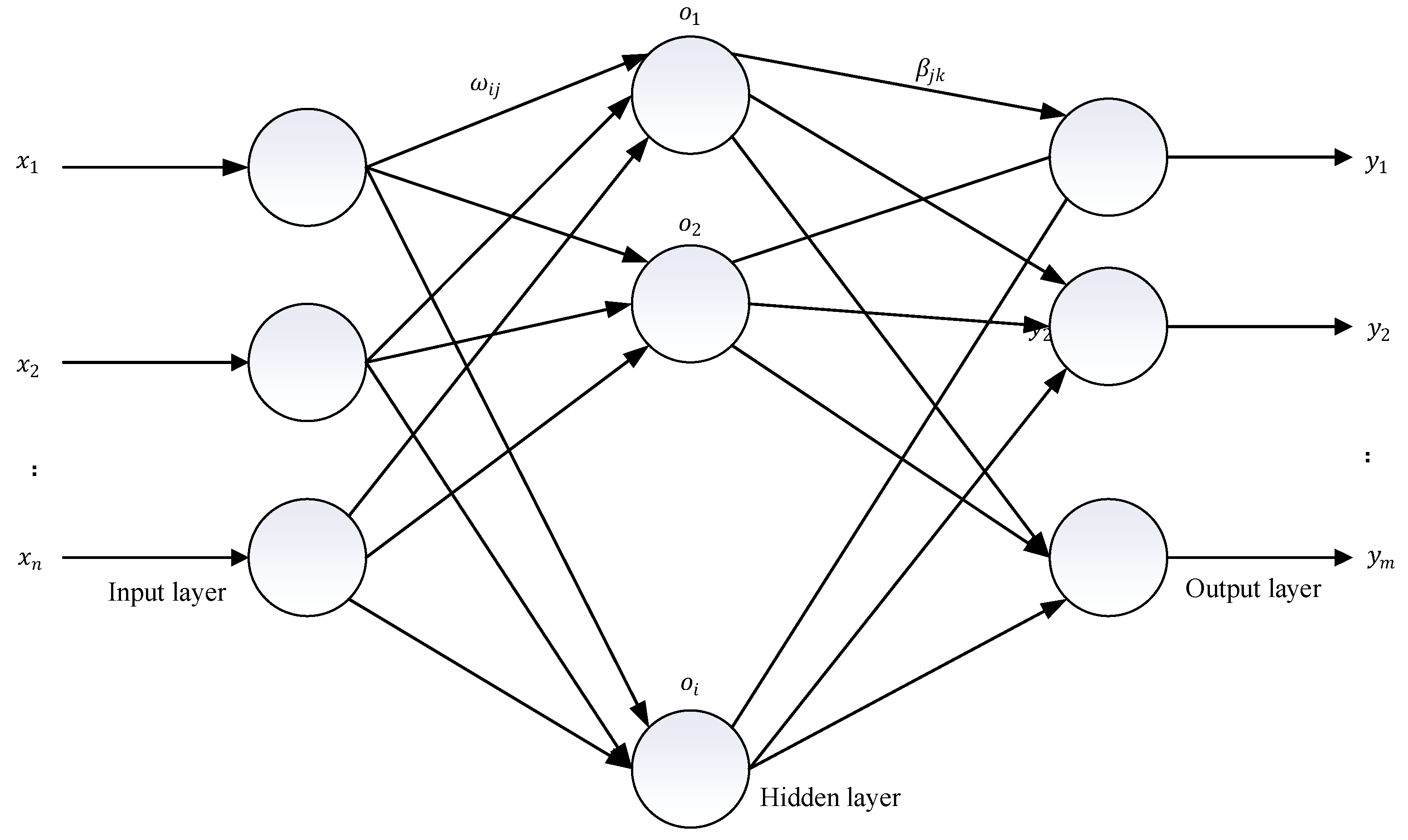
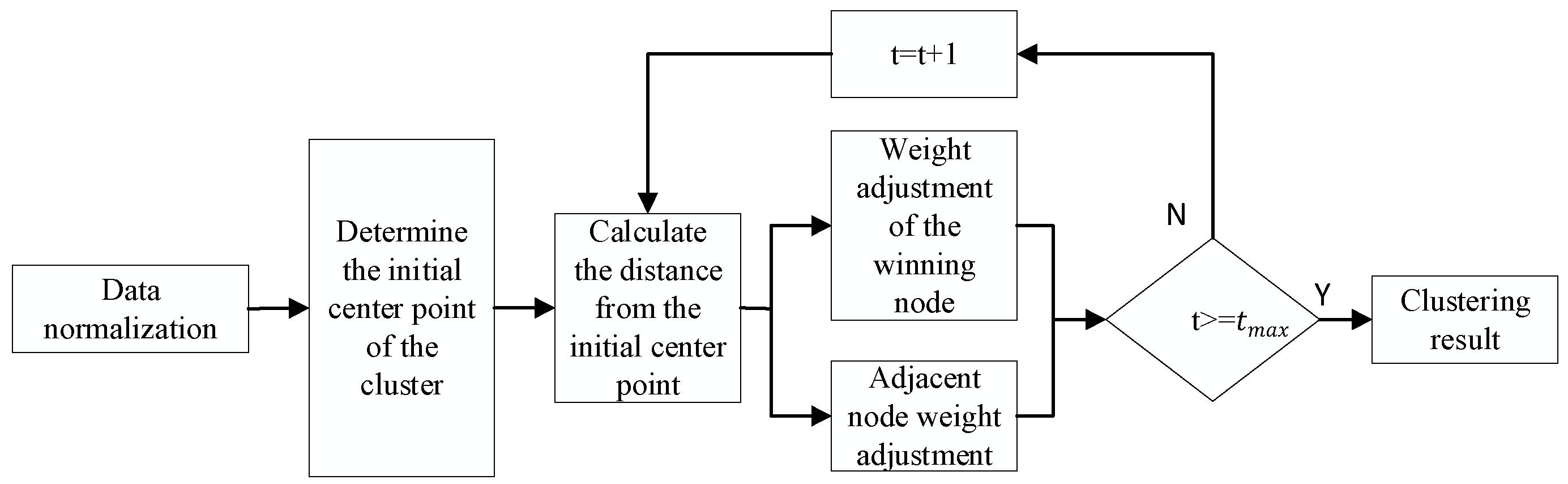
2.2. Kohonen Clustering Network

The Kohonen network was proposed by Finnish scientist Kohonen in 2001. It is a network called a self-organizing feature map, which belongs to the category of artificial neural network. It is an unsupervised learning algorithm in data mining and is widely used in cluster analysis problems. The clustering algorithm mainly involves how to measure the Euclidean distance between the input node, the winning output node, and what scheme to achieve clustering [25,26].

The Kohonen network topology has the following features.

• The network consists of two layers, namely an input layer and an output layer. The output layer is also called the competition layer and does not include the hidden layer.
• Each input node in the input layer is wholly connected to the output node.
• The output nodes are distributed in a two-dimensional structure, and there are lateral connections between the nodes.

The clustering process of the Kohonen network is as follows.

• Step 1: Data normalization.

For numerical variables, the difference in order of magnitude should be eliminated, all numerical variable values should be converted to the [0, 1] range. Finally,$p$ clustering variables$x\left(i=1,2,\dots ,p\right)$ with values ranging from 0 to 1 are obtained, and formula (1) is the data normalization formula [27].

$$X=\frac{x-x_{min}}{x_{max}-x_{min}}$$

(1)

• Step 2: Determine the initial center point of the cluster.

Similar to the K-Means algorithm [28], if the specified clustering item is $K$, the initial class center point of the $K$ class should be given randomly.

• Step 3: Calculate the distance [29].

Randomly input sample data $X\left(t\right)$, then calculate the Euclidean distance d between $X\left(t\right)$, and the K-type initial center store and find the closest center point, output node $W_c\left(t\right)$.

$$D\left(X\left(t\right),W_c\left(t\right)\right)=\sqrt{{\displaystyle \sum }_{i=1}^n{\left(X_i-W_i\right)}^2}$$

(2)

• Step 4: Adjust the position.

Adjusting the position involves two parts. The first part needs to change the algorithm, and the second part needs to determine the neighboring nodes of the “winning” node. The adjustment algorithm is similar to adjusting the network weights in the artificial neural network. The $p$ network weights between the $p$th input nodes and the $j$th output node at the time $t$ constitute [30]

$$W_j\left(t\right)=\left(W_{1j}\left(t\right),W_{2j}\left(t\right),\dots ,W_{pj}\left(t\right)\right)$$

(3)

The Kohonen network adjusts its weight based on the Euclidean distance between the sample and the class center, and adjusts the weight of the “winning” node $W_c\left(t\right)$ to

$$W_c\left(t+1\right)=W_c\left(t\right)+\eta t\parallel X\left(t\right)-W_c\left(t\right)\parallel$$

(4)

$\eta t$ is the learning rate at the time $t$. Since there are still lateral connections between the output nodes, the network weights of neighboring nodes around the “winning” node $W_c\left(t\right)$ need to be adjusted. Generally, a neighborhood radius needs to be specified, with $W_c\left(t\right)$ as the center of the circle. The output nodes within the specified radius will be regarded as neighboring nodes, and the weight adjustment formula for neighboring nodes $W_j\left(t\right)$ is

$$W_j\left(t+1\right)=W_j\left(t\right)+\eta t{h}_{jc}\left(t\right)\parallel X\left(t\right)-W_j\left(t\right)\parallel$$

(5)

In the formula, $h_{jc}\left(t\right)$ is the kernel function, which represents the distance measurement between the neighboring node and the “winning” node.

• Step 5: Determine whether the conditions for the end of the iteration are met.

If the conditions for the end of the iteration are not completed, return to the third step and repeat the three or four stages until the iteration conditions are met. The algorithm flow chart is shown in Figure 1.

2.3. Kernel Extreme Learning Machine (KELM)

The KELM is evolved from the ELM. The ELM only needs to set the number of gods in the hidden layer to obtain the optimal solution [31,32]. Compared with the traditional training method, this algorithm has a reasonable learning rate and good generalization performance. The ELM is a typical single-layer hidden layer feedforward neural network. The structure is shown in Figure 2. The input layer has $n$ neurons corresponding to the $n$ input vectors and the hidden layer has $l$ neurons. The output layer has $\mathrm{m}$ output variables. Among them, ${\omega }_{ij}$ represents the connection weight between the $i$th neuron in the input layer, and the $j$th neuron in the hidden layer. The specific learning process of the ELM has been described in detail in many papers [33,34,35,36,37].

Although the ELM can achieve good performance in most cases, the initial parameters of the hidden layer (including the number of connected nodes, the connection weight bias value, etc.) still have a significant influence on the classification accuracy of the ELM. The ELM learning objective function $F\left(x\right)$ can be expressed as a matrix

$$F\left(x\right)=h\left(x\right)\times \beta =H\times \beta =L,$$

(6)

where $x$ is the input vector, $h\left(x\right)$ is the output of the hidden layer node, $\beta$ is the output weight, and $L$ is the desired output.

The KELM can improve the prediction performance of the model based on preserving the advantages of the ELM [38,39,40]. There are $N$ pairs of classified training samples ($x_i,y_i$), where $i=1,2,\dots , N$. Training input data $x_i\in R^p$, $y_i\in R^m$ is the category label of $x_i$, where $m$ is the total number of categories. The output of $N$samples is called $Y={\left[y_1,y_2,\dots ,y_N,\right]}^T$ by the matrix. For the training sample $x_i$, it is assumed that there is a nonlinear mapping function $h \left(·\right)$, which can be mapped into a high-dimensional Hilbert space and becomes a characteristic mapping matrix $h \left(x_i\right)$. In the high-dimensional eigenspace, $N$ samples $h \left(x_i\right)$ are linearly separable. At this point, the KELM’s hidden layer neuron output can be expressed as [41]

$$H=\left[\begin{array}{c}h \left(x_1\right)\\ ⋮\\ h \left(x_N\right)\end{array}\right]$$

(7)

The output layer of the KELM has $m$ neurons, corresponding to $m$ classification categories, and the output layer is denoted by $y_i$. The weight matrix of the output layer is denoted as $\beta$, and the input data of $N$ training samples are received, respectively. There are $m$ neurons in the output layer, corresponding to $m$ classification categories, respectively. The KELM training can represent an optimization problem [42]

$$\underset{\beta }{\min }\frac{1}{2}\parallel {\beta }^2\parallel +\frac{C}{2}\parallel {\epsilon }_i\parallel {}^2$$

$$s_{.}{t}_{.} h \left(x_i\right)\beta =y_i^T-{\epsilon }_i^T, i=1,2,\dots , N$$

(8)

where $C$ is the penalty coefficient and ${\epsilon }_i$ is the classification error. The Lagrange function of optimization problem is denoted as [43]

$$L=\frac{1}{2}\parallel {\beta }^2\parallel +\frac{c}{2}\parallel {\epsilon }_i\parallel {}^2-{\displaystyle \sum }_{i=1}^N{\displaystyle \sum }_{j=1}^m{\alpha }_{i,j}\left(h\left(x_i\right){\beta }_j-y_{i,j}+{\epsilon }_{i,j}\right)$$

(9)

where the Lagrange multiplier ${\alpha }_i\in R^m$. According to the Kuhn–Tucker optimality theory, take the first-order partial derivatives of Equation (9) for variables ${\beta }_i$, ${\epsilon }_i$, ${\alpha }_i$, respectively, and let them be zero. The output layer weight of KELM can be solved as:

$$\beta =H^T{\left(H{H}^T+\frac{1}{C}\right)}^{-1}Y.$$

(10)

For $s$ test sample sets $x^{\ast }={\left[x_1^{\ast },x_2^{\ast },\dots ,x_s^{\ast }\right]}^T$, where $x_i^{\ast }\in R^P$, the classification output of KELM is

$$y^{\ast }=h\left(x^{\ast }\right)\beta =h\left(x^{\ast }\right)H^T{\left(H{H}^T+\frac{1}{C}\right)}^{-1}Y.$$

(11)

where $I$ is the identity matrix of order $N$. For two vectors $h\left(x_i\right)$ and $h\left(x_j\right)$ in Hilbert space, their inner product can be calculated by the kernel function $K\left(■\right)$, denoted as

$$h\left(x_i\right)h{\left(x_j\right)}^T=K\left(x_i,x_j\right).$$

(12)

According to Equation (12)

$$H{H}^T=K=K\left(X,X\right)=\left[\begin{array}{c}K\left(x_1,x_1\right) K\left(x_1,x_2\right)\cdots K\left(x_1,x_N\right)\\ K\left(x_2,x_1\right) K\left(x_2,x_2\right)\cdots K\left(x_2,x_N\right)\\ ⋮ ⋮ ⋮\\ K\left(x_N,x_1\right) K\left(x_N,x_2\right) \cdots K\left(x_N,x_N\right)\end{array}\right].$$

(13)

In the same way with

$$h\left(x^{\ast }\right)H^T=K^{\ast }=K\left(x^{\ast },X\right).$$

(14)

Substituting Equations (12) and (13) into Equation (11), the classification output of the KELM is

$$y^{\ast }=K^{\ast }{\left(K+\frac{1}{C}\right)}^{-1}Y.$$

(15)

$K$ is the kernel function. Radial basis kernel function, linear kernel function, polynomial kernel function, and wavelet kernel function are commonly used parts of the KELM, as shown in

Table 1. The prediction results of different prediction models, $x$ and $z$ are both input vectors.

Type	Expressions	Parameters
Radial Basis Kernel	$K\left(x,z\right)=e^{-\gamma \parallel x-z{\parallel }^2}$	$\gamma =\frac{1}{2{\sigma }^2}$ $\sigma$: Free parameters.
Linear Kernel	$K\left(x,z\right)=x^{T}z+c$	$c$: Constant
Polynomial Kernel	$K\left(x,z\right)={\left(\alpha x^{T}z+c\right)}^d$	$\alpha$: Slope $c$: Constant $d$: Number of polynomials
Wavelet Kernel	$K\left(x,z\right)={\displaystyle {\displaystyle \prod }_{i=1}^N}h\left(\frac{\left(x_i-c\right)}{a}\right)h\left(\frac{z_i-c}{a}\right)$	$a$: Wavelet expansion factor $c$: Translation factor $h\left(x\right)=\cos \left(1.75x\right)\exp \left(-\frac{x^2}{2}\right)$

.

The linear kernel function is generally expressed as

$$K\left(x,z\right)=x^{T}z+c$$

(16)

It is the inner product of two vectors, one transpose, so the linear kernel does not do anything to the data which means it does not map the data to higher dimensions, but in many cases the simplest is the best. The linear kernel function is very simple to operate and convenient to calculate, especially in the case of large sample data, the linear kernel function can play a good effect.

The polynomial kernel function is generally expressed as

$$K\left(x,z\right)={\left(\alpha x^{T}z+c\right)}^d.$$

(17)

Polynomial kernel function is increased on the basis of linear kernel function parameters such as α and d. These parameters can be specified by the user, and the polynomial kernel function also has very good understanding. According to Formula 1, $\alpha$ is for the internal product for scaling, and $c$ is a constant term, to add and subtract in the adjustment, $d$ is to control the number of times. The transformation is an additional transformation of the inner product of $x$ and $z$. Since the polynomial kernel function is an additional transformation based on the inner product of $x$ and $z$, it is less functional.

The radial basis kernel function is generally expressed as

$$K\left(x,z\right)=e^{-\gamma \parallel x-z{\parallel }^2}.$$

(18)

When the radial basis kernel function is expanded, the denominator $2{\sigma }^2$ can be obtained

$$K\left(x,z\right)=e^{\left|-x^2\right|}{e}^{\left|-z^2\right|}{e}^{\left|2xz\right|}.$$

(19)

When Taylor expansion is performed using Formula (19), it can obtain

$${\displaystyle \sum }_{n=0}^{\infty }{e}^{\left|-x^2\right|}\sqrt{\frac{2n}{n!}}{\left(x\right)}^n{\displaystyle \sum }_{n=0}^{\infty }{e}^{\left|-z^2\right|}\sqrt{\frac{2n}{n!}}{\left(z\right)}^n=K\left(x,z\right)=\phi \left(x\right)\phi \left(z\right)$$

(20)

A seemingly simple formula such as radial basis kernel function can be extended to an infinite number of dimensions for both $x$ and $z$ passed in. The higher the latitude, the more complex the model, and the stronger the function (if the fitting is not considered).

The smaller $\sigma$ is, the larger the radial basis kernel value will be for each pair of sample points. The farther the distance between the samples is, the more inclined the model will be to place these different sample points into different classes. If $\sigma$ is large, the sample points are calculated to be close to each other, and the model tends to place them in the same category.

Wavelet kernel function has great advantages in signal processing, image processing, and sound processing.

Through the transformation analysis of four kinds of kernels, radial basis kernels can be a suitable choice for the KELM theoretically. This study will verify this conclusion in Section 4.2.

3. Optimized Kernel Extreme Learning Machine

The KELM needs to optimize the regularization coefficient $C$ and the kernel parameter $S$; these two parameters have a significant influence on the prediction results [44]. Meta-heuristic algorithm is a method for solving the optimal solution of complex optimization problems, which is based on the mechanism of computational intelligence [45]. Meta-heuristic algorithms include simulated annealing algorithm [46], tabu search algorithm [47], genetic algorithm [48], evolution strategy, differential evolution algorithm, ant colony algorithm, gray wolf algorithm, particle swarm algorithm, and so on. Annealing is a metal heat treatment process, which means that the metal is slowly heated to a certain temperature and maintained for a sufficient time, and then cooled at an appropriate speed. The purpose is to reduce the hardness and stabilize the dimensions. For example, the simple genetic algorithm has disadvantages such as poor local search ability and premature convergence. To overcome these shortcomings, the simulated annealing algorithm with good local search ability is combined with a genetic algorithm. Wang et al. [49] proposed a new genetic simulated annealing algorithm to optimize the parallel disassembly balance model, improving disassembly efficiency and profit. The results show that the simulated annealing genetic algorithm has more advantages, and good practical application ability. Dereli [37] used the gray wolf optimization algorithm to solve the most basic inverse kinematics problem in robotics. The gray wolf optimization algorithm produces similar results to other group-based algorithms, but the improved gray wolf algorithm has better values and makes the result more convergent. Tabu search is a modern heuristic algorithm, a search method used to escape the optimal local solution. Tabu search first creates an initial solution and then continuously adjusts and moves to improve the quality of the solution. It can prevent repeated searches for the same target to find the optimal solution process [50]. Different optimization algorithms have different optimization effects on the same model, so this study needs to find a more appropriate optimization algorithm [51].

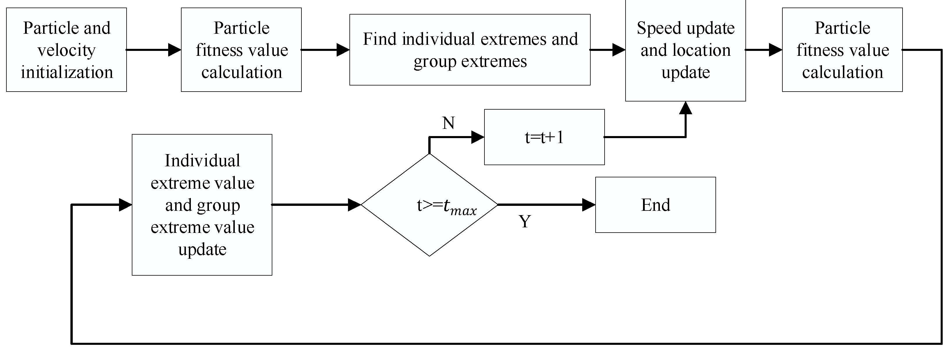
3.1. Particle Swarm Optimization to Optimize the KELM

The PSO is an evolutionary computation technology derived from the study of predation behavior of birds. The basic idea of the PSO algorithm is to find the optimal solution through collaboration and information sharing between individuals in the group [52]. The advantage of the PSO is that it is simple and easy to implement and does not have many parameter adjustments. At present, it has been widely used in face images in computer vision [53], neural network training [54], and in breast cancer prediction [55]. The PSO algorithm simulates the birds in a flock of birds by designing a massless particle. The particle only has two attributes: speed and position. Speed represents the speed of movement, and position defines the direction of motion. Each particle searches for the optimal solution individually in the search space, and records it as the current individual extreme value, The extreme values are shared with the whole particle swarm, and the individual extreme values are regarded as the group extreme values. In each iteration, the particle updates its speed and position through individual extreme values and extreme global values. The update formula is as follows

$$V_{id}^{k+1}=\omega V_{id}^k+c_1{r}_1\left(P_{id}^k-X_{id}^k\right)+c_2{r}_2\left(P_{gd}^k-X_{id}^k\right)$$

(21)

$$X_{id}^{k+1}=X_{id}^k+V_{id}^{k+1}$$

(22)

In the formula, $\omega$ is the inertial weight; $d=1,2,\cdots ,D$; $i=1,2,\cdots ,n$; $k$ is the current iteration number; $V_{id}$ is the velocity of the particle; $c_1$ and $c_2$ are non-negative constants called acceleration factors; and $r_1$ and $r_2$ are random numbers distributed between 0 and 1. To prevent the blind search of particles, it is generally recommended to limit the velocity of its position to a certain interval. Figure 3 is a flow chart of the PSO.

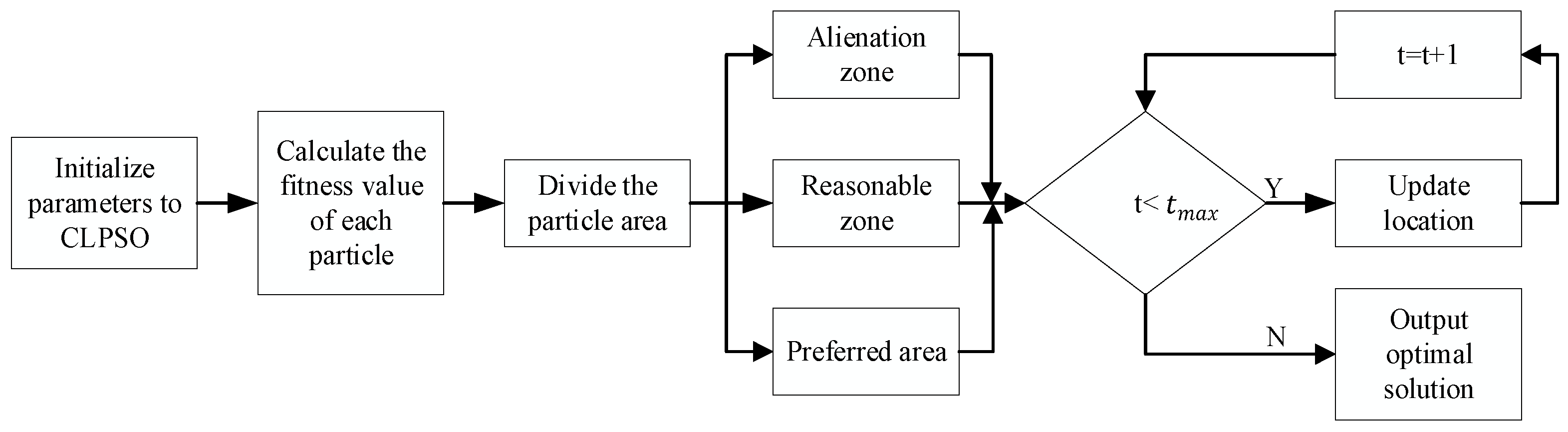
3.2. Particle Swarm Optimization Algorithm Based on Competitive Learning (CLPSP) to Optimize the KELM

Traditionally, the PSO also has some shortcomings. As the difficulty of the optimization problem increases, the efficiency of the PSO in finding excellent particles will become lower and lower. At the same time, the PSO algorithm also has premature convergence, and it is easy to fall into a local optimum [56]. Therefore, the CLPSO was proposed in recent years, The main idea is to divide the dynamics of the particle swarm into three parts, namely the alienation zone, the rational zone, and the optimal zone. The particles in each area correspond to a particle update formula, so that each particle can adjust its state in time and move towards the optimal global state. The optimal area is relatively close to the best position of the population. To prevent falling into the local optimum, the Cauchy formula needs to be used for self-mutation. The particle update formula of the optimal area is

$$x_{ij}^p\left(t+1\right)=x_{ij}^p\left(t\right)·\left(1+n_t·C\left(0,1\right)\right)$$

(23)

$$n_t=\frac{t_{max}-t}{t_{max}}$$

(24)

$n_t$ is the parameter that controls the asynchronous variable length, $C\left(0,1\right)$ is the random number generated by the Cauchy distribution function, $x_{ij}^p\left(t\right)$ represents the particle’s position in the preferred area, $t_{max}$ is the maximum number of iterations, and $t$ is the current number of iterations. The particles in the alienation zone are far away from the optimal position of the population and it is necessary to accelerate the movement speed of the particles to the optimal solution. The particle position update formula in the alienation zone is

$$x_{ij}^A\left(t+1\right)=c_1{x}_{ij}^A\left(t\right)+c_2(x_{ij}^A\left(t\right)-x_{kj}^P\left(t\right))+c_3\alpha \left(\overline{f}-x_{ij}^A\left(t\right)\right)$$

(25)

In the formula, $c_1$, $c_2$, and $c_3$ are acceleration weights, $\alpha$ is a small greater than 0 number, and the particle position update in the alienation zone is also affected by the center position. The particle in the reasonable area needs to weigh the global search and local development. Therefore, there are two particle position update formulas for particles in the reasonable site, when the particle does not fall into the local optimum, Formulas (21) and (22) are used to update the position of the particle swarm. When the particles in the alienation zone fall into the local optimum, it is the current fitness value of the particle and the previous generation particle fitness. When the values are the same, use Formulas (23) and (24) to update the position. The algorithm flow is shown in Figure 4.

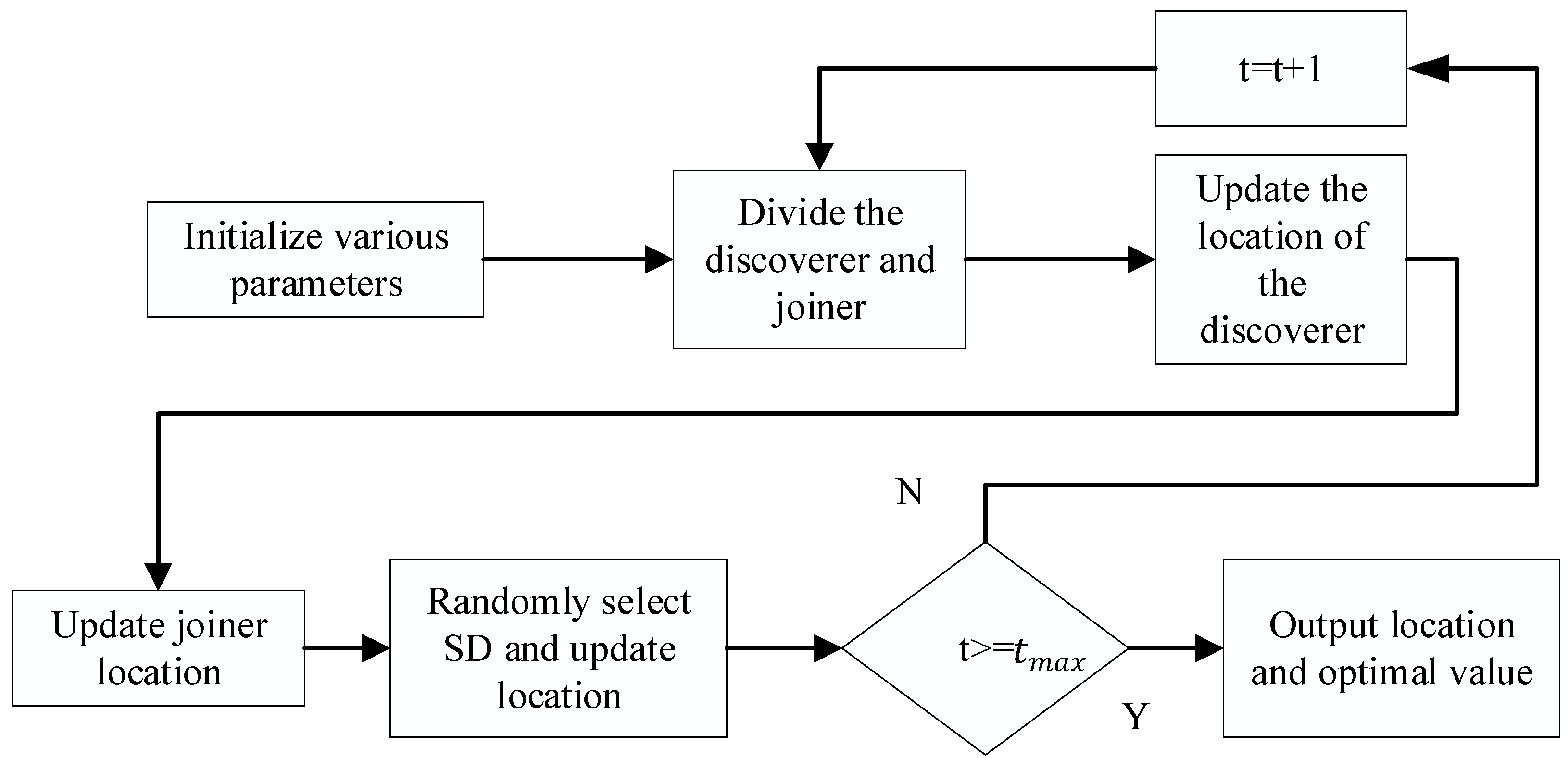
3.3. Sparrow Search Algorithm (SSA) to Optimize the KELM

The SSA is inspired by natural biological sparrows’ food-seeking behavior and anti-reconnaissance behavior. It has high global search capabilities and local development capabilities [57]. The SSA is used to optimize the capacity configuration of wind energy–solar diesel accumulators [58], the path planning of mobile robots [59], and optimize the back propagation (BP) algorithm [60]. There are three identities of sparrows in the sparrow population. The discoverer is responsible for providing foraging locations for the entire population, the joiner uses the discoverer to find food and the more alert is accountable for protecting the population’s safety. Six rules are observed throughout the population:

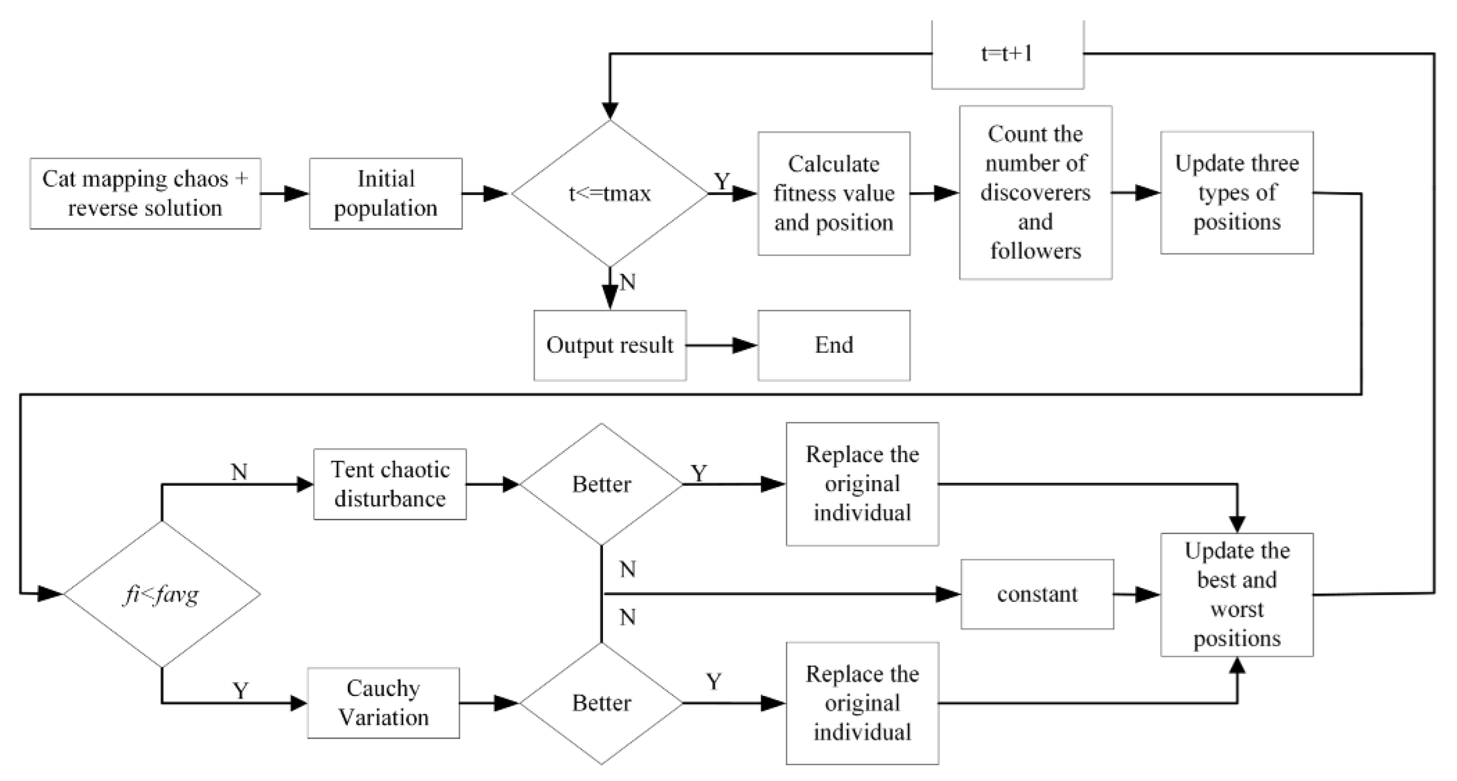
• Under normal circumstances, the discoverer has a relatively high energy reserve, and the energy reserve corresponds to adaptability.
• The identity between the discoverer and the joiner changes dynamically, and their ratio remains unchanged.
• The position of the joiner is proportional to the energy, the lower the power, the more likely it is to fly to other places for food.
• Joiners will always find discoverers who provide good food and fight with them.
• After the alarm value is greater than the safe value, the discoverer will lead the sparrow population into the safe area.
• When the entire population moves, the sparrows at the edge of the people will quickly move to a safe place. In contrast, the sparrows inside the population will randomly move to the surrounding sparrows. The location update of the discoverer

$$X_{i,j}^{t+1}=\left\{\begin{array}{c}{X}_{i,j }^{t+1}·exp\left(-\frac{i}{\alpha ·t_{max}}\right)if R_2<ST\\ X_{i,j }^{t+1}+Q·L if R_2\ge ST\end{array}\right.$$

(26)

where $t$ represents the current number of iterations, $t_{max}$ represents the maximum number of iterations, $X_{i,j}$ represents the location information of the sparrow, $\alpha$ is a random number between 0 and 1, $R_2$ is an early warning value of 0 to 1,$ST$ is a safe value of 0.5 to 1, and $Q$ follows the normal distribution. The follower location update formula

$$X_{i,j}^{t+1}=\left\{\begin{array}{c}Q·exp\left(\frac{X_{worst}-X_{i,j}^t}{i^2}\right) if i>\raisebox{1ex}{$n$}\!\left/ \!\raisebox{-1ex}{$2$}\right.\\ X_p^{t+1}+\left|X_{i,j}^t-X_p^{t+1}\right|·A^{+}·L otherwise\end{array}\right.$$

(27)

Among them, Xp is the best location occupied by all discoverers, and $X_{worst}$ represents the worst position globally. The algorithm flow chart is shown in Figure 5.

3.4. Adaptive Mutation Sparrow Search Algorithm (AMSSA) to Optimize the KELM

The SSA has problems in that it is easy to fall into local extreme points in the early stage and the accuracy of finding the optimal value in the later stage is not high [61,62]. Therefore, the AMSSA is proposed. First, to improve the randomness and richness of the whole population, the cat mapping chaotic sequence is used to initialize the entire population, and the cat mapping expression is

$$\left[\begin{array}{c}{y}_{i+1}\\ w_{i+1}\end{array}\right]=\left[\begin{array}{cc}1& {\alpha }_1\\ b_1& {\alpha }_1{b}_1+1\end{array}\right]\left[\begin{array}{c}{y}_i\\ w_i\end{array}\right]mod1$$

(28)

where ${\alpha }_1$ and $b_1$ are arbitrary real numbers and $mod1$ means finding the decimal part of ${\alpha }_1$. Perform tent chaotic perturbation or Cauchy mutation according to the fitness value of the population individuals, this is to prevent individuals from being too scattered or too concentrated. The expression of the tent chaotic map is

$$z_{i+1}=\left\{\begin{array}{c}2z_i+rand\left(0,1\right)\times pop, 0\le z\le 0.5\\ 2\left(1-z_i\right)+rand\left(0,1\right)\times pop,0.5\le z\le 1\end{array}\right.$$

(29)

The random variable $rand\left(0,1\right)\times pop$ is improved on the original basis [63], and $pop$ is the number of particle populations. The Cauchy variation formula is

$$mutationx=x\left(1+tan\left(\pi \left(u-0.5\right)\right)\right)$$

(30)

where $x$ is the original particle position and $u$ is a random number in the interval [0, 1] range. The algorithm flow chart is shown in Figure 6.

4. Result

The 17 blood indicators included: white blood cell count, lymphocyte count, monocyte count, neutrophil count, eosinophil count, basophil count, red blood cell count, hemoglobin concentration, platelet count, total protein, albumin globulin, prothrombin time (PT), international normalized ratio (INR), activated partial thromboplastin time (APTT), thrombin time (TT), and fibrinogen (FIB). Blood data were collected from all patients before treatment, 108 were still alive at the end of the follow-up and 232 were dead at the end of the follow-up. The end points were the time of death after treatment and the end of follow-up. Level 1 is positive and level 2 is negative. The number of positive patients was 180 and the number of negative patients was 160.

Datasets are not easy to obtain. If you want to access them, please email [email protected].

In order to evaluate the performance of the proposed model, 10-fold cross-validation was applied to all schemes. The initial sample was divided into 10 subsamples, 1 single subsample was reserved as the data of the validation model, and the other 9 samples were used for training. Cross-validation is repeated 10 times, once for each subsample, averaging the results of 10 times or using other combinations, resulting in a single estimate. The advantage of this method lies in the repeated use of randomly generated subsamples for training and verification, and the results are verified once each time. Evaluation indicators include:

Accuracy ($ACC$): The probability that all samples are correctly predicted.

$$ACC=\left(TP+TN\right)/\left(TP+TN+FN+FP\right).$$

(31)

$TP$ is the number of positive examples correctly classified; $TN$ is correctly divided into the number of negative cases; $FP$ was incorrectly classified as the number of positive examples; and $FN$ is correctly divided into the number of negative cases.

Sensitivity ($SEN$): The recognition ability of the classifier to positive cases is measured.

$$SEN=TP/\left(TP+FN\right).$$

(32)

Specificity ($SPE$): The recognition ability of the classifier to negative cases is measured.

$$SPE=TN/\left(FP+TN\right).$$

(33)

$FPR$: False-positive rate:

$$FPR=FP/\left(FP+TN\right).$$

(34)

$FNR$: False-negative rate:

$$FNR=FN/\left(FN+TP\right)$$

(35)

4.1. Data Clustering

The research will input specific data into the Kohonen network. In this network training, the learning rate is 0.05 to 0.2, the neighborhood radius is 1.5 to 0.8, and the number of iterations is 10,000.

Table 2. Clustering result, the first row represents categories, and the second row represents the number of similar categories.

Classification category	1	2	3	4	5
Number of samples	82	76	53	50	79

shows the number of samples for each type of the Kohonen network and performs Cox regression to verify the relevance of the classification results, the p-value of the 17 blood index combinations in each group is much less than 0.001, indicating that the combination of blood indicators has a significant relationship with the patient’s survival time.

4.2. Choice of Kernel Function of the KELM

Choosing the kernel function type of the KELM is an essential part of analyzing the survival risk level of esophageal cancer. In the Windows 10 operating environment, MATLAB2018b software simulation software was used, and the prediction results obtained from 17 blood indicators of 340 patients were used to select the kernel function.

The specific results are shown in

Table 3. Prediction result of different kernel functions. SEN: Number of correct and positive validation predictions, as a percentage of positive numbers. SPE: The number of predictions that are negative and correct, as a percentage of the actual total number of negative purposes. FPR: False-positive rate. FNR: False-negative rate.

Kernel Function Type	Risk Level	$\mathit{A}\mathit{C}\mathit{C}$ (%)	$\mathit{A}\mathit{C}\mathit{C}$ (%)	$\mathit{S}\mathit{E}\mathit{N} (\%)$	$\mathit{S}\mathit{P}\mathit{E} (\%)$	$\mathit{F}\mathit{P}\mathit{R} (\%)$	$\mathit{F}\mathit{N}\mathit{R} (\%)$
Radial basis function	Level 1	70.0	68.5	70.0	66.7	33.3	30.0
	Level 2	66.7
Linear	level 1	60.0	53.4	60.0	45.5	54.5	40.0
	level 2	45.5
Polynomial	level 1	65.0	54.8	65.0	42.4	57.6	35.0
	level 2	42.4
Wavelet	level 1	37.5	43.8	37.5	51.5	48.5	62.5
	level 2	51.5

. By comparing the four kernel functions, RBF kernel function showed better prediction accuracy than the other three kernel functions in terms of accuracy, sensitivity, specificity, false positive, and false negative. RBF-ELM has an accuracy of 68.5%, sensitivity of 70.0%, specificity of 66.7%, false positive of 33.3%, and false negative of 30.0%. Therefore, RBF is adopted as the kernel function of KELM.

4.3. Optimization Algorithm Optimization Results

The PSO has the advantages of fast convergence, especially in the early stage of the algorithm, but it also has the disadvantages of low accuracy and easy divergence. If the acceleration coefficient, maximum velocity, and other parameters are too large, the particle swarm may miss the optimal solution, resulting in non-convergence of the algorithm. In the case of convergence, because all particles move to the direction of the optimal solution, the particles tend to be identical, which makes the late convergence speed slow down. After convergence reaches a certain precision, the optimization cannot be continued. In order to achieve the best balance between global exploration and local development, the CLPSO was proposed. In the CLPSO, by dynamically dividing the population into three subgroups and designing different evolution mechanisms for the particles in each subgroup, we increase strong population diversity, improve the local search ability, and avoid the particle for the global optimal particle blindly following, which overcomes the defect that it is easy to fall into the local optimum when solving a multi-peak problem. The structure of the CLPSO is complex and the operation time of the program is long. The SSA is mainly inspired by the foraging behavior and anti-predation behavior of sparrows. The algorithm is novel and has the advantages of strong searching ability, fast convergence speed, and relatively simple structure. Although easy to achieve, how to adjust the control parameters between the parts and how to ensure that the three parts can better cooperate with each other is a problem that must be considered. Based on the SSA, the AMSSA is proposed by introducing chaotic mapping, Cauchy variation and adaptive adjustment strategy of the number of explorers’ followers. Firstly, cat mapping chaos speeds up the convergence of population initialization. Secondly, the adaptive explorer–follower adjustment strategy makes the algorithm focus on global optimization in the early stage and local optimization in the later stage, which improves the convergence accuracy. Finally, tent mixed disturbance and Cauchy variation make the algorithm jump out of the local extreme point, which makes the AMSSA algorithm have higher searching accuracy, and stronger searching ability compared with the SSA algorithm.

Four optimization algorithms have been compared in this article (the PSO, the CLPSO, the SSA, and the AMSSA),

Table 4. Optimization results of different optimization models. SEN: Number of correct and positive validation predictions, as a percentage of positive numbers. SPE: The number of predictions that are negative and correct, as a percentage of the actual total number of negative purposes. FPR: False-positive rate. FNR: False-negative rate.

Predictive Model	Risk Level	$\mathit{A}\mathit{C}\mathit{C}$ (%)	$\mathit{A}\mathit{C}\mathit{C}$ (%)	$\mathit{S}\mathit{E}\mathit{N} (\%)$	$\mathit{S}\mathit{P}\mathit{E} (\%)$	$\mathit{F}\mathit{P}\mathit{R} (\%)$	$\mathit{F}\mathit{N}\mathit{R} (\%)$	Running Time(s)
KELM	level 1	70.0	68.5	70	66.7	33.3	30.0	3.20
	level 2	66.7
SSA-KELM	level 1	90.0	89.0	90	87.8	12.1	10.0	15.38
	level 2	87.8
PSO-KELM	level 1	92.5	84.9	93	75.6	24.2	7.5	17.56
	level 2	75.6
CLPSO-KELM	level 1	95.0	89.0	95	81.8	18.2	5	14.12
	level 2	81.8
AMSSA-KELM	level 1	95.0	91.8	95	87.8	12.1	5	10.26
	level 2	87.8

shows that the four optimization algorithms optimize the KELM to have better results than the KELM alone. From the perspective of overall accuracy, the SSA-KELM and the CLPSO-KELM achieve 89% accuracy, while the AMSSA-KELM breakthrough 90% and reach 91.8%. In terms of specificity, the SSA-KELM and the AMSSA-KELM are the highest among the four algorithms, reaching 87.8, while in terms of sensitivity, the AMSSA-KELM and the CLPSO-KELM are 95%. In terms of false positive, both the SSA-KELM and the AMSSA-KELM reached the lowest value of 12.1%, indicating that the misdiagnosis rate of these two models was the lowest. In terms of false negative, the CLPSO-KELM and the AMSSA-KELM only had 5%, indicating that the missed diagnosis rate of the two models was the lowest. By comparing these aspects, the AMSSA-KELM shows better classification performance, thus proving the effectiveness of the AMSSA-KELM model.

4.4. Results Predicted by Different Models

The paper [64] mentioned the ABC-SVM prediction model. First, the method extracted nine blood indicators (white blood cell count (WBC), lymphocyte (LYMPH), monocytes (MONO), neutrophil count (NEUT), eosinophils (EO), basophilic (BASO), red blood cell count (RBC), PT, and INR). Finally, the optimization algorithm was used to improve the SVM to improve the prediction accuracy of the model rate. Another paper [65] proposed to use the TLRF prediction model to assess the accuracy of youth violence or crime. This method mainly uses three sets of predictors to predict three outcomes: arrest, conviction, and imprisonment. Model 1 is based on social demographic statistics, model 2 adds behaviors or scenarios, and model 3 adds emotional and environmental risk factors, which significantly improves the prediction of someone’s arrest, conviction, and imprisonment. In this paper, data are brought into the two models the GP-SVM and the Cox-LMM in the introduction, and the models in the above two literatures, the results are shown in Table 4.

As shown in

Table 5. The prediction results of different prediction models. $SEN$: Number of correct and positive validation predictions, as a percentage of positive numbers. $SPE$: The number of predictions that are negative and correct, as a percentage of the actual total number of negative purposes. $FPR$: False-positive rate. $FNR$: False-negative rate.

Predictive Model	Risk Level	$\mathit{A}\mathit{C}\mathit{C}$ (%)	$\mathit{A}\mathit{C}\mathit{C}$ (%)	$\mathit{S}\mathit{E}\mathit{N} (\%)$	$\mathit{S}\mathit{P}\mathit{E} (\%)$	$\mathit{F}\mathit{P}\mathit{R} (\%)$	$\mathit{F}\mathit{N}\mathit{R} (\%)$	Running Time(s)
AMSSA-KELM	level 1	95.0	91.8	95.0	87.8	12.1	5.0	10.26
	level 2	87.8
ABC-SVM	level 1	87.5	81.8	87.5	72.7	27.3	12.5	10.38
	level 2	72.7
TLRF	level 1	57.5	61.6	57.5	66.7	33.3	42.5	20.15
	level 2	66.7
GP-SVM	level 1	90.0	83.6	90.0	75.6	24.2	10.0	30.50
	level 2	75.6
Cox-LMM	level 1	62.5	61.6	62.5	60.6	39.4	37.5	15.41
	level 2	60.6

, in this study, the AMSSA-KELM showed better performance in accuracy, sensitivity, specificity, false positive, false negative, and operation time, delivering a better classification performance.

5. Discussion

In this study, the KELM with RBF as the kernel function was selected, and the AMSSA was used to optimize the KELM to achieve better results. Compared with other three optimization algorithms, the AMSSA-KELM prediction model proposed in this paper has certain competitiveness. This indicates that the AMSSA-KELM model can help doctors customize personalized treatment plans for patients to a certain extent. Due to the cross and overlap of the distribution of esophageal cancer patient data, each model only processes independent samples, which makes the processing accuracy of boundary patient input low, and this problem deserves further study.

6. Conclusions

To be able to more accurately distinguish the survival risk level of esophageal cancer, a combination method of the Kohonen clustering network and KELM is proposed in this article. This method uses the Kohonen clustering network to cluster 340 samples, divides two risk levels with a five-year survival period, and in view of the influence of different activation functions on KELM modeling, in this study, by extending the transformation of four activation functions (radial basis kernel, linear kernel, polynomial kernel, and wavelet kernel), it is proved that the RBF kernel function is more theoretically and experimentally suitable for this study. The PSO-KELM, the CLPSO-KELM, the SSA-KELM, and the AMSSA-KELM improve the prediction accuracy rate of esophageal cancer. By comparing accuracy, specificity, sensitivity, false positive, false negative, and operation time of the four algorithms, the results show that the AMSSA-KELM survival risk prediction model in this study has a better performance than the other three prediction models. Due to the complexity of esophageal cancer patient data, some samples are not completely classified into the specified intervals and there is some ambiguity, thus leading to a lower prediction accuracy for patients at the boundary position, and this issue deserves in-depth study in the future.

References

1. Anzolin, A.; Isenburg, K.; Toppi, A.; Yucel, M.; Ellingsen, D.; Gerber, J.; Ciaramidaro, A.; Astolfi, L.; Kaptchuk, T.; Napadow, V. Patient-Clinician Brain Response During Clinical Encounter and Pain Treatment. In Proceedings of the 2020 42nd Annual International Conference of the IEEE Engineering in Medicine & Biology Society (EMBC), Montreal, QC, Canada, 20–24 July 2020; p. 19964246. [Google Scholar]
2. Qiu, H.; Cao, S.; Xu, R. Cancer incidence, mortality, and burden in China: A time-trend analysis and comparison with the United States and United Kingdom based on the global epidemiological data released in 2020. Cancer Commun. 2021, 41, 1037–1048. [Google Scholar] [CrossRef] [PubMed]
3. Anji, R.; Soni, B.; Sudheer, R. Breast cancer detection by leveraging Machine Learning. ICT Express 2020, 6, 320–324. [Google Scholar]
4. Chen, D.; Fan, N.; Jun, X.; Wang, W.; Qi, R.; Jia, Y. Multiple primary malignancies for squamous cell carcinoma and adenocarcinoma of the esophagus. J. Thorac. Dis. 2019, 11, 3292–3301. [Google Scholar] [CrossRef] [PubMed]
5. Alberti, M.; Ruiz, J.; Fernandez, M.; Fassola, L.; Caro, F.; Roldan, I.; Paulin, F. Comparative survival analysis between idiopathic pulmonary fibrosis and chronic hypersensitivity pneumonitis. Pulmonology 2020, 26, 3–9. [Google Scholar] [CrossRef]
6. Yu, X.; Wang, T.; Huang, S. How can gene-expression information improve prognostic prediction in TCGA cancers: An empirical comparison study on regularization and mixed Cox models. Front. Genet. 2020, 11, 920. [Google Scholar] [CrossRef]
7. Emura, T.; Hsu, W.; Chou, W. A survival tree based on stabilized score tests for high-dimensional covariates. J. Appl. Stat. 2021, 1–27. [Google Scholar] [CrossRef]
8. Gaudart, J.; Giusiano, B.; Huiart, L. Comparison of the performance of multi-layer perceptron and linear regression for epidemiological data. Comput. Stat. Data Anal. 2004, 44, 547–570. [Google Scholar] [CrossRef] [Green Version]
9. Wang, B.; Ding, X.; Wang, F. Determination of polynomial degree in the regression of drug combinations. IEEE/CAA J. Autom. Sin. 2017, 4, 41–47. [Google Scholar] [CrossRef]
10. Witten, D.; Tibshirani, R. Survival analysis with high-dimensional covariates. Stat. Methods Med. Res. 2010, 19, 29–51. [Google Scholar] [CrossRef]
11. Van Wieringen, W.; Kun, D.; Hampel, R.; Boulesteix, A. Survival prediction using gene expression data: A review and comparison. Comput. Stat. Data Anal. 2009, 53, 1590–1603. [Google Scholar] [CrossRef]
12. Emura, T.; Matsui, S.; Chen, H. compound.Cox: Univariate feature selection and compound covariate for predicting survival. Comput. Methods Programs Biomed. 2019, 168, 21–37. [Google Scholar] [CrossRef] [PubMed]
13. Hussein, M.; Everson, M.; Haidry, R. Esophageal squamous dysplasia and cancer: Is artificial intelligence our best weapon? Baillière’s Best Pract. Res. Clin. Gastroenterol. 2020, 52, 101723. [Google Scholar] [CrossRef] [PubMed]
14. Ting, W.; Chang, H.; Chang, C.; Lu, C. Developing a novel machine learning-based classification scheme for predicting SPCs in colorectal cancer survivors. Appl. Sci. 2020, 10, 1355. [Google Scholar] [CrossRef] [Green Version]
15. Chang, S.R.; Liu, Y.A. Breast cancer diagnosis and prediction model based on improved PSO-SVM based on gray relational analysis. In Proceedings of the International Symposium on Distributed Computing and Applications to Business Engineering & Science, Xuzhou, China, 16–19 October 2020; pp. 231–234. [Google Scholar]
16. Li, N.; Luo, P.; Li, C.; Chen, Z. Analysis of related factors of radiation pneumonia caused by precise radiotherapy of esophageal cancer based on random forest algorithm. Math. Biosci. Eng. 2020, 18, 4477–4490. [Google Scholar] [CrossRef] [PubMed]
17. Dhillon, A.; Singh, A. eBreCaP: Extreme learning-based model for breast cancer survival prediction. IET Syst. Biol. 2020, 14, 160–169. [Google Scholar] [CrossRef]
18. Kim, M.; Oh, I.; Ahn, J. An improved method for prediction of cancer prognosis by network learning. Genes 2018, 9, 478. [Google Scholar] [CrossRef] [Green Version]
19. Hedjam, R.; Shaikh, A.; Luo, Z. Ensemble clustering using extended fuzzy k-means for cancer data analysis. Expert Syst. Appl. 2021, 172, 114622. [Google Scholar]
20. Qadire, M. Symptom clusters predictive of quality of life among jordanian women with breast cancer. Semin. Oncol. Nurs. 2021, 37, 151144. [Google Scholar] [CrossRef]
21. Hassen, H.; Teka, M.; Addissie, A. Survival status of esophageal cancer patients and its determinants in ethiopia: A facility based retrospective cohort study. Front. Oncol. 2021, 10, 3330. [Google Scholar] [CrossRef]
22. Nguyen, T.; Bartscht, T.; Schild, S.E.; Rades, D. A scoring tool to estimate the survival of elderly patients with brain metastases from esophageal cancer receiving ehole-brain irradiation. Anticancer. Res. 2020, 40, 1661–1664. [Google Scholar] [CrossRef]
23. Guo, H.; Liu, H.; Chen, J. Data mining and risk prediction based on apriori improved algorithm for lung cancer. J. Signal Process. Syst. 2021, 93, 795–809. [Google Scholar] [CrossRef]
24. Raja, S.S.; Kunthavai, A. Hubness weighted svm ensemble for prediction of breast cancer subtypes. Technol. Health Care Off. J. Eur. Soc. Eng. Med. 2021, 1–14. [Google Scholar] [CrossRef]
25. Barletta, V.; Caivano, D.; Nannavecchia, A.; Scalera, M. A kohonen SOM architecture for intrusion detection on in-vehicle communication networks. Appl. Sci. 2020, 10, 5062. [Google Scholar] [CrossRef]
26. Barletta, V.; Caivano, D.; Nannavecchia, A.; Scalera, M. Intrusion detection for in-vehicle communication networks: An unsupervised Kohonen SOM approach. Future Internet 2020, 12, 119. [Google Scholar] [CrossRef]
27. Chen, B.; Zhu, G.; Ji, M.; Yu, Y.; Zhao, J.; Liu, W. Air quality prediction based on Kohonen clustering and Relief feature selection. CMC-Comput. Mater. Cintinua 2020, 64, 1039–1049. [Google Scholar]
28. Gupta, M.; Chandra, P. Effects of similarity/distance metrics on k-means algorithm with respect to its applications in IoT and multimedia: A review. Multimed. Tools Appl. 2021, 2021, 1–26. [Google Scholar] [CrossRef]
29. Guo, A.; Jiang, A.; Lin, J.; Li, X. Data mining algorithms for bridge health monitoring: Kohonen clustering and LSTM prediction approaches. J. Supercomput. 2020, 76, 932–947. [Google Scholar] [CrossRef] [Green Version]
30. Pan, Y.; Zhang, L.; Li, Z. Mining event logs for knowledge discovery based on adaptive efficient fuzzy Kohonen clustering network. Knowl. Based Syst. 2020, 209, 106482. [Google Scholar] [CrossRef]
31. Sun, J.; Han, J.; Wang, Y.; Liu, P. Memristor-based neural network circuit of emotion congruent memory with mental fatigue and emotion inhibition. IEEE Trans. Biomed. Circuits Syst. 2021, 15, 606–616. [Google Scholar] [CrossRef]
32. Fan, J.; Sun, H.; Su, Y.; Huang, J. MuSpel-Fi: Multipath subspace projection and ELM-based fingerprint localization. IEEE Signal Processing Lett. 2022, 29, 329–333. [Google Scholar] [CrossRef]
33. Yahia, S.; Said, S.; Zaied, M. A novel classification approach based on extreme learning machine and wavelet neural networks. Multimed. Tools Appl. 2020, 79, 13869–13890. [Google Scholar] [CrossRef]
34. Sun, J.; Han, J.; Liu, P.; Wang, Y. Memristor-based neural network circuit of pavlov associative memory with dual mode switching. AEU-Int. J. Electron. Commun. 2021, 129, 153552. [Google Scholar] [CrossRef]
35. Zhang, H.; Nguyen, H.; Bui, X.; Pradhan, B.; Mai, N.; Vu, D. Proposing two novel hybrid intelligence models for forecasting copper price based on extreme learning machine and meta-heuristic algorithms. Resour. Policy 2021, 73, 102195. [Google Scholar] [CrossRef]
36. Lahoura, V.; Singh, H.; Aggarwal, A.; Sharma, B.; Cengiz, K. Cloud computing-based framework for breast cancer diagnosis using extreme learning machine. Diagnostics 2021, 11, 241. [Google Scholar] [CrossRef]
37. Dereli, S. A new modified grey wolf optimization algorithm proposal for a fundamental engineering problem in robotics. Neural Comput. Appl. 2021, 33, 14119–14131. [Google Scholar] [CrossRef]
38. Mohanty, F.; Rup, S.; Dash, B. Automated diagnosis of breast cancer using parameter optimized kernel extreme learning machine. Biomed. Signal Process. Control. 2020, 62, 102108. [Google Scholar] [CrossRef]
39. Lu, H.; Du, B.; Liu, J.; Xia, H.; Yeap, W. A kernel extreme learning machine algorithm based on improved particle swam optimization. Memetic Comput. 2017, 9, 121–128. [Google Scholar] [CrossRef]
40. Nguyen, T.; Nguyen, P.; Tran, Q.; Vo, N. Cancer classification from microarray data for genomic disorder research using optimal discriminant independent component analysis and kernel extreme learning machine. Int. J. Numer. Methods Biomed. Eng. 2020, 36, e3372. [Google Scholar] [CrossRef]
41. Wang, W.; Yang, S.; Chen, G. Blood glucose concentration prediction based on VMD-KELM-AdaBoost. Med. Bioligical Eng. Comput. 2021, 59, 2219–2235. [Google Scholar]
42. Liang, R.; Chen, Y.; Zhu, R. A novel fault diagnosis method based on the KELM optimized by whale optimization algorithm. Machines 2022, 10, 93. [Google Scholar] [CrossRef]
43. Parida, N.; Mishra, D.; Das, K.; Rout, N. Development and performance evaluation of hybrid KELM models for forecasting of agro-commodity price. Evol. Intell. 2021, 14, 529–544. [Google Scholar] [CrossRef]
44. Chen, P.; Zhao, X.; Zhu, Q. A novel classification method based on ICGOA-KELM for fault diagnosis of rolling bearing. Appl. Intell. 2020, 50, 2833–2847. [Google Scholar] [CrossRef]
45. Hamza, M.; Yap, H.; Choudhury, I. Recent advances on the use of meta-heuristic optimization algorithms to optimize the type-2 fuzzy logic systems in intelligent control. Neural Comput. Appl. 2017, 28, 979–999. [Google Scholar] [CrossRef]
46. Yu, V.; Jewpanya, P.; Redi, A.; Tsao, Y. Adaptive neighborhood simulated annealing for the heterogeneous fleet vehicle routing problem with multiple cross-docks. Comput. Oper. Res. 2021, 129, 105205. [Google Scholar] [CrossRef]
47. Glover, F.; Lu, Z. Focal distance tabu search. Sci. China Inf. Sci. 2021, 64, 150101. [Google Scholar] [CrossRef]
48. Misevicius, A.; Verene, D. A hybrid genetic-hierarchical algorithm for the quadratic assignment problem. Entropy 2021, 23, 108. [Google Scholar] [CrossRef] [PubMed]
49. Wang, K.; Li, X.; Gao, L.; Gupta, S.M. A genetic simulated annealing algorithm for parallel partial disassembly line balancing problem. Appl. Soft Comput. 2021, 107, 107404. [Google Scholar] [CrossRef]
50. Li, G.; Li, J. An improved tabu search algorithm for the stochastic vehicle routing problem with soft time windows. IEEE Access 2020, 8, 158115–158124. [Google Scholar] [CrossRef]
51. Vinod, C.; Anand, H. Nature inspired meta heuristic algorithms for optimization problems. Computing 2021, 104, 251–269. [Google Scholar]
52. Tang, J.; Liu, G.; Pan, Q. A Review on representative swarm intelligence algorithms for solving optimization problems: Applications and trends. IEEE/CAA J. Autom. Sin. 2021, 8, 17. [Google Scholar] [CrossRef]
53. Zhang, L.; Zhao, L. High-quality face image generation using particle swarm optimization-based generative adversarial networks. Future Gener. Comput. Syst. 2021, 122, 98–104. [Google Scholar] [CrossRef]
54. Liu, X.; Zhang, D.; Zhang, J.; Zhang, T.; Zhu, H. A path planning method based on the particle swarm optimization trained fuzzy neural network algorithm. Clust. Comput. 2021, 24, 1901–1915. [Google Scholar] [CrossRef]
55. Mohan, S.; Bhattacharya, S.; Kaluri, R.; Guang, F.; Benny, L. Multi-modal prediction of breast cancer using particle swarm optimization with non-dominating sorting. Int. J. Distrib. Sens. Netw. 2020, 16, 1–12. [Google Scholar]
56. Shen, Y.; Cai, W.; Kang, H.; Sun, X.; Chen, Q. A particle swarm algorithm based on a multi-stage search strategy. Entropy 2021, 23, 1200. [Google Scholar] [CrossRef]
57. Xue, J.; Shen, B. A novel swarm intelligence optimization approach: Sparrow search algorithm. Syst. Sci. Control. Eng. 2020, 8, 22–34. [Google Scholar] [CrossRef]
58. Dong, J.; Dou, Z.; Si, S.; Wang, Z.; Liu, L. Optimization of capacity configuration of wind–solar–diesel–storage using improved sparrow search algorithm. J. Electr. Eng. Technol. 2021, 17, 1–14. [Google Scholar] [CrossRef]
59. Zhang, Z.; He, R.; Yang, K. A bioinspired path planning approach for mobile robots based on improved sparrow search algorithm. Adv. Manuf. 2021, 10, 114–130. [Google Scholar] [CrossRef]
60. Li, G.; Hu, T.; Bai, D. BP neural network improved by sparrow search algorithm in predicting debonding strain of FRP-strengthened RC beams. Adv. Civ. Eng. 2021, 2021, 9979028. [Google Scholar] [CrossRef]
61. Tang, Y.; Li, C.; Li, S.; Cao, B.; Chen, C. A fusion crossover mutation sparrow search algorithm. Math. Probl. Eng. 2021, 2021, 9952606. [Google Scholar] [CrossRef]
62. Wang, P.; Zhang, Y.; Yang, H. Research on economic optimization of microgrid cluster based on chaos sparrow search algorithm. Comput. Intell. Neurosci. 2021, 2021, 5556780. [Google Scholar] [CrossRef]
63. Li, Y.; Han, M.; Guo, Q. Modified whale optimization algorithm based on tent chaotic mapping and its application in structural optimization. KSCE J. Civ. Eng. 2020, 24, 3703–3713. [Google Scholar] [CrossRef]
64. Sun, J.; Yang, Y.; Wang, Y.; Wang, L.; Song, X.; Zhao, X. Survival risk prediction of esophageal cancer based on self-organizing maps clustering and support vector machine ensembles. IEEE Access 2020, 8, 131449–131460. [Google Scholar] [CrossRef]
65. Oh, G.; Song, J.; Park, H.; Na, C. Evaluation of random forest in crime prediction: Comparing three-layered random forest and logistic regression. Deviant Behav. 2021, 1–14. [Google Scholar] [CrossRef]
Figure 1. The Kohonen algorithm flow chart.
Mathematics 10 01367 g001
Figure 2. Single hidden layer feedforward network structure.
Mathematics 10 01367 g002
Figure 3. PSO algorithm flow chart.
Mathematics 10 01367 g003
Figure 4. CLPSO algorithm flow chart.
Mathematics 10 01367 g004
Figure 5. SSA flow chart.
Mathematics 10 01367 g005
Figure 6. AMSSA algorithm flow chart. fi means the fitness value of the population individuals and favg means the average fitness value of the population individuals.
Mathematics 10 01367 g006