
An Artificial Neural Network Approach for Solving Inverse Kinematics Problem for an Anthropomorphic Manipulator of Robot SAR-401


Abstract
:1. Introduction
2. Materials and Methods
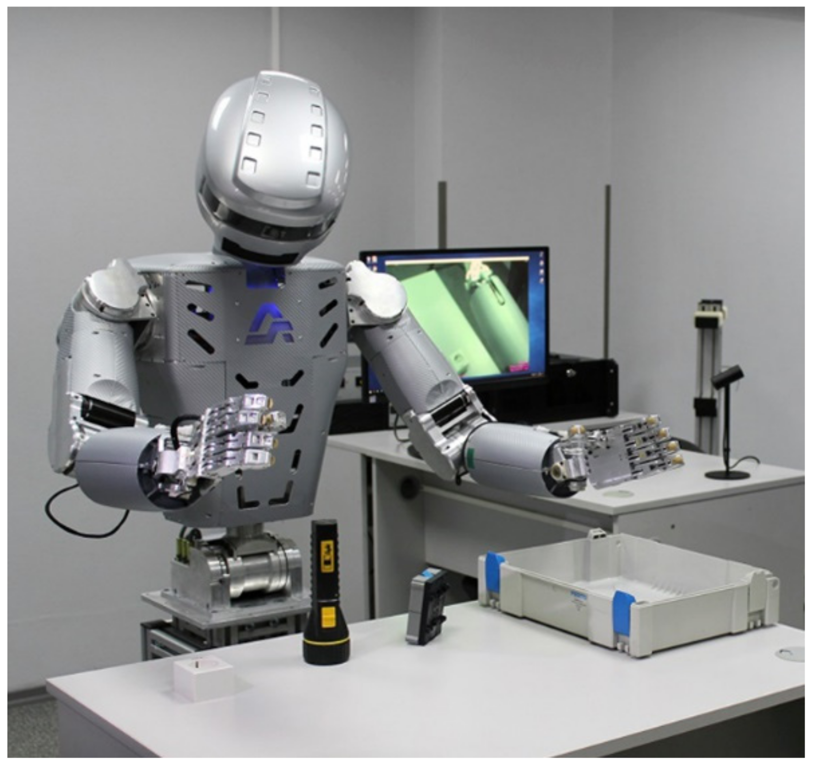
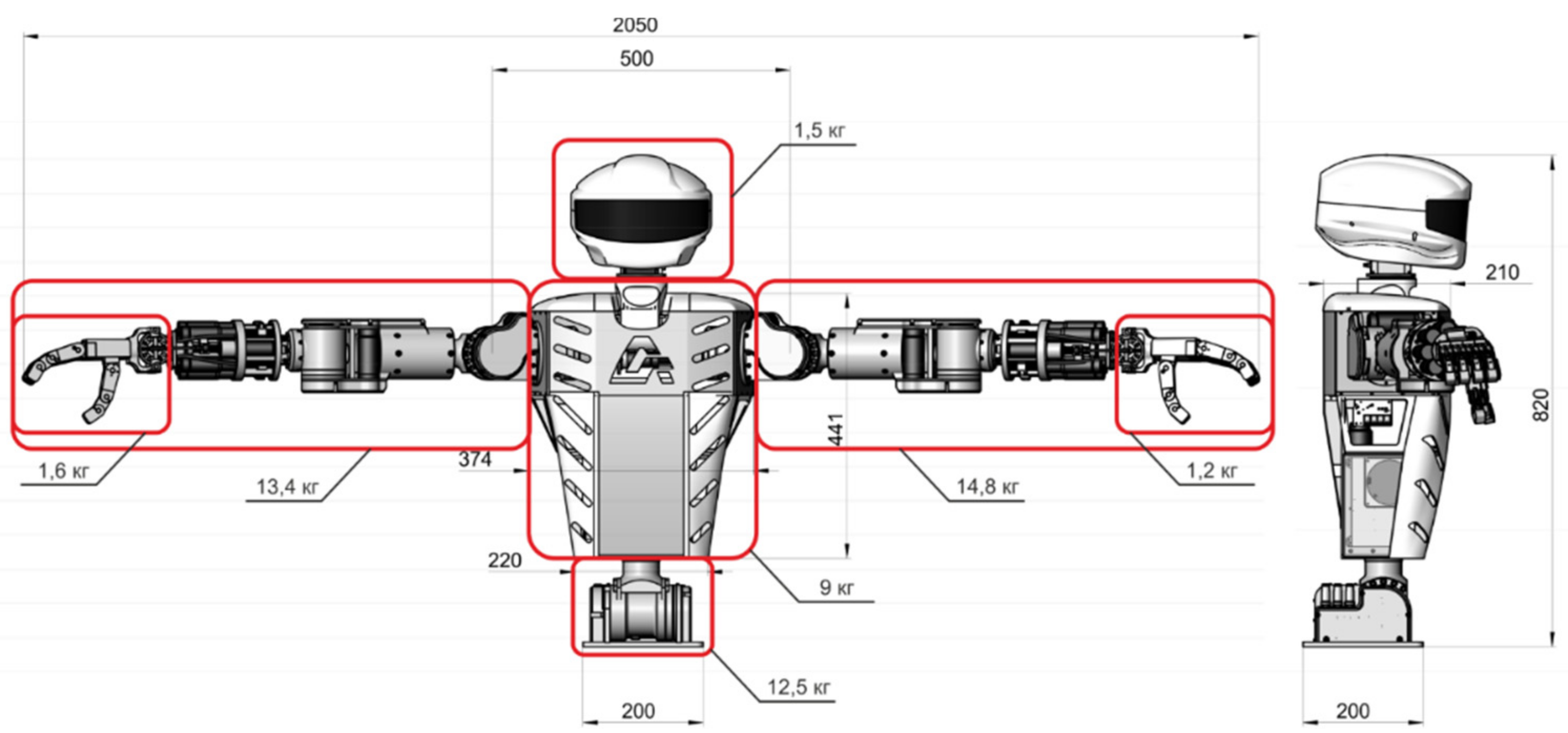
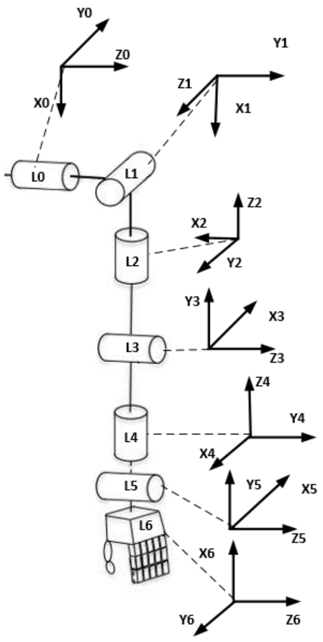
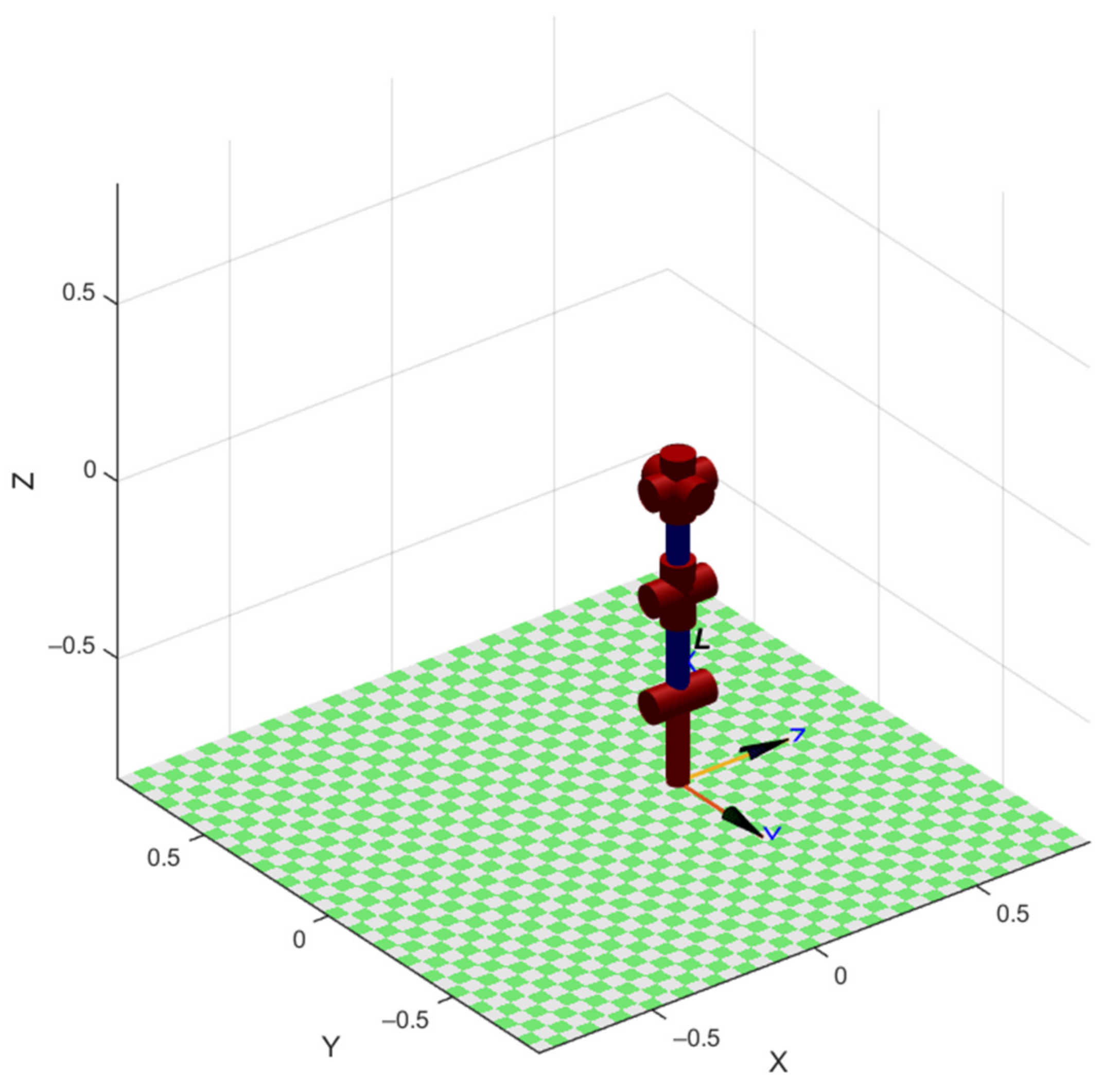
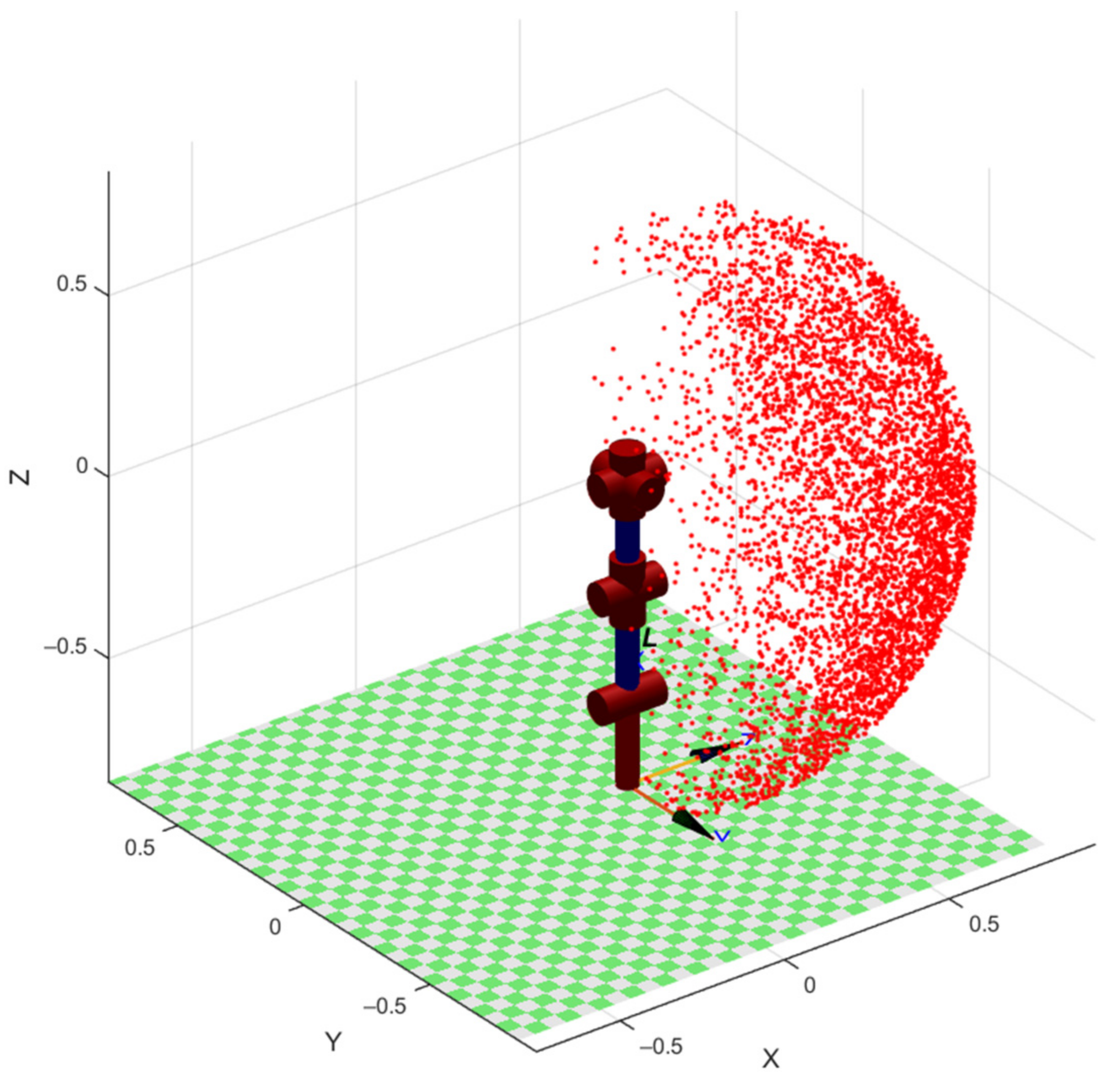
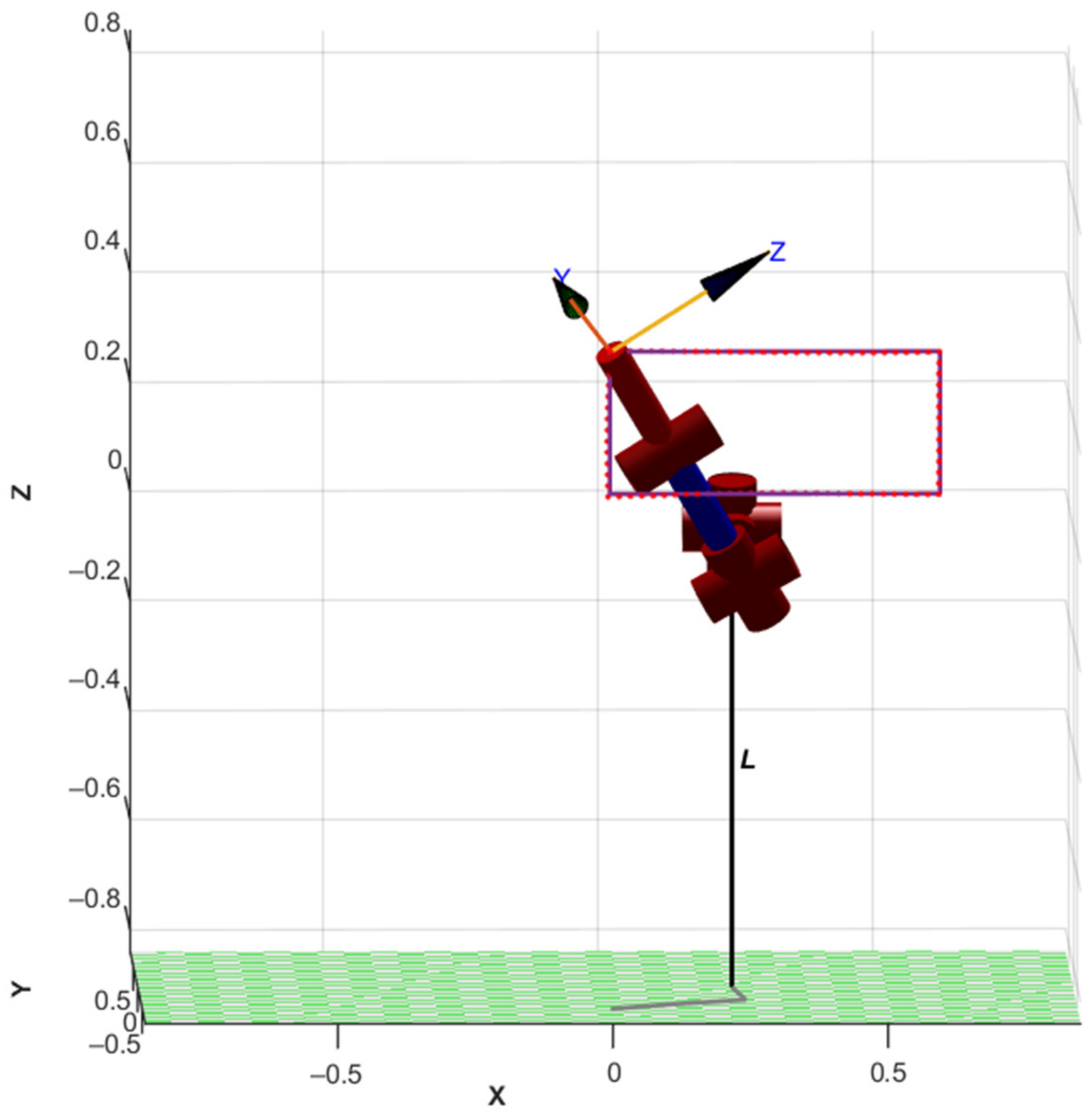
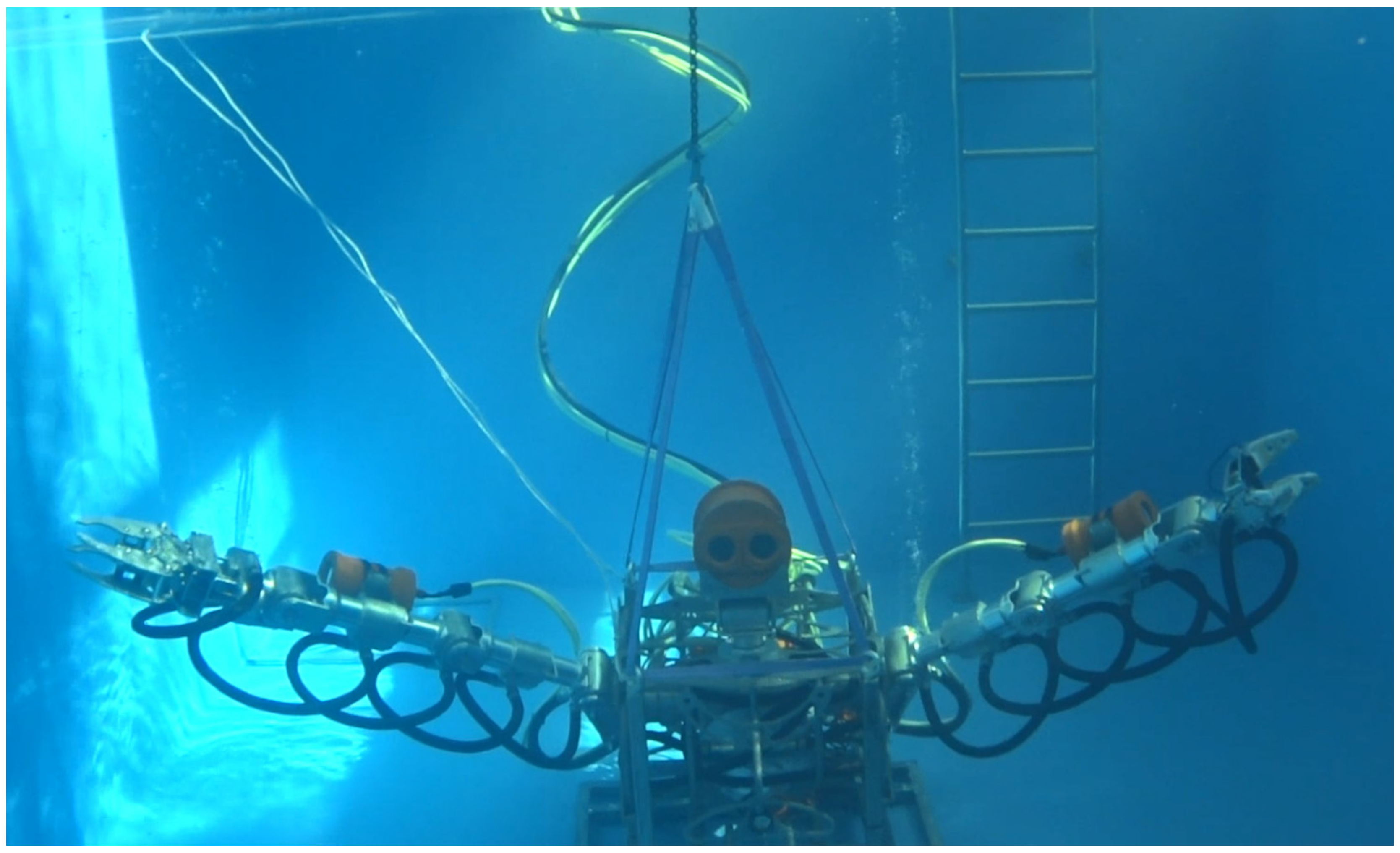
2.1. Kinematics Analysis of the Robot SAR-401
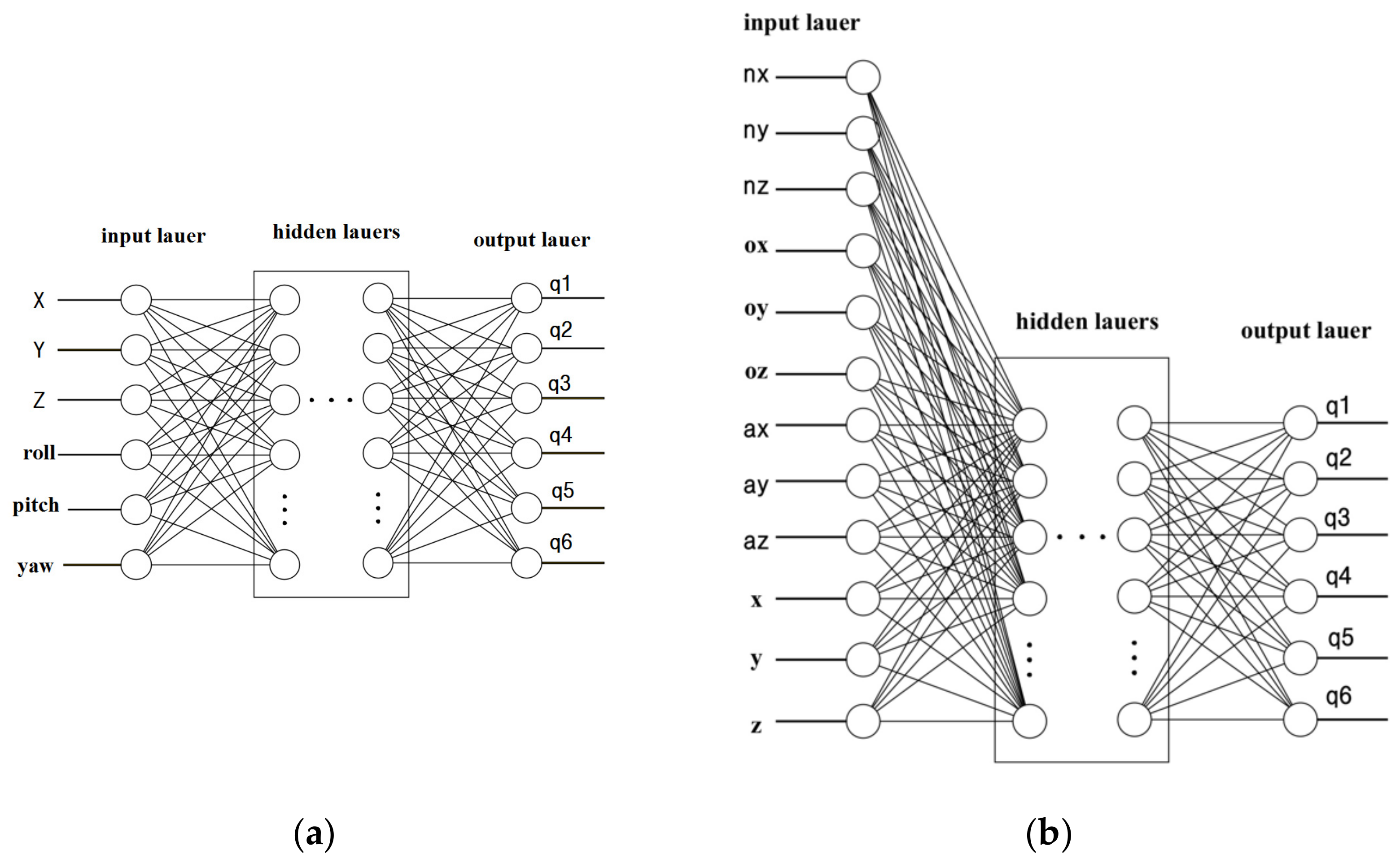
2.2. Training Dataset for Neural Network
2.3. The Amount of Training Data
2.4. The Activation Function
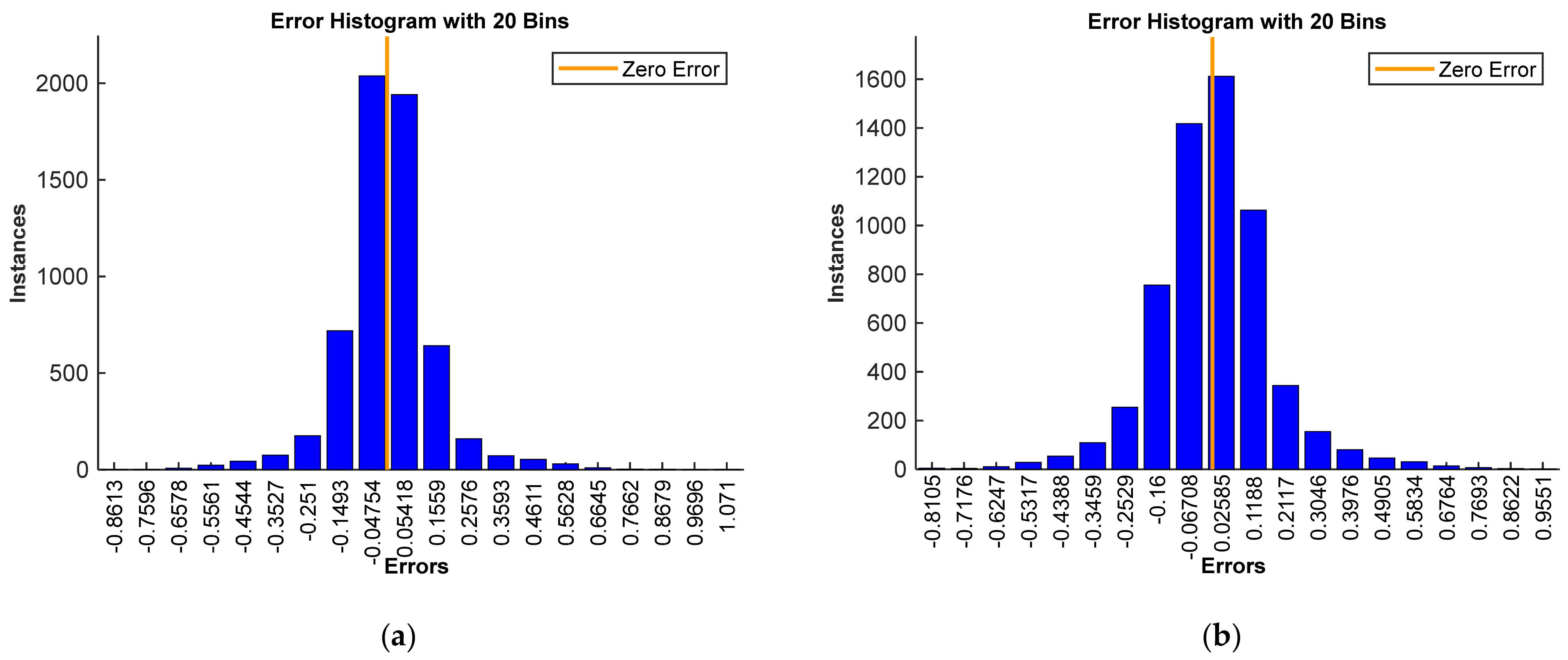
2.5. The Loss Function
2.6. The Learning Functions
- Levenberg–Marquardt (trainlm);
- Bayesian regularization backpropagation (trainbr);
- scaled conjugate backpropagation gradient (trainscg);
- resilient backpropagation (trainrp).
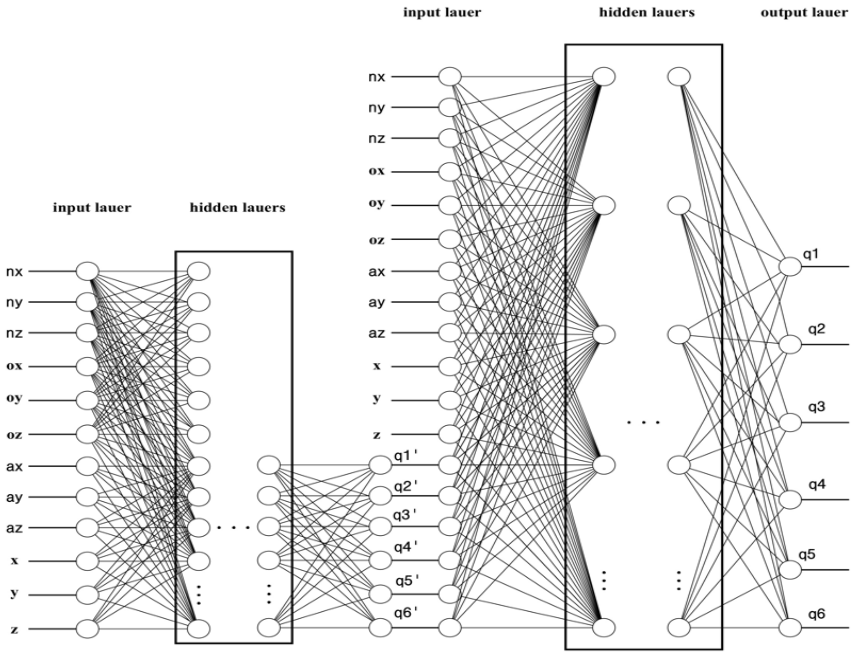
2.7. The Hidden Layers
- if there is only one output node in the neural network, and it is assumed that the required input–output connection is quite simple, then at the initial stage the dimension of the hidden layer is assumed to be 2/3 of the dimension of the input layer;
- if the neural network has several output nodes or it is assumed that the required input–output relationship is complex, the dimension of the hidden layer is taken equal to the sum of the input dimension plus the output dimension (but it must remain less than twice the input dimension).
- if in the neural network the required input–output connection is extremely complex, then the dimension of the hidden layer is set equal to one less than twice the input dimension.
- Based on the above recommendations, we will set the configuration of the hidden layer:
- the number of hidden layers is one;
- the number of neurons in this layer is set to one less than twice the input dimension.
3. Results
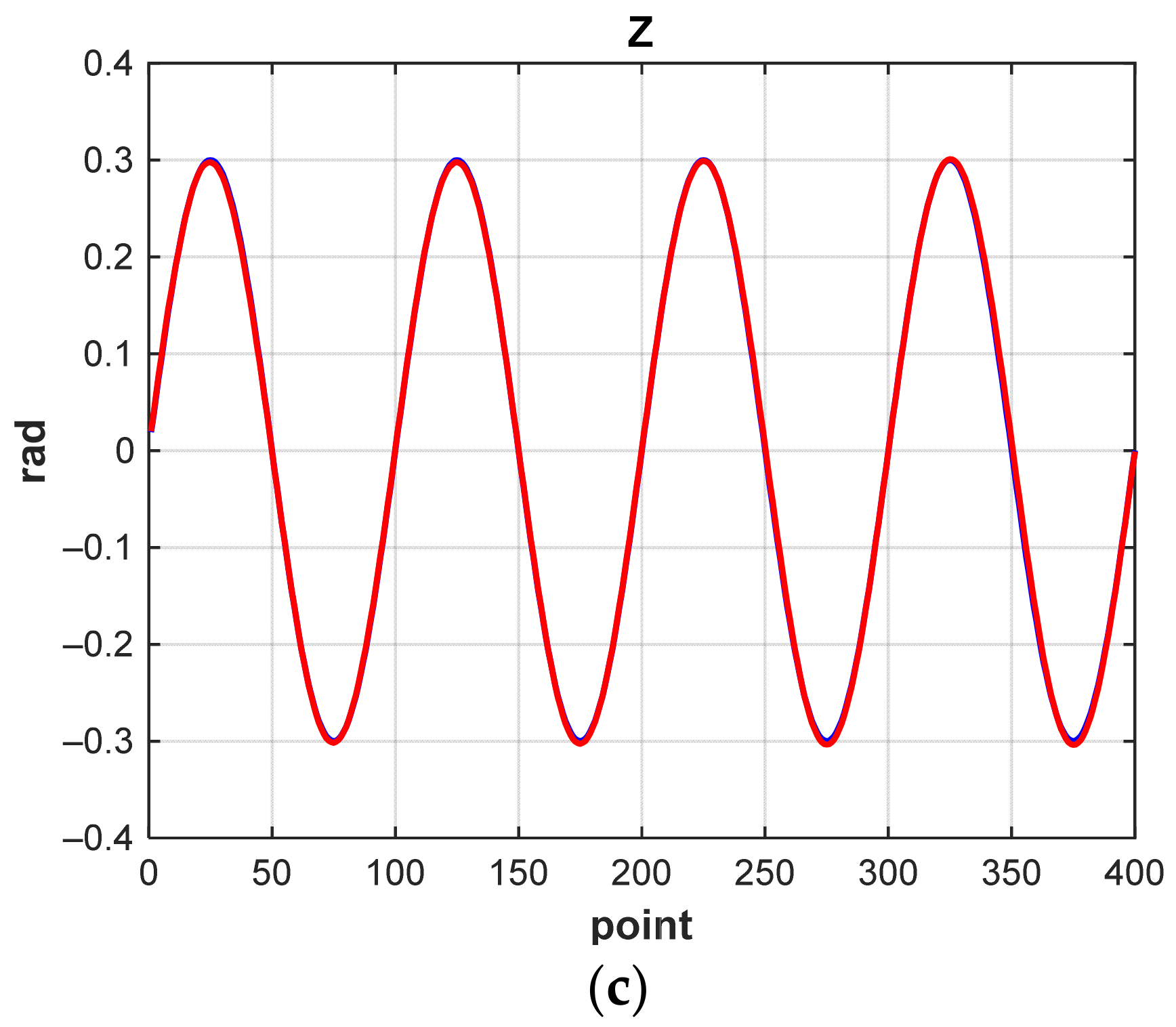
3.1. The “Correctional” Neural Network
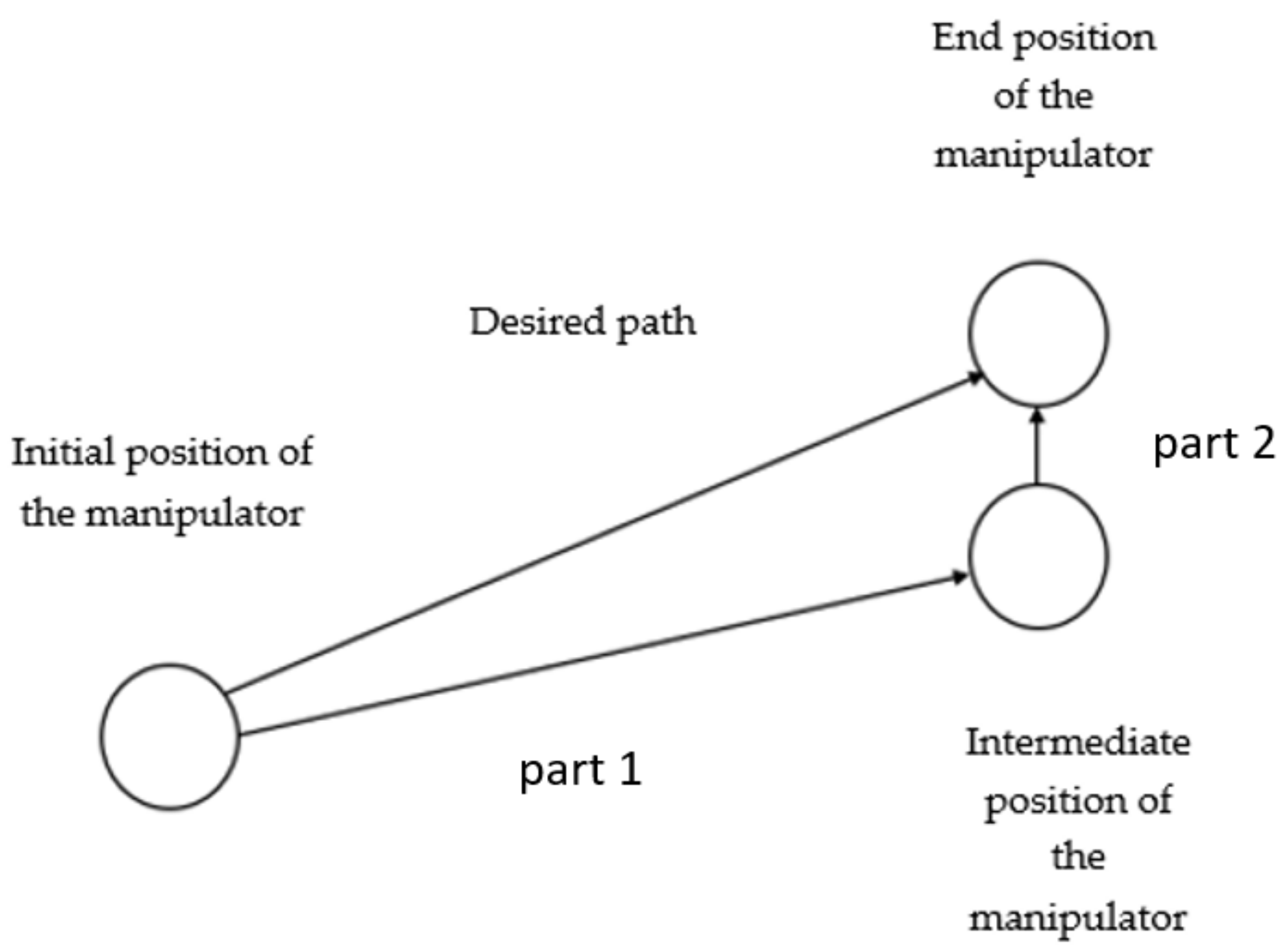
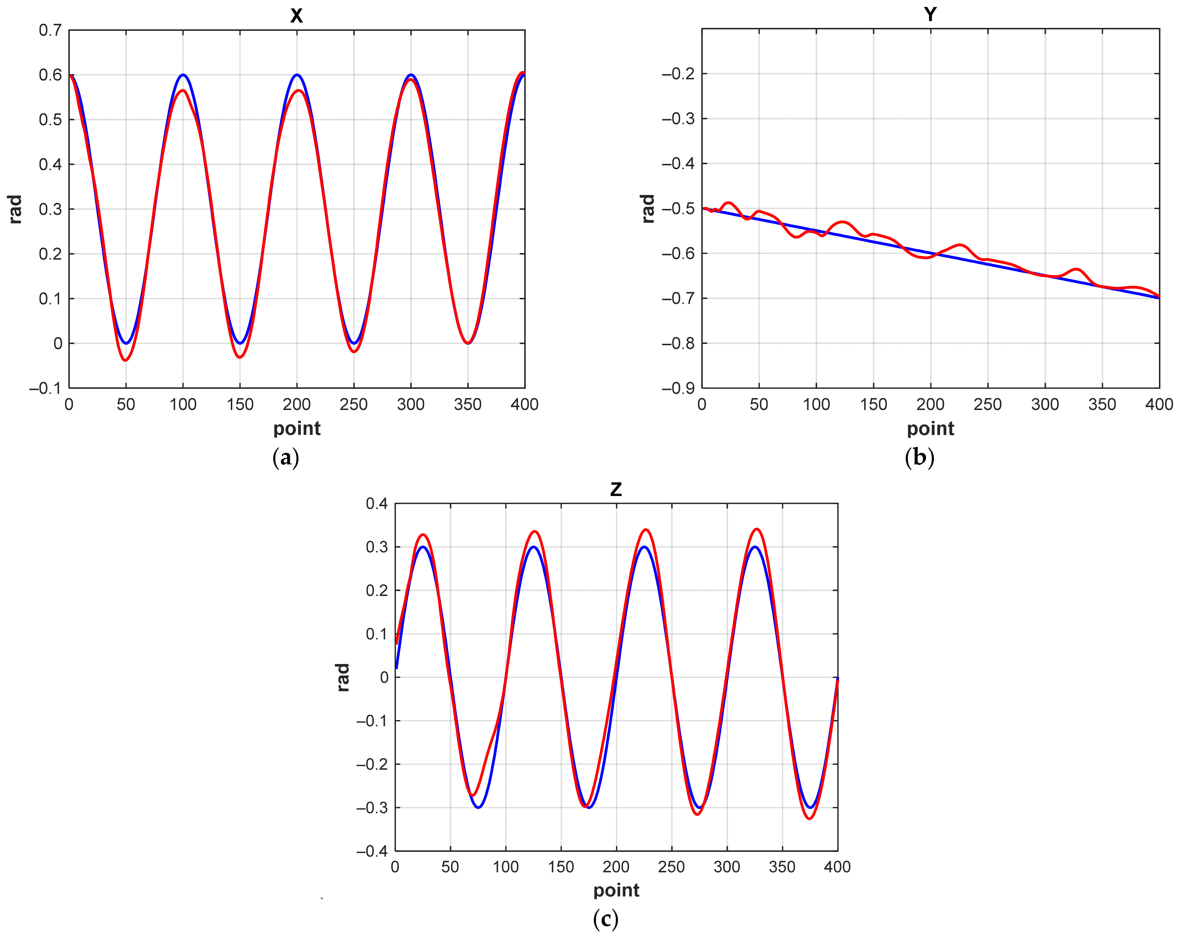
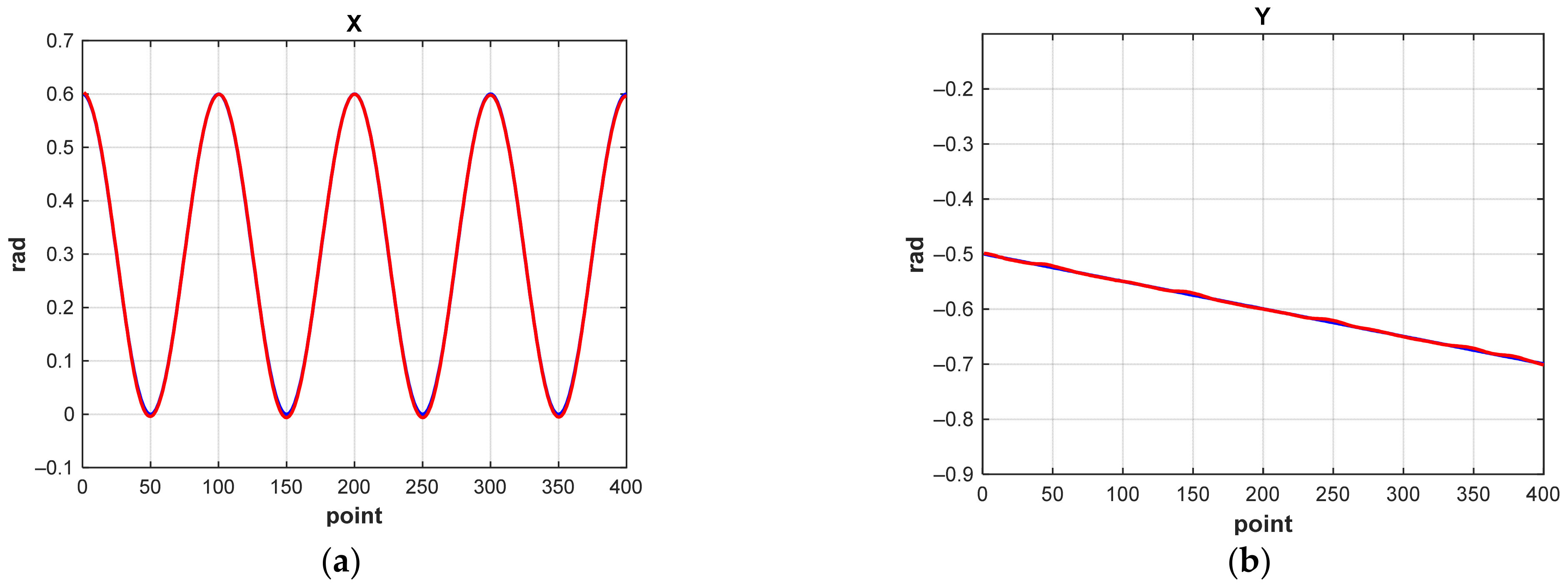
3.2. Example
4. Discussion
5. Conclusions
Author Contributions
Funding
Institutional Review Board Statement
Informed Consent Statement
Data Availability Statement
Conflicts of Interest
References
- Li, S.; Zhang, Y.; Jin, L. Kinematic control of redundant manipulators using neural networks. IEEE Trans. Neural Netw. Learn. Syst. 2017, 28, 2243–2254. [Google Scholar] [CrossRef] [PubMed]
- Hollerbach, J.; Suh, K. Redundancy resolution of manipulators through torque optimization. IEEE J. Robot. Automat. 1987, 3, 308–316. [Google Scholar] [CrossRef] [Green Version]
- Ahmed, R.J.; Almusawi, L.; Dülger, C.; Kapucu, S. A new artificial neural network approach in solving inverse kinematics of robotic arm (Denso VP6242). Comput. Intell. Neurosci. 2016, 2016, 5720163. [Google Scholar] [CrossRef] [Green Version]
- Bingul, Z.; Ertunc, H.M.; Oysu, C. Comparison Of Inverse Kinematics Solutions Using Neural Network for 6R robot Manipulator With Offset. In Proceedings of the ICSC Congress on Computational Intelligence Methods and Applications, Istanbul, Turkey, 15–17 December 2005; p. 5. [Google Scholar] [CrossRef]
- Xia, Y.; Wang, J. A dual neural network for kinematic control of redundant robot manipulators. IEEE Trans. Syst. Man Cybern. 2001, 31, 147–154. [Google Scholar] [CrossRef] [Green Version]
- Yang, Y.; Peng, G.; Wang, Y.; Zhang, H. A New Solution for Inverse Kinematics of 7-DOF Manipulator Based on Neural Network. In Proceedings of the IEEE International Conference on Automation and Logistics, Jinan, China, 18–21 August 2007. [Google Scholar] [CrossRef]
- Liu, J.; Wang, Y.; Li, B.; Ma, S. Neural network based kinematic control of the hyper-redundant snake-like manipulator. In Proceedings of the 4th International Symposium on Neural Networks, Nanjing, China, 3–7 June 2007. [Google Scholar] [CrossRef] [Green Version]
- Daya, B.; Khawandi, S.; Akoum, M. Applying neural network architecture for inverse kinematics problem in robotics. J. Softw. Eng. Appl. 2010, 3, 230–239. [Google Scholar] [CrossRef] [Green Version]
- Driscoll, J.A. Comparison of Neural Network Architectures for The Modelling Of Robot Inverse Kinematics. In Proceedings of the 2000 IEEE SOUTHEASTCON, Nashville, TN, USA, 7–9 April 2000; pp. 44–51. [Google Scholar] [CrossRef]
- Choi, B.B.; Lawrence, C. Inverse Kinematics Problem in Robotics Using Neural Networks; NASA Technical Memorandum; Lewis Research Center: Cleveland, OH, USA, 1992; Volume 105869. [Google Scholar]
- Peters, J.; Lee, D.; Kober, J.; Nguyen-Tuong, D.; Bagnell, J.A.; Schaal, S. Chapter 15. Robot learning. In Handbook of Robotic; Springer International Publishing: Cham, Switzerland, 2016. [Google Scholar]
- Alchakov, V.; Kramar, V.; Larionenko, A. Basic approaches to programming by demonstration for an anthropomorphic robot. IOP Conf. Ser. Mater. Sci. Eng. 2020, 709, 022092. [Google Scholar] [CrossRef]
- Bogdanov, A.; Dudorov, E.; Permyakov, A.; Pronin, A.; Kutlubaev, I. Control System of a Manipulator of the Anthropomorphic Robot FEDOR. In Proceedings of the 2019 12th International Conference on Developments in eSystems Engineering (DeSE), Kazan, Russia, 7–10 October 2019; pp. 449–453. [Google Scholar] [CrossRef]
- Kramar, V.A.; Alchakov, V.V. The methodology of training an underwater robot control system for operator actions. J. Phys. Conf. Ser. 2020, 1661, 012116. [Google Scholar] [CrossRef]
- Kramar, V.; Kabanov, A.; Kramar, O.; Putin, A. Modeling and testing of control system for an underwater dual-arm robot. IOP Conf. Ser. Mater. Sci. Eng. 2020, 971, 042076. [Google Scholar] [CrossRef]
- Denavit, J.; Hartenberg, R.S. A kinematic notation for lower-pair mechanisms based on matrices. Trans. ASME J. Appl. Mech. 1955, 23, 215–221. [Google Scholar] [CrossRef]
- Corke, P.I. Robotics, Vision and Control Fundamental Algorithms in Matlab; Springer: Cham, Switzerland, 2017; p. 693. [Google Scholar] [CrossRef]
- Chen, D.; Cheng, X. Pattern Recognition and String Matching; Springer-Verlag: New York, NY, USA, 2002; p. 772. [Google Scholar] [CrossRef]
- Haykin, S. Neural Networks a Comprehensive Foundation, 2nd ed.; Prentice-Hall: Hoboken, NJ, USA, 1999; p. 842. [Google Scholar]
- Ng, A. Machine Learning Yearning; GitHub eBook (MIT Licensed): San Francisco, CA, USA, 2018; p. 118. [Google Scholar]
- Szandała, T. Review and comparison of commonly used activation functions for deep neural networks. In Bio-Inspired Neurocomputing. Studies in Computational Intelligence; Bhoi, A., Mallick, P., Liu, C.M., Balas, V., Eds.; Springer: Singapore, 2021; pp. 203–224. [Google Scholar] [CrossRef]
- Rumelhart, D.; Hintont, G.; Williams, R. Learning representations by back-propagating errors. Nature 1986, 323, 533–536. [Google Scholar] [CrossRef]
- Nwankpa, C.E.; Ijomah, W.; Gachagan, A.; Marshall, S. Activation functions: Comparison of trends in practice and research for deep learning. In Proceedings of the 2nd International Conference on Computational Sciences and Technology, Jamshoro, Pakistan, 17–19 December 2020. [Google Scholar]
- Irwin, G.W.; Warwick, K.; Hunt, K.J. Neural network applications in control. IEE Control Eng. Ser. 1995, 53, 309. [Google Scholar]
- Heaton, J. Artificial Intelligence for Humans; Heaton Research, Incorporated: St. Louis, MO, USA, 2015; p. 374. [Google Scholar]
- Müller, B.; Reinhardt, J.; Strickland, M.T. Neural Networks: An Introduction; Springer: New York, NY, USA, 2012. [Google Scholar]


| Link, i | ||||
|---|---|---|---|---|
| 1 | 0 | π/2 | 0 | |
| 2 | 0 | π/2 | 0 | |
| 3 | 0 | π/2 | −0.3 | |
| 4 | 0 | π/2 | 0 | |
| 5 | 0 | π/2 | −0.3 | |
| 6 | −0.24 | 0 | 0 |
| Servo | Left Manipulator | Right Manipulator | ||
|---|---|---|---|---|
| Min | Max | Min | Max | |
| 0 | −90° | 0° | −90° | 0° |
| 1 | 0° | 105° | −105° | 0° |
| 2 | −40° | 40° | −40° | 40° |
| 3 | −110° | 5° | −110° | 5° |
| 4 | −40° | 40° | −40° | 40° |
| 5 | −10° | 10° | −10° | 10° |
| Algorithm | The Mathematical Expectation of Error (m) |
|---|---|
| trainlm | 0.0786 |
| trainbr | 0.0852 |
| trainscg | 0.1242 |
| trainrp | 0.1045 |
| Experiment N | Amount of Training Data | Number of Hidden Layers | Number of Neurons in Hidden Layers | Loss Function (m) | |
|---|---|---|---|---|---|
| RPY NN | MATRIX NN | ||||
| 1 | 40,000 | 1 | (11-RPY) (23-MATRIX) | 0.0836 | 0.0384 |
| 2 | 40,000 | 2 | [20,30] | 0.0259 | 0.0166 |
| 3 | 40,000 | 4 | [30,30,60,60] | 0.0119 | 0.0110 |
| 4 | 160,000 | 4 | [30,30,60,60] | 0.0094 | 0.0068 |
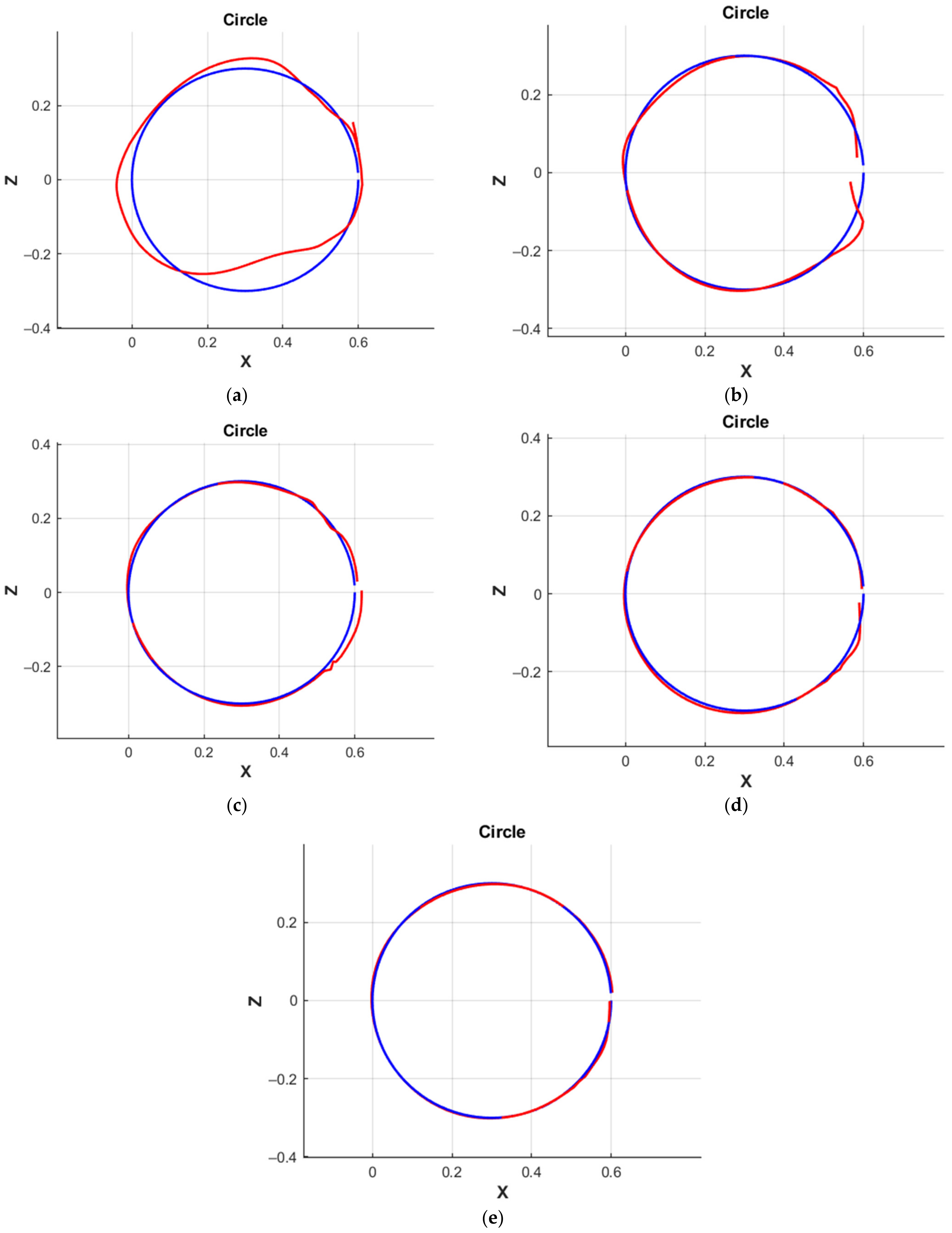
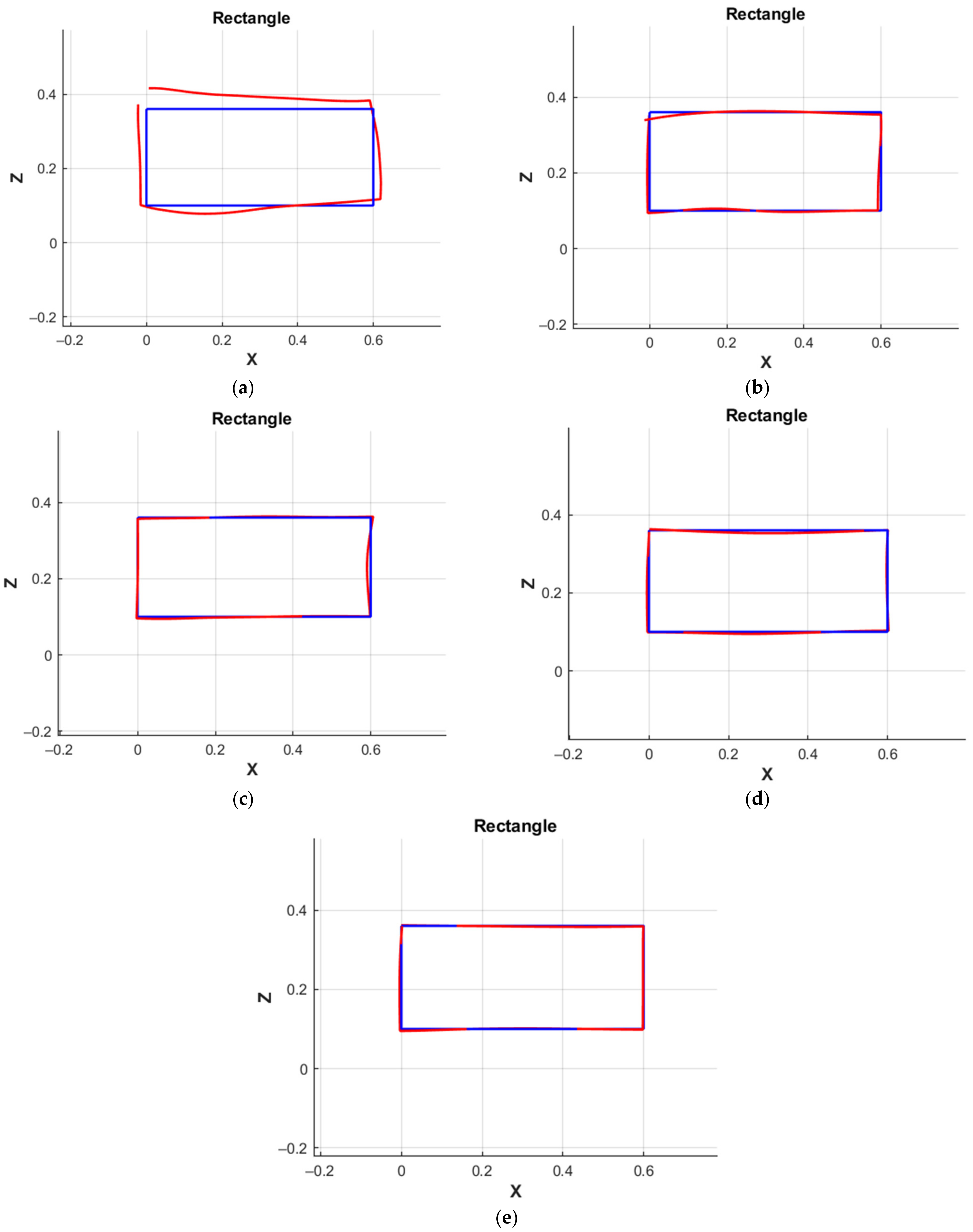
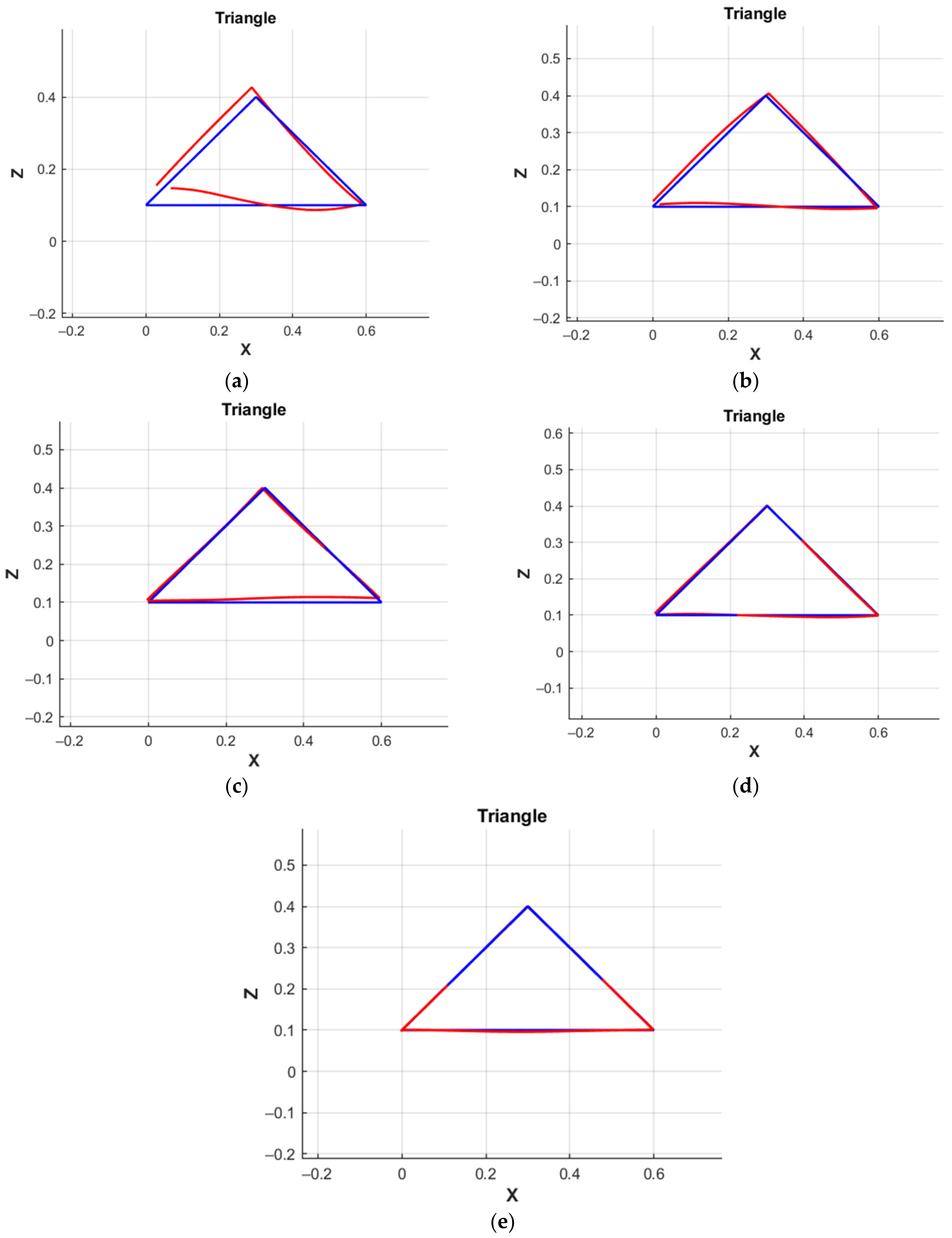
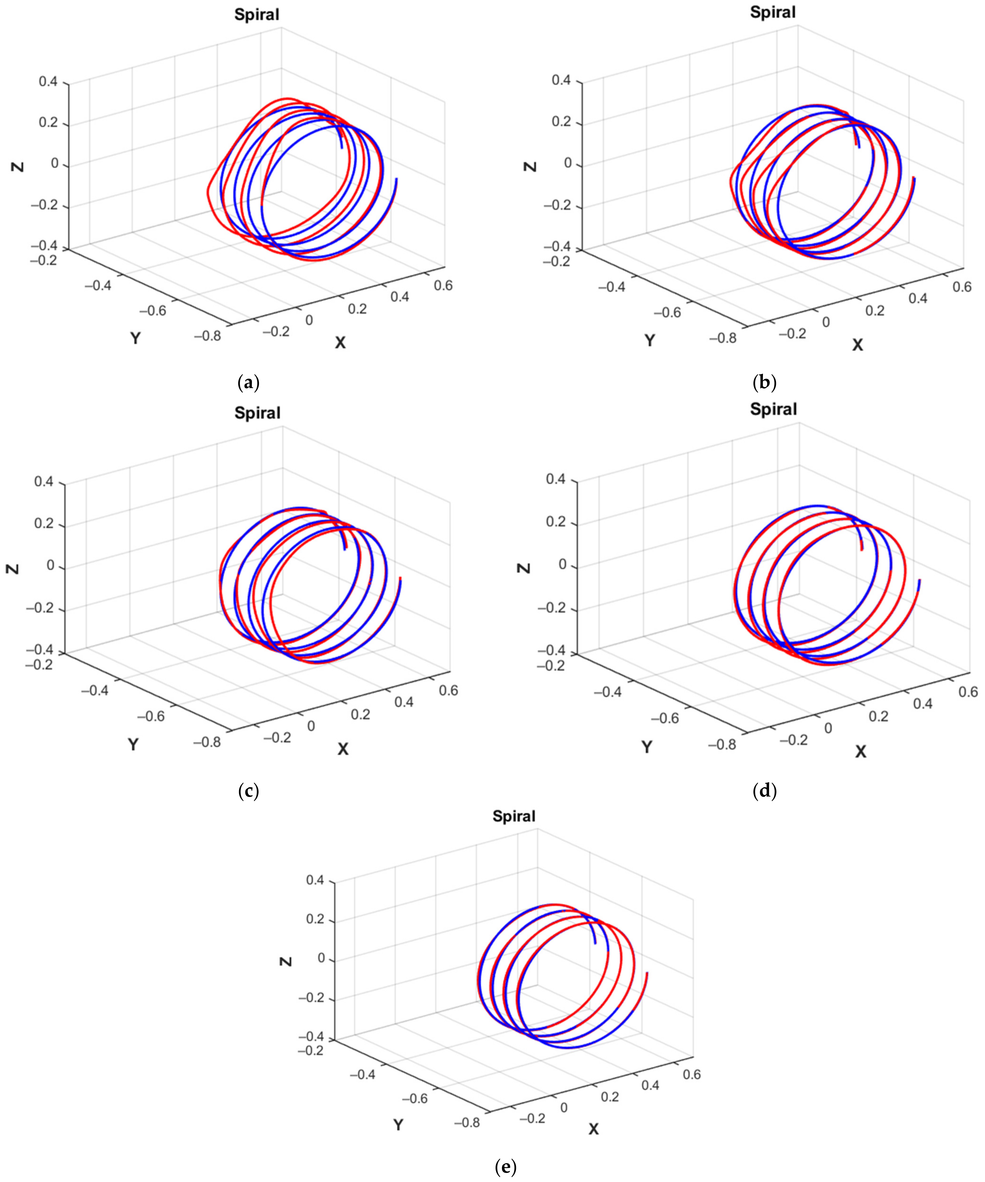
| Neural Network | Amount of Training Data | Number of Hidden Layers | Number of Neurons in Hidden Layers | Calculation Accuracy (m) | |||
|---|---|---|---|---|---|---|---|
| Spiral | Triangle | Rectangle | Circle | ||||
| MATRIX NN 1 | 40,000 | 1 | 23 | 0.0347 | 0.0358 | 0.0342 | 0.0483 |
| MATRIX NN 2 | 40,000 | 2 | [20,30] | 0.0168 | 0.0162 | 0.0094 | 0.0156 |
| MATRIX NN 3 | 40,000 | 4 | [30,30,60,60] | 0.0138 | 0.0077 | 0.0053 | 0.0112 |
| MATRIX NN 4 | 160,000 | 4 | [30,30,60,60] | 0.0068 | 0.0043 | 0.0042 | 0.0070 |
| The correctional NN | 160,000 | 4 4 | [30,30,60,60] [30,30,60,60] | 0.0035 | 0.0021 | 0.0032 | 0.0035 |
Publisher’s Note: MDPI stays neutral with regard to jurisdictional claims in published maps and institutional affiliations. |
© 2022 by the authors. Licensee MDPI, Basel, Switzerland. This article is an open access article distributed under the terms and conditions of the Creative Commons Attribution (CC BY) license (https://creativecommons.org/licenses/by/4.0/).
Share and Cite
Kramar, V.; Kramar, O.; Kabanov, A. An Artificial Neural Network Approach for Solving Inverse Kinematics Problem for an Anthropomorphic Manipulator of Robot SAR-401. Machines 2022, 10, 241. https://doi.org/10.3390/machines10040241
Kramar V, Kramar O, Kabanov A. An Artificial Neural Network Approach for Solving Inverse Kinematics Problem for an Anthropomorphic Manipulator of Robot SAR-401. Machines. 2022; 10(4):241. https://doi.org/10.3390/machines10040241
Chicago/Turabian StyleKramar, Vadim, Oleg Kramar, and Aleksey Kabanov. 2022. "An Artificial Neural Network Approach for Solving Inverse Kinematics Problem for an Anthropomorphic Manipulator of Robot SAR-401" Machines 10, no. 4: 241. https://doi.org/10.3390/machines10040241
APA StyleKramar, V., Kramar, O., & Kabanov, A. (2022). An Artificial Neural Network Approach for Solving Inverse Kinematics Problem for an Anthropomorphic Manipulator of Robot SAR-401. Machines, 10(4), 241. https://doi.org/10.3390/machines10040241