Article

Simulation of Static Tyre–Pavement Interaction Using Two FE Models of Different Complexity

1
Jozsef Cziraki Doctoral School of Wood Sciences and Technologies, University of Sopron, 9400 Sopron, Hungary
2
Department of Highway and Railway Engineering, Budapest University of Technology and Economics, 1111 Budapest, Hungary
*
Author to whom correspondence should be addressed.
Appl. Sci. 2022, 12(5), 2388; https://doi.org/10.3390/app12052388
Submission received: 31 January 2022 / Revised: 17 February 2022 / Accepted: 22 February 2022 / Published: 25 February 2022
(This article belongs to the Special Issue Road Materials and Sustainable Pavement Design)

Abstract

:
The aim of this research study was to analyse the approaches for establishing a spatial model of a radial truck tyre, based on the finite element method, in order to perform a realistic analysis of static as well as dynamic tyre–pavement interactions. A complex rubber tyre model having a large number of elements was formulated combining current state-of-the-art modelling techniques and, from that model, a simplified model having a smaller number of elements was derived. The complex model proved to be useful only for static loading, because of its high computational demand, while the simplified model proved to be also suitable for dynamic modelling. The two tyre models having different numbers of elements were compared by analysing the contact areas and stresses. Our results indicate that the basic idea of not changing material characteristics while simplifying the model, rebuilding only the carcass using composite shell elements, did not prove to be a satisfactory direction. The results given by the simplified model do not describe the behaviour of the radial tyre well but, rather, describe the behaviour of the diagonal tyre, regarding contact areas and stresses. On the contrary, when analysing stresses and strains in the road pavement structure, the two finite element models provided similar results in practice. Based on our comparison calculations, applying the average contact pressure q at analysis points at a 5–8 cm depth, the contact behaviour of the finite element tyre model can be used in any elastic-layer theory-based software.

1. Introduction

The mechanical–empirical road pavement structure design systems consider the pavement structure as an elastic structure, applying the thin-layer theory or the elastic-layer theory [1].
In any design procedure, knowledge of the loads on the pavement as well as the contact surface for loading is required. In the beginning, methods based on the Boussinesq equations supposed that the loading force is either concentrated or linearly distributed on the total wheel width. In the wake of pneumatic tyres, the main assumption was a circular contact area with an evenly distributed loading. This assumption has been adopted for a long time, providing simple calculations; moreover, a solution to the partial differential equations of elastic layers for this case only has been elaborated.
Theoretical approaches have been later supplemented by experimental solutions of the problem; the contact area of rubber tyres was determined by moving wheels of different loads onto a painted film between paper sheets or by spraying sand around wheels. As a result of technological developments, solutions for the direct measurement of contact stresses have appeared, such as the “Vehicle–Road Surface Pressure Transducer Array” [2].
According to current knowledge, stresses in the pavement structure are substantially determined by the value and distribution of contact stresses. Some distress types can be explained by these stresses, such as top-to-bottom cracking [3]. Despite experimental results, the majority of present-day design procedures still consider the contact area of truck twin tyres as two ellipses or even two rectangles, usually substituted by a circular surface of identical area. The distributed loading, i.e., the contact pressure, is supposed to be equal to the inflation pressure of the rubber tyre as a good approximation.
The tyre–pavement interaction can be successfully analysed by the finite element method at the present level of computing technology, instead of expensive and time-consuming in situ or laboratory measurements. This topic is well documented in the former studies [4,5,6,7].
The results of computer simulations may indicate some observations that may help with choosing the parameters of simplified models to better represent the realistic circumstances and processes. The motivation behind these kinds of developments is that, sometimes, the reproduction of the results reported in scientific papers via the application of finite element models can be difficult because of the unavailability of certain software components; therefore, the comparison of different tyre models in the literature is not always possible. Consequently, a method that can simply characterise and numerically describe the contact behaviour of complex finite element rubber tyre models may provide a great advantage in the systematization of research results in this topic area.

1.1. Objectives

The primary aim of the present research work is to develop a complex spatial rubber tyre model, based on the finite element method, to perform a realistic analysis of static as well as dynamic tyre–pavement interactions. To lower the computational demand of the finite element tyre model, a simplified model having a smaller number of elements was developed. A further goal is to understand the consequences of the reduction in the complex tyre model. The assessment of the two tyre models having different numbers of elements and modelling techniques was based on the shape and size of the contact areas as well as on the value and distribution of contact stresses. A new method is here proposed, which is useful for considering the contact behaviour of the developed finite element tyre models in the calculations applying the elastic-layer theory, even without the finite element model itself. To achieve the objectives above, the following main tasks were performed:
  • The establishment of a realistic spatial finite element model of a radial truck tyre based on manufacturer and literature data;
  • The development of the spatial finite element simulation of tyre–pavement interactions;
  • The calculation of contact areas and stresses using the complex finite element radial tyre model;
  • The derivation of a simplified finite element tyre model based on the complex model, for the analysis of dynamic tyre–pavement interactions;
  • A comparison between the contact behaviours of the complex and simplified finite element models using an example of a flexible road pavement structure;
  • A recommendation for a simplified calculation method of the contact behaviour of finite element tyre models having different content and numbers of elements.
Finally, the finite element tyre models were evaluated from the point of view of the stresses and strains occurring in the road pavement structure, performing comparison calculations via design software based on the multi-layer flexible pavement theory.

1.2. The Scope of the Analysis

The main focus of our study is on the finite element modelling of up-to-date radial tyres supposing static loading conditions. For the basic materials composing the rubber tyre, linear elastic (Hooke), hyper elastic, and viscoelastic material models were applied. According to the results of former research works, the value and distribution of the stresses at the tyre–pavement contact interface are independent of the mechanical characteristics of the layers forming the pavement structure [4]. Consequently, the contact process of the tyre–pavement interaction was analysed using a characteristic Hungarian flexible road pavement structure type only, applying a linear elastic material model for all the layer types.

2. Theoretical Background

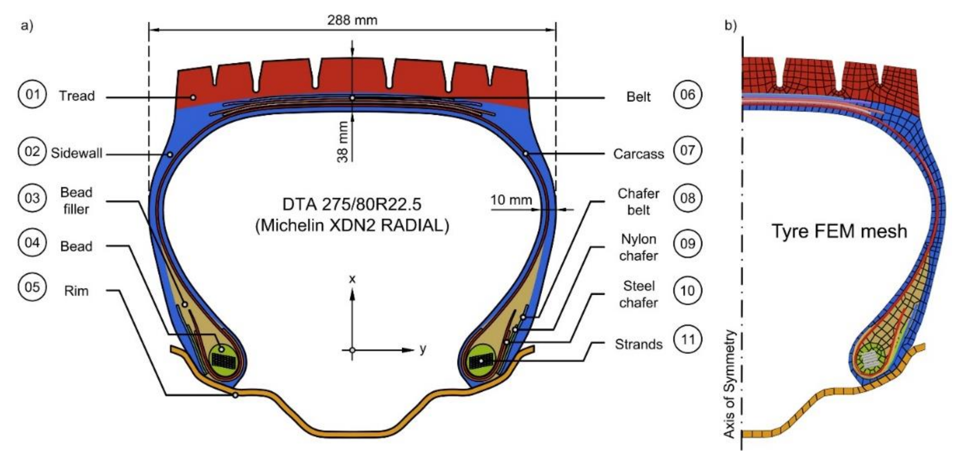
2.1. The Structure of the Rubber Tyre

Considering the interdisciplinary aspect of this research study, a brief review of the most important terms describing the structure of rubber tyres is here provided. While, for a common viewer, the tyre seems to be of a simple structure, in reality, an up-to-date tyre consists of about 10–20 different parts, providing, together, the required technical characteristics of the tyre. The most important parts of an up-to-date tyre are the following:
  • The tread is the part of the tyre that is in contact with the pavement; its task is to provide the cohesion, resistance to wear, and movement stability of the vehicle. Characteristically, it is made from synthetic and natural India rubber;
  • The belt is aimed at the reinforcement of the tyre, as it absorbs bumps and provides the optimal movement stability and rolling resistance to the vehicle. The belt is made from high-strength rubberized steel fibres; the position of the fibres is at ±10–30° in respect to the centre line, depending on the usage and the load bearing of the radial tyre;
  • The carcass provides the truss of the tyre; it keeps the shape of the tyre even in case of high inflation pressure and distributes the loading. It is made from rubberized rayon or polyester textile fibres;
  • The sidewall is made from natural rubber; it protects the carcass from sideways forces and transmits the momentum to the tread;
  • The filler helps to provide movement stability, steering, and comfort issues; it is made from synthetic rubber;
  • The chafer belt amplifies the movement stability and the steering accuracy; its material can be steel or nylon, resulting in different types of chafer belts;
  • The steel cord or strands provide stabilized nesting between the tyre and the body of the wheel; it is made from high-strength steel wires embedded in rubber. Depending on its manufacturing technology, the steel cord may include a bead.
The innermost layer of the tyre is airtight, its main task being to keep the inflation pressure and to prevent the infiltration of vapour and moisture.

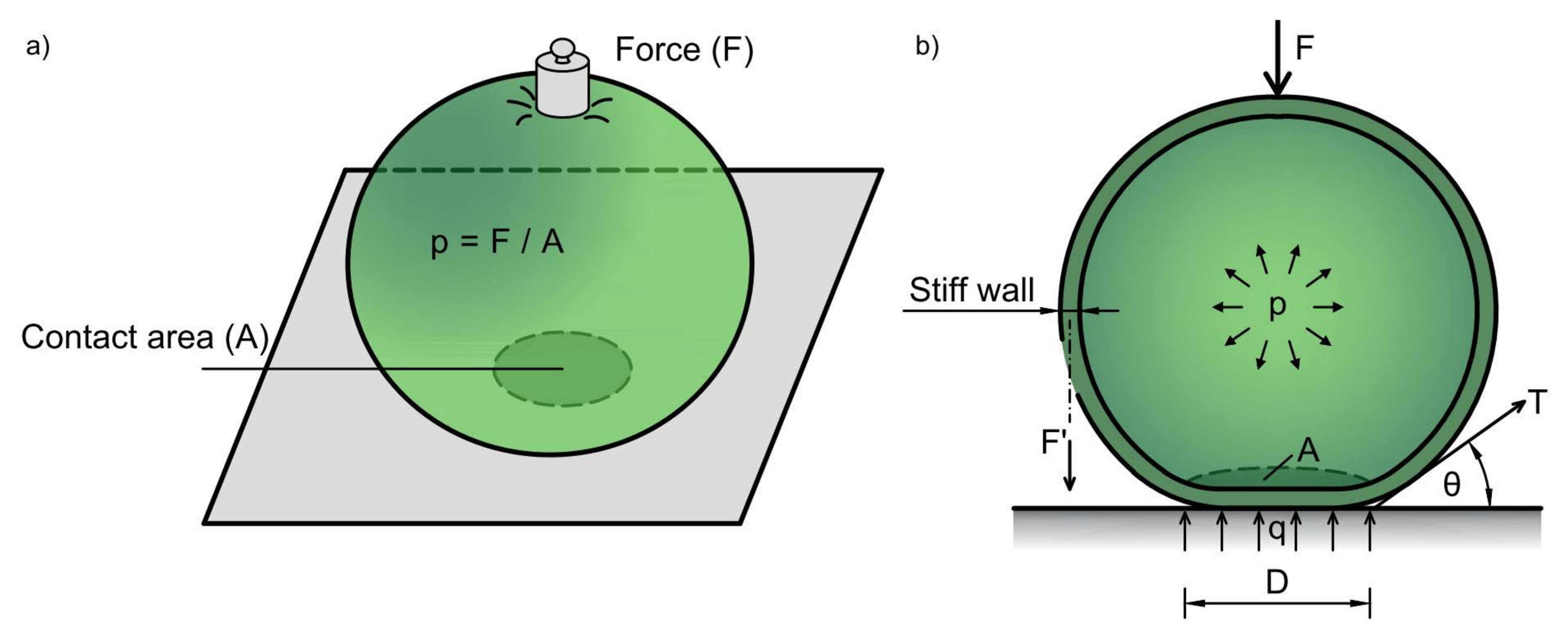
2.2. The Pressure Head of the Tyre

Vehicles stand on the pavement on their wheels. The wheel load is transmitted to the road pavement structure by the tyres. A plausible guess is that the F pressing force of the vehicle load is evenly distributed at the A contact surface area of the tyre:
p = F A ,
where p is the inflation pressure of the tyre, which is approximately equal to q , the specific contact pressure transmitted to the pavement by the tyre. Strictly speaking, the equality q p is true only in the case of an absolutely flexible tyre with no inner stiffness (Figure 1a). In case of a tyre that has an inner stiffness, the contact pressure can be higher or lower, even by 10–30%, than the inflation pressure of the tyre, according to the former literature (see, e.g., [8,9,10]).
These contradictory results have been explained by [11], who verified, by a physical consideration, that the specific contact pressure q of a balloon is, by necessity, lower than its inner air pressure p (Figure 1b):
q = p 4 T D sin θ + F A ,
where p is the inflation pressure, q is the contact pressure, T is the tensile force/unit of length (at the rim of the contact surface),   θ is the angle between horizontal plane and direction of force T , A is the contact circular surface, D is the diameter of the contact circular surface, and F is the load transmitted by the wall of the balloon.
Since the tensile force T depends on both the inner air pressure p and the external loading force F , the unknown average contact pressure q also depends on p and F ; therefore, generally, the following equation can be defined:
q = f 1 p + f 2 F , p ,
where f 1 p is the function of inflation pressure and f 2 F , p is the combined function of inflation pressure and load.
Van Vuuren extrapolated Equation (3), concerning balloons, to rubber tyres, where the physical structure of the tyre, its size, its tread type, the rubber toughness, and the wall thickness are introduced by a C factor [11] as follows:
q = f 1 p + f 2 F , p + C .
This theoretical function (4) was verified by [11] via laboratory measurements on an 8.25–20 × 10-ply rubber tyre:
q = 0.013 p + 10.5 F + 0.119 p + 125.9
in a generalised form,
q = a 1 p + a 2 F + b 1 p + C ,
where q and p are in kPa and the wheel load F is in kN. According to the empirical Equation (6), the contact pressure depends on the wheel load, inflation pressure of the tyre and, mainly, the C constant characterising the “flexibility” of the tyre. Similar relationships were provided by [11] for further tyre types and tested in the laboratory; their parameters can be found in Table 1.
The theoretical correlations can be verified by a finite element analysis. Among the most widely presently used finite element software is ABAQUS/CAE (Complete Abaqus Environment), which provides an efficient and complete solution for a wide range of industrial tasks. Leading tyre manufacturers, i.e., Hankook, started to utilise ABAQUS software at the beginning of the 2000s for developing modelling techniques that are in use today [12]; therefore, this software was chosen as suitable for our current research work.

3. Materials and Methods

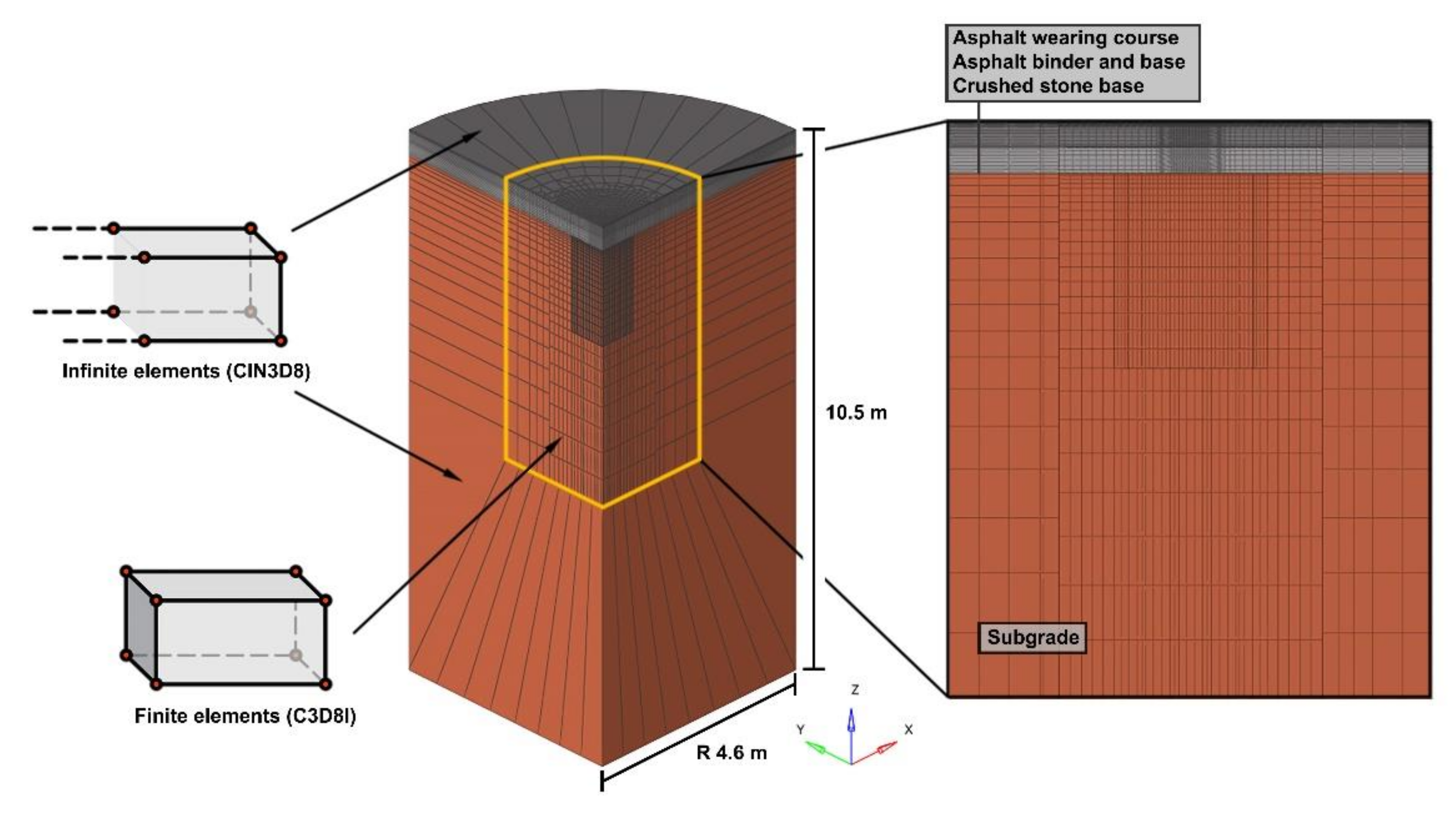
3.1. Finite Element Model of the Road Pavement Structure

The mechanical road pavement structure design is based on the theory reported in [13,14,15], modelling real road pavement structures as a flexible multi-layered system on a linear elastic, homogeneous, and isotropic half-space (multi-layer elastic analysis; MLEA). In this model, the mechanical behaviour of a layer of thickness h is given by the elastic or Young’s modulus E and the transverse contraction or Poisson’s ratio μ , according to Hooke’s law. Layers have absolute adhesion within the structure with no slipping at their boundaries. In addition to the MLEA theory, thanks to the work advanced in [16], finite element modelling has been implemented in the study of road pavement structures since the end of the 1960s because, among others, it allows one to consider the non-linear behaviour of materials.
A typical feature of the finite element method is that the infinite domains used in analytic solutions become finite. This feature is, sometimes, not reasonable, mainly in tasks including infinite or half-infinite continuums. In the case of road pavement structures, the problem occurs at the lowest layer, the subgrade, modelled as a homogeneous infinite half-space. The solution is provided by infinite finite elements, suitable for describing even infinite partial domains. Table 2 summarises the layer system and mechanical characteristics of the layers of the analysed road pavement structure.
The finite element model (Figure 2) prepared for this research study consisted of a cylindrical domain of the road pavement structure, where there were C3D8I (8-node linear) finite elements, surrounded, at the boundary in the radial direction, by CIN3D8 (8-node linear) infinite elements; additionally, at the bottom of the subgrade below, we considered there to be a transition into infinite elements (to control the size of the depression). In ABAQUS software, at the definition of infinite elements, the numbering of nodes needs to be considered, because only the first surface of an infinite element can be interconnected to the finite element mesh. Edges starting from boundaries head toward the direction considered as infinite and are located around a pole. According to the theory, the solution for the infinite space is approximated along these edges, while the elongations of these edges within the boundary meet in a pole.
Consequently, the proper positioning of nodes in the infinite direction is important, as their distance from the pole is two-fold, compared to the nodes on the boundary. Radial infinite elements were directed to the rotation axis of the cylindrical pavement structure model, while infinite elements at the bottom of the subgrade met at the intersection of the contact area between the pavement surface and the tyre and rotation axis of the cylindrical pavement structure model.
In the vicinity of the contact surface between the tyre and the road pavement, the elements had a 6-mm edge length, while, moving from the analysed area to the boundary, the mesh was coarser, up to a 100-mm edge length. The transition from fine to coarse areas of the mesh was modelled by a linear tied contact, since, in the elements of the coarse area, a high-stress gradient was not expected. This simple solution provided a better-quality mesh and smaller running time. In all layers of the road pavement structure with finite thickness, the adequate mapping of bending stresses was provided by at least 5 elements, integrated in a non-reduced way. The layers could not slip at their boundaries; they were modelled as ideally tied to each other. In the model, the nodes of the spatial continuum elements had 3 displacement degrees of freedom (u1, u2, and u3), while the nodes of the infinite finite elements at the infinite direction were constrained at the bottom, along the z-axis and, at sides, along the x- and y-axes. The decline in stress anomalies stemming from the clamping was provided by infinite elements with elastic material characteristics at the given pavement structure layer; therefore, theoretically, the boundary conditions should not have caused a significant error in the simulation.
The number of continuum elements used for modelling the road pavement structure was 206,421 supplemented by 1740 infinite elements.

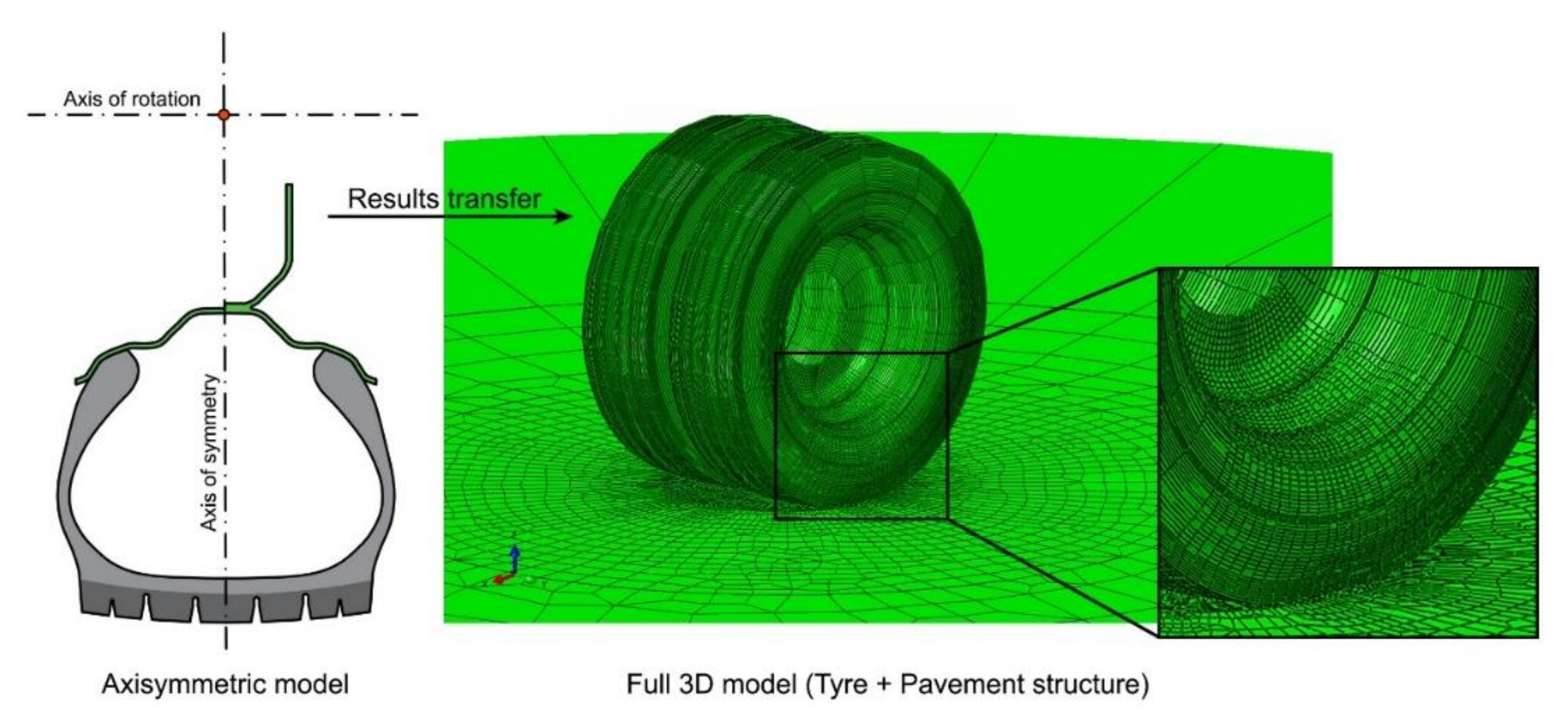
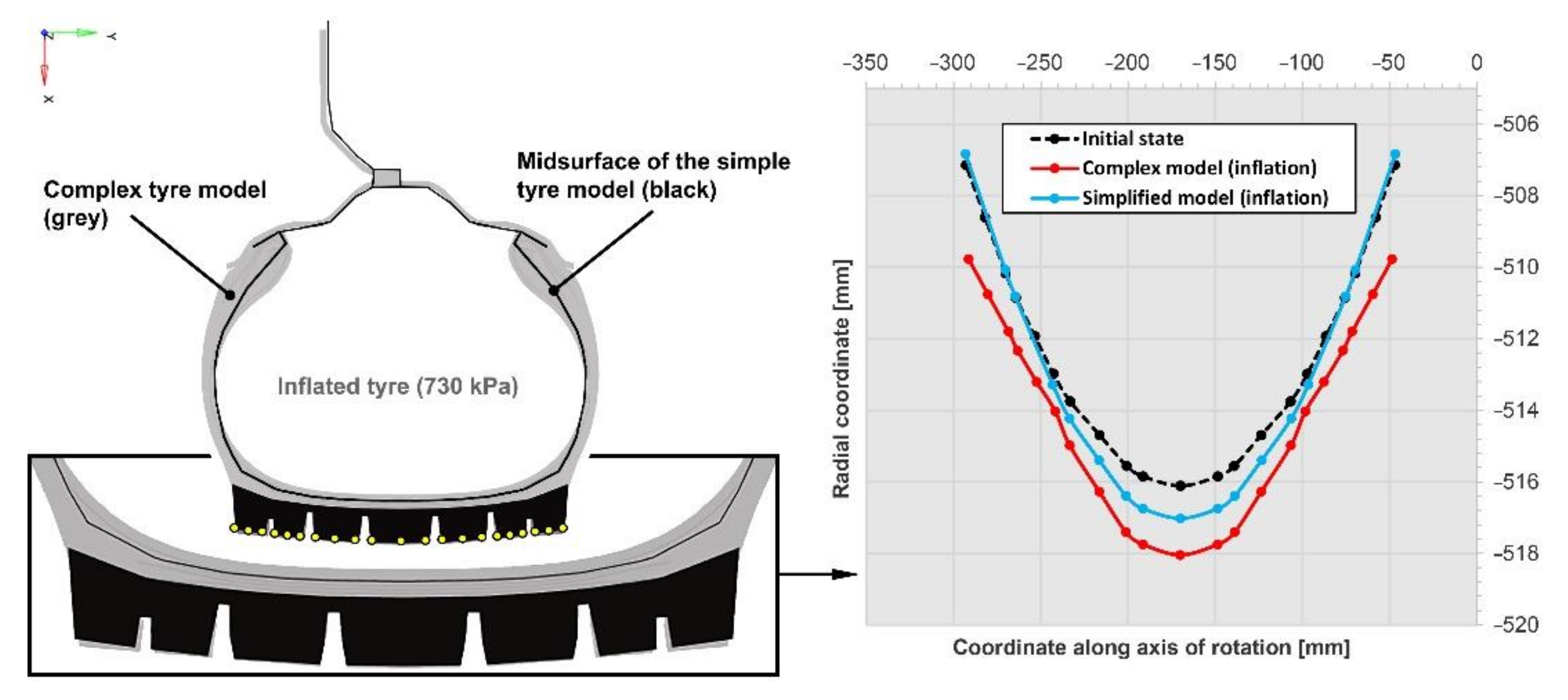
3.2. Complex Finite Element Model of the Rubber Tyre

The complex finite element model of the real rubber tyre was set up in two steps. In the first step, the pre-stress of the steel cord and the inflation pressure were formed, based on a planar axial symmetric model. In the second step, the 3D spatial tyre model in its equilibrium state was derived from the 2D model. These steps are described in detail in the next subsections.

3.2.1. The 2D Axial Symmetric Model

The finite element analysis (at the fulfilment of certain conditions) provides a possibility for a planar analysis of 3D bodies, resulting in significant reductions in the required computational time, space, and hardware capacity. For the modelling of the inflation of the tyre and its stretching to the body of the wheel disk, it is sufficient to solve a planar axial symmetric problem, meaning that only the radial cross-section of the tyre has to be modelled. The geometry of the structure of the tyre was reconstructed based on the cross-section drawing of the DTA 275/80R22.5-type tyre published by [5] (p. 21), with the overall width of the tyres being 288 mm and the dual spacing of the tyres being 315 mm.
The composite structure of the tyre is illustrated in Figure 3, the geometric values are presented in Table 3, and the material parameters are collected in Table 4, based on a literature review. The material parameters, as Yeoh’s hyper elastic, viscoelastic, and rebar, were collected from the works of [17,18]. The experimental determination of the material parameters of the tyre has been well summarised by [19].
The ABAQUS software prescribes the position of the cylindrical co-ordinate system, required to the definition of the axial symmetrical problem, where the x-axis is the radial axis, and the y-axis coincides with the z-axis. According to this, the cross-sectional model of the tyre is defined on the xy-plane (Figure 3b). In ABAQUS software, there is no need for special commands to define the axial symmetric problem, but, necessarily, the mesh can be constructed only from axial symmetric elements. The following element types were used for the tyre model:
  • CAX4 (4-node bilinear continuum element) for linear elastic or elastic–plastic materials;
  • CAX4H (4-node bilinear hybrid continuum element) for hyper elastic materials;
  • SFMAX1 (2-node linear membrane-like surface element) for rebar.
Surface elements are, by their appearance, membrane elements with no thickness. They are usually applied for defining surplus weight or distributed loading on the surface, but they are also useful for the simplified consideration of the rebar of the tyre.
A great advantage of the SFMAX1 surface element is that the rebar has to be modelled only in the radial section, and the cross-section of the rebar can be given by parameters that are independent of the finite element mesh. A further advantage is that the surface elements do not need to join with nodes to the other elements of the finite element mesh; these can be defined as an embedded element. In the tyre model, the material of the rubber is the “host element” assigned to the rebar.
The clamping of the axial symmetric model is at the intersection of the axis of the rotation of the wheel and the axis of symmetry of the tyre (Figure 3b). Some degrees of freedom (DOFs) of the clamping point have to be constrained, namely, the 2 (U2) and the 6 (UR3) degrees of freedom, in order to obtain no displacement along the axis of rotation; moreover, the radial cross-section cannot turn around its plane.
The cross-section of the tyre model in Figure 3a reflects the state before the inflation and the nesting onto the body of the wheel. The interaction between the body of wheel and the tyre was worked out based on the tear analysis of the rebar published by [20].
At the beginning of the simulation, a tensile stress value of 30 MPa was given in the strands at a longitudinal direction, which provided a fine nesting of the tyre rim onto the body of the wheel. The tyre rim on the body of the wheel may slip during inflation (here, a friction coefficient of 0.3 was chosen); moreover, in case of a radical surplus pressure, the rim may even detach from the body of the wheel. At this point, it was already worth comparing the stresses in the tyre and the shape of the inflated tyre to the measurement results ([20,21]). Considering the further step of the tyre–pavement interaction simulation, here, in the axial symmetric model, the contact surface of the tread was already defined.

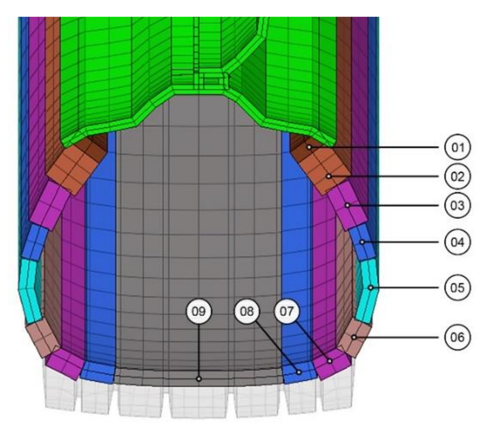
3.2.2. The 3D Full-Body Model

The 2D axial symmetric model of the rubber tyre is a simulation of a particularly quick run, despite the contact surfaces, which means a run time of less than one minute in a normal workstation (4 CPU with 3.5 GHz clock speed). A similar task in 3D requires several tens of minutes, even at unaltered performance. Nevertheless, for the next steps of the research study, where the interaction between the pavement and the tyre was analysed, it was indispensable to increase the complexity of the finite element model. ABAQUS software was able to generate a 3D model from the 2D axial symmetric model by applying the *SYMMETRIC MODELL GENERATION command, projecting the stress state of the axial symmetric model to the 3D mesh. After this projection, we had to perform a calculation called the equilibrium step in order to obtain a real equilibrium state of the projected stress state in the 3D model.
In the generation process for the 3D full-body model of the tyre, it was worth generating a finer mesh, at the parts where the tyre–pavement interaction was expected, while applying a coarser approximation for the other elements, in this way sparing the computational time and hardware performance (Figure 4). The CCL 12 cylindrical finite element was applied at the coarse mesh parts of the model, because these elements can better track the cambered spatial parts with their surplus nodes placed at the perimetrical direction. For modelling the contact surface, it is recommended to choose traditional elements in order to achieve the equilibrium state quicker during the solution. In the generation process for the 3D model, the node, element, and contact surface groups defined in the axial symmetric model developed automatically, which is why, already in the 2D model, the contact surfaces required for the tyre–pavement interaction were defined. At this step, it was necessary to input the road pavement structure model by applying the *INCLUDE command. It is advisable to place the mesh of the road pavement slightly far from the tyre mesh; thus, the two meshes remain initially distant. For the simulation of the tyre–pavement contact, the contact pairs and their interaction characteristics are given.
For the proper contact definition, the “softer” material, that is, the tread of the tyre, requires a finer meshing, and it can be chosen as the “slave” surface in the contact pair. Since, in this research study, only the static loading case was analysed, there was no need to define a complex friction model between the road pavement (the wearing course) and the tyre. Moreover, as observed by [24,25], the non-friction connection provides more realistic results. This observation is explained by the fact that, because of the friction effect, shear stresses and faults occur at the rim of the tread pattern of the tyre. This scenario does not occur in case of the rolling movement of the tyre, nor in case of the standing position derived from its rolling movement. The clamping of the tyre was at the same point in the 3D model, although all 6 degrees of freedom were constrained and the inflation pressure of the tyre was considered as a distributed load.

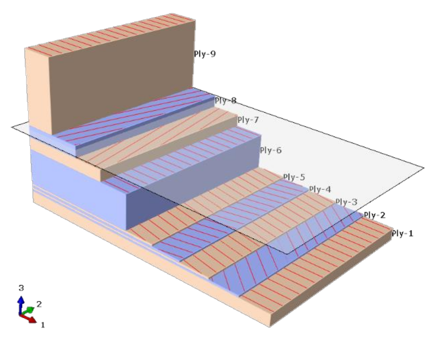
3.3. The Simplified Finite Element Model of the Rubber Tyre

Proceeding from the above-mentioned complex finite element model of the rubber tyre, another, by far more simplified tyre model was created. This simplified model is suitable not only for describing the load transition, but also for parametric analysis, since the complexity of the simulation and, consequently, the running time are significantly decreased. The following main points were taken into account at the stage of model definition:
  • Tyre stiffness: the load transition is possibly described at the proper accuracy in the model;
  • Parametric analysis: the preparation simulations (i.e., inflation) had to run quickly;
  • The structure of the FEM model: adjusting tyre parameters independently of the finite element mesh (i.e., thickness of the sidewall, composition of belts, etc.);
  • The model had to be suitable for explicit simulations, even as a rotating body, without corrupting the integration time.
The simplified tyre model consisted of a combination of shell and continuum elements, primarily modelled in 3D. For the complex geometry of the tread, reduced integration linear continuum elements (C3D8R) were chosen, while, for the other parts of the tyre model, reduced integration linear shell elements (S4R) were chosen. The connection between continuum and shell elements is a tied contact (*TIED), considering the shift of the middle surface of the shell elements and their thickness. The steel body of the wheel was modelled only by its middle surface, supposing an 8-mm wall thickness, and its material was considered as linear elastic, applying the standard parameters of structural steel.
The basic idea of the simplified tyre model is that it keeps all the realistic material parameters used for the complex model. The inner structure of the tyre, being the most complicated part requiring a lot of information, was redefined, applying composite layered structure shell elements of various materials, using the composite supplementary function of ABAQUS software. The shell elements, in this case, were grouped into 9 groups and the characteristics of each were defined specifically, describing the composition of the complex tyre as precisely as possible. The following material groups were distinguished in the layered structure:
  • Rubber sidewall: homogeneous, isotropic, hyper elastic rubber layer;
  • Rubber filler: homogeneous, isotropic, hyper elastic rubber layer;
  • Carcass: simplified, it is a homogeneous, orthotropic thin plate;
  • Steel cord: simplified, it is a tight steel ring in the composite layer;
  • Steel chafer: simplified, it is a homogeneous, orthotropic thin plate;
  • Belt layer: simplified, it is a homogeneous, orthotropic thin plate, where the grainline substantially influences the stiffness of the tread of the tyre.
In the case of a composite shell element, the material parameters and grainline were defined in a cylindrical coordinate system, assigned to the tyre model. Table 5 shows the layer structure of element groups, where the order of layers started from the inner wall of the tyre and advanced outwards. Figure 5 and Figure 6 illustrate the shell element groups and the layered structure. The tread out of continuum elements was associated with the material property of tread rubber (Table 4).
In Table 5, the isotropic materials that are reported had an angle of 0 degrees, since, in ABAQUS, it is obligatory to input the grainline for any composite shell element. The total thickness of the composite shell element is the sum of its layer thicknesses. The thicknesses of the rubber layer were collected from the cross-sectional drawing. The determination of the thicknesses of the carcass and the various belt layers proved to be difficult, because these are defined, in the composite shell element, as a thin, homogeneous, orthotropic plate, not as individual wire fibres. The determination of their thicknesses, therefore, was based on the moments of inertia, calculated from the cross-section. The composition, similar to the case of the complex model, was based on the cross-sectional drawing of the DTA 275/80R22.5-type tyre, published by [5].

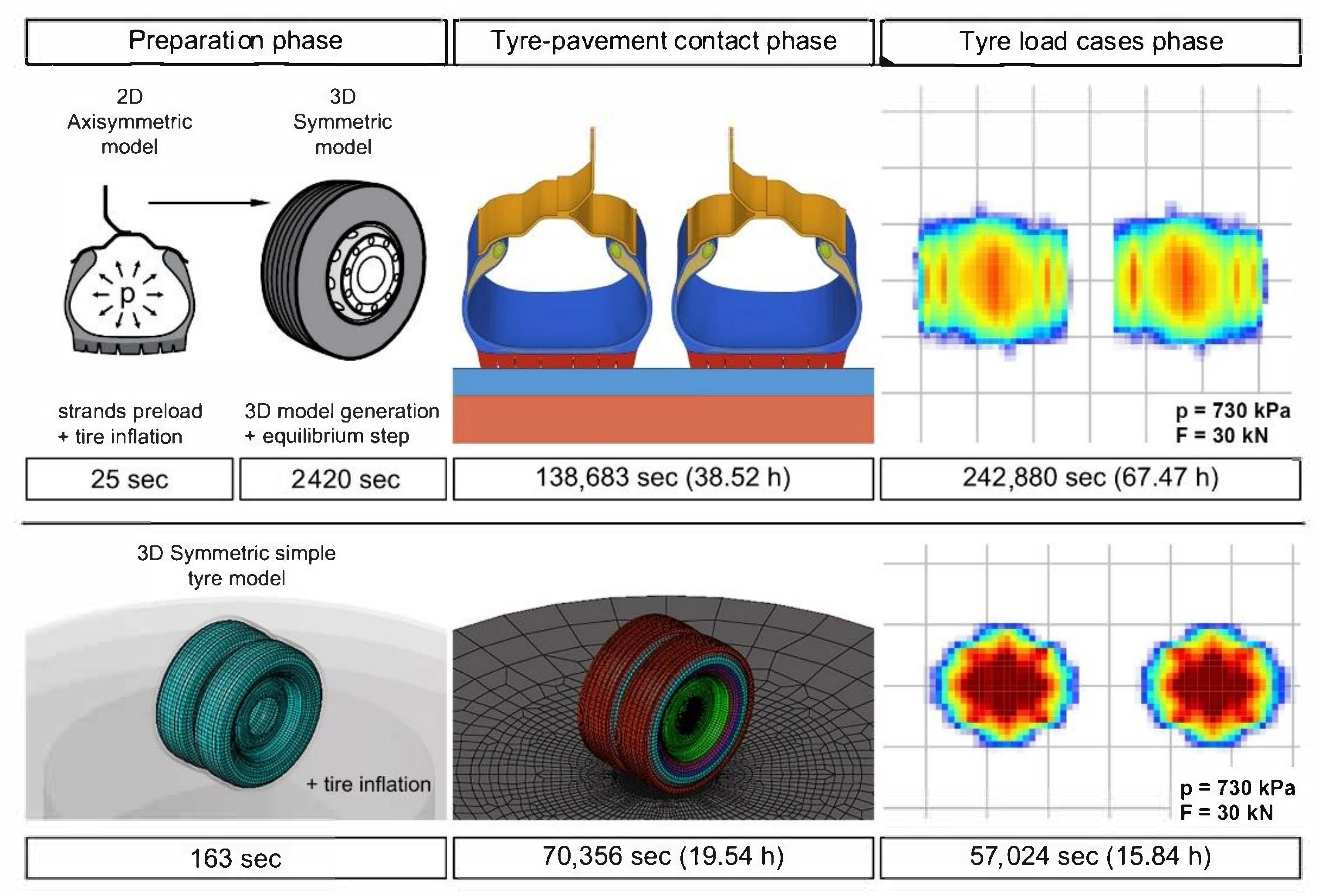
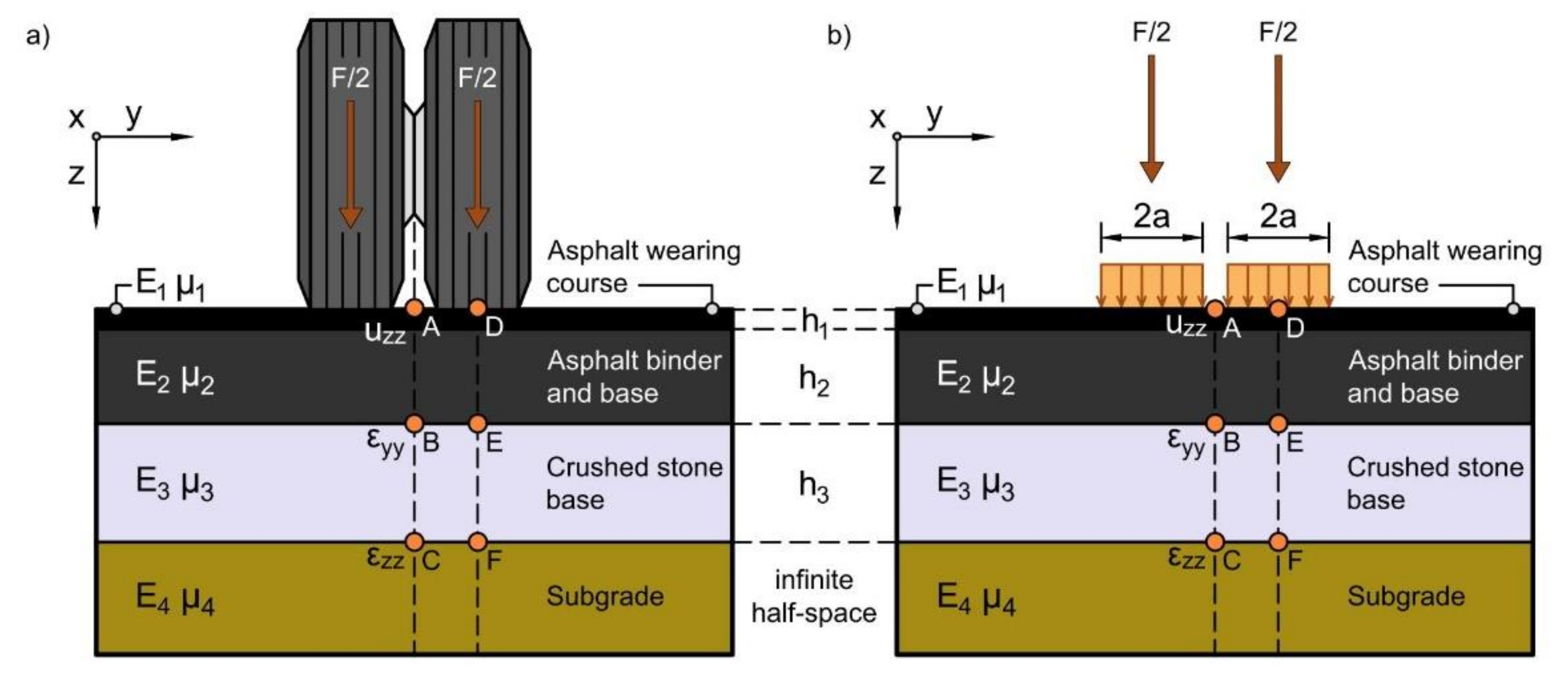
3.4. The Tyre–Pavement Interaction Simulation

The behaviour of the two kinds of finite element tyre models was analysed in detail by the tyre–pavement interaction, since stresses and strains occurring in the flexible road pavement structure can be mainly connected to this process. As the classical design procedures usually substitute the contact area of the twin tyres, loading the road pavement structure, with an evenly distributed load system on a circular plate of a radius, this loading case was also calculated in our research work for comparison purposes. Figure 7a shows the actual real tyre position and loading, while Figure 7b illustrates the equivalent contact area of the circular plate model. The layer structure and material parameters of the analysed road pavement structure are given in Table 2. In addition to the contact area and stress below the tyres, critical stresses and strains in the flexible road pavement structure were also calculated. When solving design tasks, it is usually sufficient to obtain stresses at critical points on the load axis, because these prove to be critical stresses. In the case of structural materials with cohesion, the points of these critical stresses are at the bottom of the layer on the load axis, while, in the case of structural materials without cohesion (granular layers and subgrade), there are at the top of the layer. These points of analysis are indicated by orange dots in Figure 7 and are as follows:
  • (A), (D) The vertical displacement of the pavement ( u z z deflection);
  • (B), (E) The horizontal ε y y specific strain at the bottom of the lower asphalt layer;
  • (C), (F) The vertical ε z z specific compression on the top of the subgrade.
Figure 7. The realistic twin tyre loading (a) and the substituting circular plate model with equivalent contact area (b).
Applsci 12 02388 g007
The loading case shown in Figure 7a was analysed using the ABAQUS finite element software, while the simple circular plate model shown in Figure 7b was analysed using the WESLEA (Waterways Experiment Station Layered Elastic Analysis) software (see below, in Section 4.3), applying the theory of the multi-layer elastic analysis (MLEA).
The first step of the finite element tyre–pavement contact surface simulation is the pressing of the tyre model onto the road pavement. To achieve convergence, it is practical to give a predefined shift for the clamping of the tyre, as a boundary condition, until the establishment of the contact. In the beginning, the distance of the tread of the inflated tyre and the road pavement was 2 mm. The predefined shift was chosen as 6 mm, in the case of one tyre, and about 1600 N counterforce in the boundary condition.
The further steps of the simulation consisted of gradually loading the pointwise vertical wheel load on the model, resulting in the spreading of the contact area. It is important to choose the friction as zero, until the full contact area is established, because, this way, the tyre profile may spread better on the road pavement, high shear stresses do not occur during the spreading of the contact area, and the deformation of the tyre is better, equivalent to its rolling state. The tyre–pavement interaction simulation matrix is summarised in Table 6, taking into account the recommendations of the tyre manufacturer for the allowable loading and tyre pressure. According to these recommendations, not only were the prescribed operational load and pressure scenario simulated, but the low-pressure tyre behaviour was also simulated.

4. Results and Discussion

4.1. The Required Running Time of Finite Element Models

The complex and the simplified tyre models were significantly different, considering the applied element types and the numbers of elements. According to Table 7, the road pavement structure model shared about 90% of the summarised number of elements of the simplified tyre finite element model and of the road pavement structure finite element model, while this proportion, in the complex model, was only 50%. Consequently, the total running time depended on the elaboration of the road pavement structure model.
Comparing the working of the two different tyre models and the running times required for each simulation step, the observations showed that the largest difference could be found in the preparation phase. The running time of the preparation phase of the simple tyre model was 15-fold quicker than that of the complex model. The running time for each simulation phase shown in Figure 8 was equal to the total processing time (CPU time). That means that, if the simulation ran on more processor cores, the running time would have decreased proportionally. According to Figure 8, the elaboration of one contact simulation, applying the complex model, requires, in total, about 107 CPU hours (at 22 threads, about 4.9 h). After the first preparation phase and interaction simulations, it was possible to alter the load and the tyre pressure, which means that the result of another experimental condition could be reached in 67.4 CPU hours (at 22 threads, about 3 h). In the case of the simple tyre model, the elaboration of the contact simulation required, in total, 35.4 CPU hours (at 22 threads, about 1.6 h). In the case of any further modification of the load and the tyre pressure, the simulation time decreased to 15.8 CPU hours (at 22 threads, about ¾ of an hour). This means that the simulation time applying the simple model was less than ¼ of that of the complex model.
Further time could be saved by applying reduced integration elements for the calculation of the road pavement structure model. In that case, the time of the interaction simulation decreased to 13.9 CPU hours (at 22 threads, about 0.63 h), while the time of the load simulation decreased to 11.8 CPU hours (at 22 threads, about ½ an hour), resulting in a further 30% time savings.

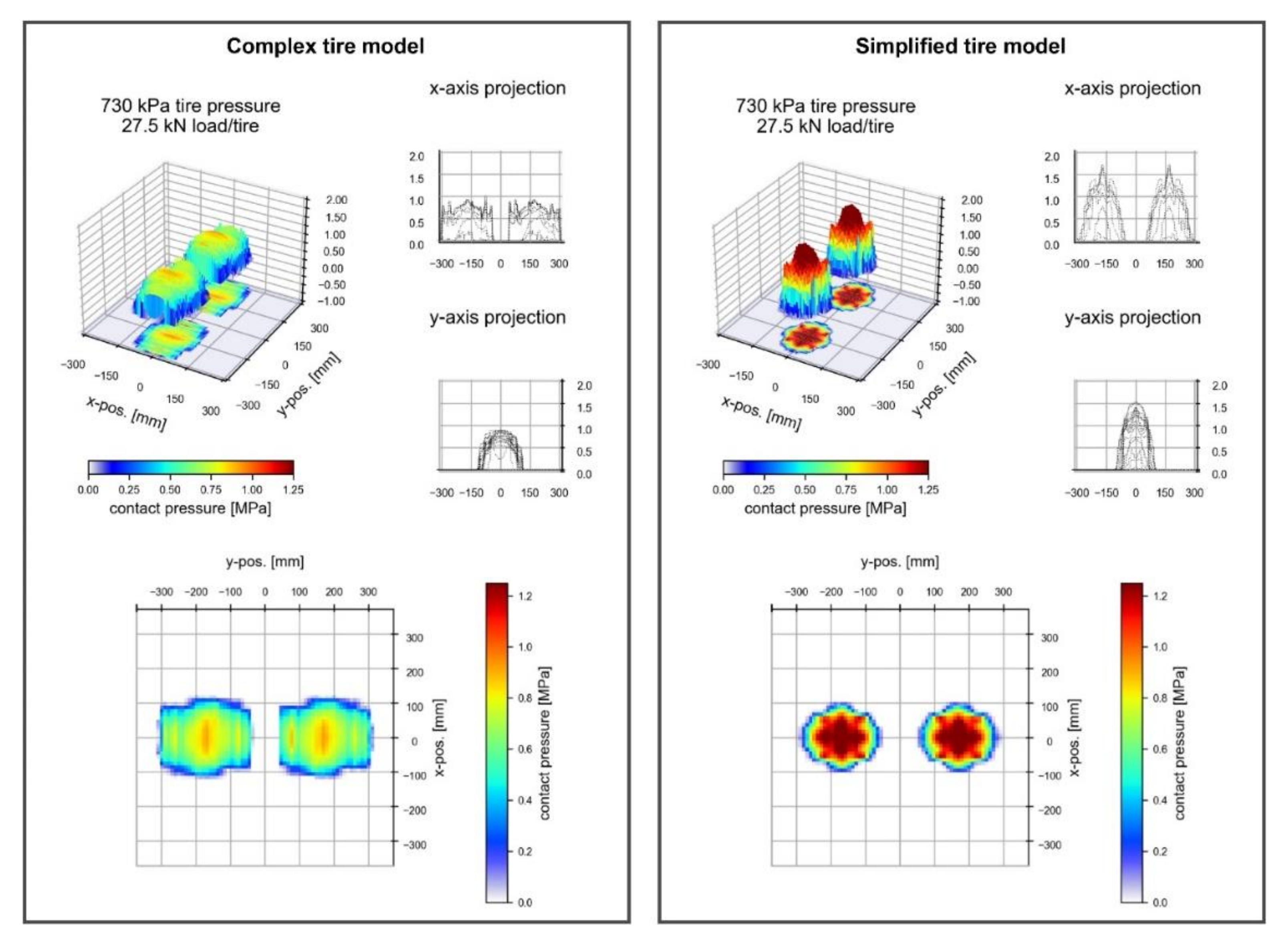
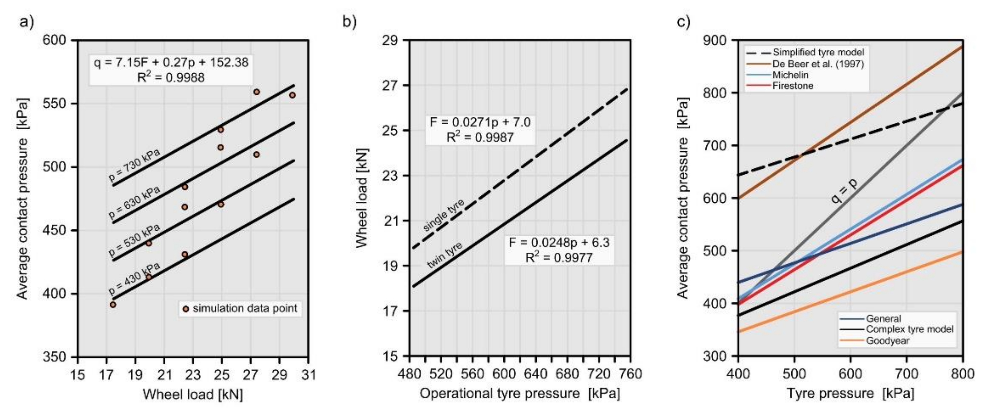
4.2. Comparison of the Behaviour of Finite Element Tyre Models

Differences between the two finite element tyre models were analysed at various tyre pressures and axle loads according to Table 6. The results consist of stresses in structures as well as contact areas and contact stresses of the tyre on the pavement, reflecting closely the results in the literature [25,26].
In the inflation process of the tyre models, it could be observed that the tight surface in the complex model first lay on and tightened to the rim of the body of wheel and, afterward, it tumbled over. The current, simple model was not able to describe this deformation process; consequently, the deformation of the sidewall was not the same during inflation. The treads of the two models show nearly the same deformation; however, looking at Figure 9, it can be observed that the tread rims of the simple model moved on a larger arc, which means that the middle of the tread received a higher part from the axle load.
Based on the finite element simulation, the contact area of the complex tyre model could be well approximated by a rectangle (see Figure 10). This answers to the behaviour of real radial tyres because these can be deformed only in the longitudinal direction and not in the transversal direction [27]. At the operational tyre inflation pressure and the highest allowed axle load, the distribution of contact stresses could be considered as an ellipsoid. However, in the case of low tyre pressure, the tread contacted the road surface unevenly; therefore, the middle of the tyre rose slightly, and the loading concentrated to the two sides of the tyre because of its stiffness. Consequently, the load distribution was not uniform and, according to Table 8, stress peaks ( q m a x ) may occur, reaching 2–3-fold of the average contact pressure. However, this did not cause a problem, if only the stresses in the wearing course or the rutting were analysed, because the surplus pressures were equalised at 5–8 cm below the road surface, according to the FEM model.
The simplified tyre model had a smaller contact area (that was because of smaller compression values; see Figure 10); moreover, it had a larger loading on the road pavement structure at the middle of the tread. The shape of the contact area was elliptical or circular, which is characteristic for diagonal tyres since it allows significant displacements in both directions to happen. Within the contact area of the simple tyre, three stress peaks could be observed, namely, in the middle, an elongated elliptical one and, next to it, on both sides, circular ones. The shape of the contact area confirmed the shape of the deformation, analysed during inflation.
The difference in the behaviour of the simplified tyre model can be explained mainly by the fact that the applied thin orthotropic plate-like shell element did not adequately describe the rebar of the tyre. The mechanical behaviour of the tyre is determined mainly by the construction of the carcass. Moreover, the layered shell elements react on shear stresses with a stiffer behaviour.
The next step of our research study was to establish a connection among the average contact pressure q, the wheel load F, and the inflation pressure of the tyre p. The empirical connection (5) of [11], based on laboratory tests, was applied (Figure 11a). The parameters of the function were determined by the least squares method using data from Table 6, as follows:
1.
In the case of the complex tyre model (R2 = 0.973),
q = 7.154 F + 0.272 p + 152.38 .  
2.
In the case of the simplified tyre model (R2 = 0.979),
q = 0.007 p F + 3.78 F + 545.56 .
In the case of the complex tyre model, the mixed effect of p and F could not be demonstrated, while, in the case of the simplified tyre model, the effect of the p inflation pressure vanished. The importance of the C prime constant, characterising the “flexibility” of the tyre, was also strengthened by the finite element simulation.
Considering the fact that tyre manufacturers provide values of allowable inflation pressure and wheel load for operation, Equations (7) and (8) can be further simplified (Figure 11b). The connection between the allowable wheel load and the inflation pressure of the tyre can be described by a linear function, according to the manufacturers’ data (R2 = 0.99):
F = 0.0248 p + 6.30 .  
Substituting Equation (9) into Equations (7) and (8), the connection between the average contact pressure under operational conditions and the inflation pressure can be described as follows:
1.
In case of the complex tyre model,
q = 0.449 p + 197.45 .
2.
In case of the simplified tyre model,
q = 0.000174 p 2 + 0.1378 p + 569.38 0.334 p + 512.57 .
Applying Equations (10) and (11), the average contact pressure q on the pavement surface can be estimated from the inflation pressure of the tyre p .
The author of [11], in his original paper, analysed the tyres of various manufacturers, i.e., Michelin, Firestone, Goodyear, and General, and, by averaging laboratory test results, obtained a linear connection (see Table 1) similar to that obtained in our research study. By plotting and comparing the two linear model equations (Figure 11c), it can be seen that the result of the complex finite element tyre model is close to the laboratory results of the Goodyear and General tyres, which proves our results. On the contrary, the results of the simplified tyre model significantly differ. However, in the work of [28], it was stated that the model of [11], in the case of plain surface diagonal tyres, underestimated the contact stress; therefore, in that case, its use is not recommended. Since, by the shape of the contact area, the behaviour of the simplified tyre model was more similar to diagonal tyres, it was worth comparing it with the modified model equation, as recommended by [28]:
q = 0.723 p + 310 .
In this case, the similarity is better; consequently, the behaviour of the simplified tyre model also describes a real tyre type. However, it is still true that the simplified finite element tyre model was not able to provide the behaviour of the complex tyre model since there were differences in the shape and size of the contact area as well as in the value and distribution of contact stresses. The variant behaviour of the two types of finite element tyre models was well described numerically by the C factor, which depends on the “flexibility” of the tyre.

4.3. Assessment of Tyre Models Considering the Road Pavement Structure

The stresses and strains in the flexible road pavement structure calculated by the two types of finite element tyre models, between two tyres of a twin tyre (at the axis of the twin tyre), are summarised in Table 9, while those straight below the tyre are summarised in Table 10. The first row of the tables’ heading contains the analysed points (from A to F) in the road pavement structure, illustrated in Figure 7. A significant difference is visible in case of the vertical u z z displacements or deflections below the tyre (Point D). This can be explained by the fact that the simplified tyre model had a higher contact stress at the direct contact point. The same explanation is valid for the higher ε y y specific strains in the lower part of the asphalt layer (Point E). These differences decreased at the axis of the twin tyre (Points A and B), since the contact area of the simplified tyre model was smaller; therefore, it had less effect on more distant places. The ε z z specific vertical compression values on the top of the subgrade (Points C and F) are in good correlation.
In practical calculations, i.e., pavement strengthening design, the loaded area of twin tyres is substituted by a circle of an area identical to the real contact area. The diameter of this substituting circle was also calculated in our research study, using the following equation:
a 564 F / q ,
where a is in mm and q is in kPa. The average contact pressure q is given by Equation (7) for the complex twin tyre model. The stresses and strains in the critical points of the flexible road pavement structure were calculated via WESLEA software, and they were compared to the results of the complex finite element twin tyre simulation (see Table 11 and Table 12).
The greatest differences occurred in the case of the vertical u z z displacements or deflections (Points A and D). The finite element pavement structure model—despite applying infinite elements—provided significantly lower (at 50–55%) values than the calculation based on the flexible-layer theory. This can be explained by the fact that WESLEA software, based on the theory of [13,14,15], summarises vertical specific displacements up to the infinite, providing supposedly higher displacement values than in reality. These high differences, observed in the case of deflections, require attention in the assessment of load-bearing capacity measurements based on vertical deflections, i.e., Benkelman beam, Lacroix, or Curviameter devices.
The values of the horizontal x- and y-direction ε x x and ε y y specific strains in the lower part of the asphalt layer (Points B and E) are in very good agreement with the results of the WESLEA software. In case of the vertical ε z z specific compression on the top of the subgrade (Points C and F), there was a slightly greater difference of 4–5%, the analytic solution being higher; however, it can still be regarded as being in good agreement. Based on the data in Table 11 and Table 12, it can be stated that stresses and strains for asphalt layer fatigue (Points B and E) and for subgrade compression (Points C and F) criteria can be accurately estimated by applying an evenly distributed load system on two circular plates substituting twin tyres, choosing the average contact stress q in a realistic way. In the case of the calculation of the critical deflection (Points A and D) for the vertical displacement criterium, this statement is not true. Further research is required for clarifying the cause of this phenomenon.

5. Summary

A complex finite element model of the tyre–pavement interaction was developed in this research study using ABAQUS finite element software. The developed model was sophisticated enough for the detailed analysis of the contact interaction; moreover, by applying appropriate material parameters, the model was also deemed suitable for further research work. In preparing the finite element simulation, considerable help was provided by the ABAQUS software manual [29], including many useful examples and pieces of information. Our results from the finite element simulation are in good agreement with literature data; therefore, a connection among the average contact pressure q , the wheel load F , and the inflation pressure of the tyre p was established. The results of our analysis show that the empirical equation published by [11], based on laboratory tests, can be appropriately applied for the determination of the average contact pressure q . Comparison calculations were performed using the average contact pressure q and the radius of the substituting circle of the tyre contact area on the pavement surface a in order to compare the performance of the finite element twin tyre simulation and the substituting circular plate model. The results of the finite element simulation are in good agreement with the results of WESLEA pavement structure design software, the only exception being the vertical u z z displacements or deflections. Critical stresses and strains for the asphalt layer fatigue and the subgrade compression criteria could be accurately determined by substituting the twin circular plate model.
Based on the complex rubber tyre model, a second, simplified tyre model was also developed in order to analyse the tyre–pavement interaction not only under static but also under dynamic conditions. The basic idea of keeping all material characteristics and only rebuilding the carcass applying composite shell elements did not prove to be a satisfactory direction. The results of the simplified model do not indicate the behaviour of the radial tyre, but rather of the diagonal tyre, regarding contact areas and stresses. It is possible that a better approximation of the layered structure of the complex radial tyre can be provided by using nominal material parameters, determined in an iterative way. Regarding the objective function, temporarily, the empirical model of [11] seems to be a good choice. Analysing stresses and strains in the flexible road pavement structure, the complex and the simplified models mainly provided similar results, concerning practical considerations. Therefore, the simplified model is also suitable for the design of a new or strengthened road pavement structure, as it has a considerably lower computational demand, which means that it is also suitable for analysing dynamic cases. The simplified tyre model makes it possible to further develop the finite element model of the road pavement structure, keeping its composition almost unaltered, incorporating viscoelastic or even viscoelastic–plastic material models and taking into account the displacement between layers.
Finally, the example of the two finite element tyre models, developed by different modelling approaches, indicates that the stiffness of rubber tyre models can vary in a wide range, even starting from the same geometry and materials. Consequently, our recommendation is that the simplified contact pressure model of any finite element tyre model is always published, as this would help the reproduction of research results by other researchers, even in the absence of originally used software.

Author Contributions

T.K., methodology, software, visualization, and review and editing; P.P. and C.T., conceptualization, methodology, formal analysis, and writing—original draft preparation. All authors have read and agreed to the published version of the manuscript.

Funding

This research study received no external funding.

Conflicts of Interest

The authors declare no conflict of interest.

References

  1. McCullough, B.F.; Boedecker, K.J. Use of Linear-Elastic Layered Theory for the Design of CRCP Overlays. Highw. Res. Rec. 1969, 2, 1–13. [Google Scholar]
  2. De Beer, M. Measurement of Tyre/Pavement Interface Stresses Under Moving Wheel Loads. Int. J. Heavy Veh. Syst. 1996, 3, 97–115. [Google Scholar] [CrossRef]
  3. Wang, H.; Hasan, O.; Al-Qadi, I.L.; Duarte, C.A. Analysis of Near-Surface Cracking under Critical Loading Conditions Using Uncracked and Cracked Pavement Models. J. Transp. Eng. 2013, 139, 992–1000. [Google Scholar] [CrossRef]
  4. Wang, G.; Reynaldo, R. Three-Dimensional Finite Element Modeling of Static Tire–Pavement Interaction. Transp. Res. Rec. J. Transp. Res. Board 2010, 2155, 158–169. [Google Scholar] [CrossRef]
  5. Hernandez, J.A.; Gamez, A.; Shakiba, M.; Al-Qadi, I.L. Numerical Prediction of Three-Dimensional Tire-Pavement Contact Stresses; Technical Report ICT-17-004; Taxas A&M University: College Station, TX, USA, 2017; Available online: http://hdl.handle.net/2142/95142 (accessed on 19 June 2020).
  6. Hernandez, J.A.; Al-Qadi, I.L. Semicoupled Modeling of Interaction between Deformable Tires and Pavements. J. Transp. Eng. Part A Syst. 2017, 143, 04016015. [Google Scholar] [CrossRef]
  7. Hernandez, J.A.; Angeli, G.; Maryam, S.; Imad, L. Al-Qadi. Tire–Pavement Interaction Modelling: Hyperelastic Tire and Elastic Pavement. Road Mater. Pavement Des. 2017, 18, 1067–1083. [Google Scholar] [CrossRef]
  8. Lawton, W.L. Static Load Contact Pressure Patterns under Airplane Tires. Highw. Res. Board Proc. 1957, 36, 233–239. [Google Scholar]
  9. Yoder, E.J. Principles of Pavement Design; John Wiley and Sons, Inc.: New York, NY, USA, 1959. [Google Scholar]
  10. Lister, N.W.; Nunn, D.E. Contact Areas of Commercial Vehicle Tyres; Transport and Road Research Laboratory: London, UK, 1968; Available online: https://trl.co.uk/sites/default/files/LR172.pdf (accessed on 23 April 2020).
  11. Van Vuuren, J.D. Relationship between Tire Inflation Pressure and Mean Tire Contact Pressure. Transp. Res. Rec. 1974, 523, 76–87. [Google Scholar]
  12. Kennedy, R.H. Experiences with Cylindrical Elements in Tire Modeling. In Proceedings of the ABAQUS Users’ Conference, Munich, Germany, 4–6 June 2003; Volume 247. Available online: http://www.simulia.com/download/solutions/automotive_cust%20references/tires_experience_auc03_hankook.pdf (accessed on 15 November 2019).
  13. Burmister, D.M. The General Theory of Stresses and Displacements in Layered Systems I. J. Appl. Phys. 1945, 16, 89–94. [Google Scholar] [CrossRef]
  14. Burmister, D.M. The General Theory of Stresses and Displacements in Layered Soil Systems II. J. Appl. Phys. 1945, 16, 126–127. [Google Scholar] [CrossRef]
  15. Burmister, D.M. The General Theory of Stresses and Displacements in Layered Soil Systems III. J. Appl. Phys. 1945, 16, 296–302. [Google Scholar] [CrossRef]
  16. Duncan, J.M.; Monismith, C.L.; Wilson, E.L. Finite Element Analyses of Pavements. Highw. Res. Rec. 1968, 228, 18–33. [Google Scholar]
  17. Yazdandoost, F.; Saied, T. Finite Element Tyre Model for Antilock Braking System Study. Int. J. Veh. Des. 2016, 72, 248–261. [Google Scholar] [CrossRef]
  18. Behroozinia, P.; Seyedmeysam, K.; Saied, T.; Reza, M. An Investigation towards Intelligent Tyres Using Finite Element Analysis. Int. J. Pavement Eng. 2020, 21, 311–321. [Google Scholar] [CrossRef]
  19. Van Blommestein, W.B. Experimentally Determined Material Parameters for Temperature Prediction of an Automobile Tire Using Finite Element Analysis. Ph.D. Thesis, Stellenbosch University, Stellenbosch, South Africa, 2016. [Google Scholar]
  20. Jeong, K.M. Prediction of Burst Pressure of a Radial Truck Tire Using Finite Element Analysis. World J. Eng. Technol. 2016, 4, 228–237. [Google Scholar] [CrossRef] [Green Version]
  21. Korunovic, N.; Miroslav, T.; Milos, S. FEA of tyres subjected to static loading. J. Serb. Soc. Comput. Mech. 2007, 1, 87–98. [Google Scholar]
  22. Wang, H. Analysis of Tire-Pavement Interaction and Pavement Responses Using a Decoupled Modeling Approach. Ph.D. Thesis, College of the University of Illinois, Urbana, IL, USA, 2010. [Google Scholar]
  23. Zhang, Z.; Hongxun, F.; Xuemeng, L.; Xiaoxia, C.; Di, T. Comparative Analysis of Static and Dynamic Performance of Nonpneumatic Tire with Flexible Spoke Structure. Stroj. Vestn. J. Mech. Eng. 2020, 66, 458–466. [Google Scholar] [CrossRef]
  24. Nakajima, Y. Advanced Tire Mechanics; Springer: Singapore, 2019. [Google Scholar] [CrossRef]
  25. Zhou, H.; Guolin, W.; Yangmin, D.; Jian, Y.; Chen, L.; Jing, F. Effect of Friction Model and Tire Maneuvering on Tire-Pavement Contact Stress. Adv. Mater. Sci. Eng. 2015, 2015, 1–11. [Google Scholar] [CrossRef] [Green Version]
  26. Wang, W.; Shan, Y.; Shugao, Z. Experimental Verification and Finite Element Modeling of Radial Truck Tire Under Static Loading. J. Reinf. Plast. Compos. 2013, 32, 490–498. [Google Scholar] [CrossRef]
  27. Gent, A.N.; Joseph, D.W. The Pneumatic Tire. DOT HS 810 561. The University of Akron. 2006. Available online: http://works.bepress.com/joseph_walter/7/ (accessed on 1 May 2019).
  28. De Beer, M.; Fisher, C.; Jooste, F.J. Determination of Pneumatic Tyre/Pavement Interface Contact Stresses Under Moving Loads and Some Effects on Pavements with Thin Asphalt Surfacing Layers. In Proceedings of the Eighth International Conference on Asphalt Pavements, Seattle, WA, USA, 10–14 August 1997; Larsen, H.J.E., Ed.; Road Directorate, Danish Road Institute: Roskilde, Denmark, 1997; Volume 1, pp. 179–227. [Google Scholar]
  29. Dassault Systèmes. Abaqus 6.14 Online Documentation. 23 April 2014. Available online: http://ivt-abaqusdoc.ivt.ntnu.no:2080/texis/search/?query=wetting&submit.x=0&submit.y=0&group=bk&CDB=v6.14 (accessed on 21 June 2020).
Figure 1. The power play of an absolutely flexible balloon (a) and a balloon with wall stiffness (b) contacting a smooth horizontal plane.
Applsci 12 02388 g001
Figure 2. The analysed domain of the road pavement structure and its finite element mesh.
Applsci 12 02388 g002
Figure 3. Cross-section view of radial tyre published by [5] (a); finite element mesh of the axial symmetric tyre model (b).
Applsci 12 02388 g003
Figure 4. Symmetric results for static 3D tyre analysis of the tyre–pavement interaction.
Applsci 12 02388 g004
Figure 5. Composite shell elements groups from 1 to 9 (transparent in the background, there is the complex tyre model).
Applsci 12 02388 g005
Figure 6. Example of a layered structure shell element: SH-120 element (#9) group with 9 layers.
Applsci 12 02388 g006
Figure 8. Comparison of the running time of simulation phases of complex and simple tyre models, where the top row shows the complex tyre model and the bottom row shows the simple tyre model.
Applsci 12 02388 g008
Figure 9. Comparison of deformation in the two types of finite element tyre models at 730 kPa pressure.
Applsci 12 02388 g009
Figure 10. Parts of interaction simulation results: the contact area and contact stress distribution of the complex FEM tyre model (left panel) and of the simplified FEM tyre model (right panel).
Applsci 12 02388 g010
Figure 11. The average contact pressure of the twin tyre depending on the inflation pressure and the (F/2) wheel load (a); the connection between the operational tyre pressure recommended by the manufacturer and the (F/2) wheel load (b); the connection between the average contact pressure and the operational tyre pressure (c).
Applsci 12 02388 g011
Table 1. Relationship among contact pressure, inflation pressure, and wheel load, according to [11].
Tyre TypesModel Parameters
a 1   a 2   b 1   C
07.50–15 Michelin Radial−0.002913.00.52052.0
08.25–20 × 10 Firestone Transport0.013010.50.119125.9
09.00–20 × 10 Firestone0.0240−0.9−0.001259.6
10.00–20 × 14 Papaleguas Goodyear Brazil0.00206.80.330110.0
11.00–20 × 14 General SDT0.00802.30.040313.0
11.00–22 × 14 General Jet Cargo0.00902.60.098211.0
Table 2. Layers and their linear elastic material characteristics in the analysed road pavement structure.
Layer NameThickness, h (mm)Young’s Modulus, E (MPa)Poisson’s Ratio, µ (-)
Asphalt wearing course4040000.35
Asphalt binder and base20055000.35
Crushed stone base2503500.40
Subgradeinfinite500.45
Table 3. Geometric dimensions of the composite structure of the DTA 275/80R22.5-type tyre.
#Tyre RegionMaterial NamePlyAngle (°)Cross-SectionDimension
(mm)
Spacing
(mm)
01treadtread rubberMAIN STRUCTURE
02sidewallsidewall rubber
03bead fillerbead rubber
04beadbead rubber
05rimcastor steel
06beltbelt steel150circleR 0.251.16
278circleR 0.251.16
3102circleR 0.251.16
478circleR 0.251.16
07carcasscarcass steel1+12circleR 0.400.80
2−12circleR 0.400.80
08chafer beltchafer belt steel190circleR 0.361.19
09nylon chaferchafer nylon190circleR 0.361.00
10steel chaferchafer steel190circleR 0.361.19
11strandswire steel8 × 690rectangle2.0 × 1.30.00
Table 4. Material parameters of the composite structure of the DTA 275/80R22.5-type tyre.
#Material NameModel of MaterialModel ParametersUnitLiterary Source
06belt steelElastic
(Hook)
ρ7.80 × 10⁻⁹t/mm3[18,19,22]
E174,700N/mm2
µ0.3-
11wire steelElastic
(Hook)
ρ5.90 × 10⁻⁹t/mm3[19]
E207,000N/mm2
µ0.3-
07carcass steelElastic
(Hook)
ρ1.39 × 10⁻⁹t/mm3
E16,870N/mm2
µ0.3-
08
10
chafer belt steelElastic
(Hook)
ρ1.50 × 10⁻⁹t/mm3
E9870N/mm2
µ0.3-
09chafer nylonElastic
(Hook)
ρ1.50 × 10⁻⁹t/mm3
E3970N/mm2
µ0.3-
01tread rubberHyper elastic
(Yeoh)
ρ1.10 × 10⁻⁹t/mm3[23]
C106.16 × 10−1N/mm2
C20−1.91 × 10⁻¹N/mm2
C304.75 × 10−2N/mm2
D18.12 × 10−2mm2/N
D28.12 × 10−2mm2/N
D38.12 × 10−2mm2/N
Viscoelastic
(Prony)
gi0.3-[18]
ki0.0-
τi0.1s
02sidewall rubberHyper elastic
(Yeoh)
ρ1.12 × 10⁻⁹t/mm3[17,23]
C104.88 × 10−1N/mm2
C20−1.41 × 10⁻¹N/mm2
C303.86 × 10−2N/mm2
D11.03 × 10−1mm2/N
D21.03 × 10−1mm2/N
D31.03 × 10−1mm2/N
Viscoelastic
(Prony)
gi0.3-[18]
ki0.0-
τi0.1s
03
04
bead rubberHyper elastic
(Yeoh)
ρ1.10 × 10⁻⁹t/mm3[18,23]
C108.76 × 10−1N/mm2
C20−2.93 × 10⁻¹N/mm2
C307.94 × 10−2N/mm2
D15.71 × 10−2mm2/N
D25.71 × 10−2mm2/N
D35.71 × 10−2mm2/N
Viscoelastic
(Prony)
gi0.3-[18]
ki0.0-
τi0.1s
05castor steelElastic
(Hook)
ρ7.80 × 10⁻⁸t/mm3[19]
E207,000N/mm2
µ0.3-
Table 5. Structural composition of the simplified tyre model.
#Shell Element DescriptionPlyThickness (mm)Material NameAngle (°)
1SH-340
tyre sidewall with strand
012.4002—sidewall rubber0
020.6107—carcass steel102
030.6107—carcass steel78
048.3803/04—bead rubber0
0510.011—wire steel0
068.3803/04—bead rubber0
070.6107—carcass steel102
080.6107—carcass steel78
092.4002—sidewall rubber0
2SH-280
tyre sidewall
015.0002—sidewall rubber0
020.4308/10—chafer belt steel0
035.0003/04—bead rubber0
040.4308/10—chafer belt steel0
050.6107—carcass steel102
060.6107—carcass steel78
0711.703/04—bead rubber0
080.6107—carcass steel102
090.6107—carcass steel78
103.0002—sidewall rubber0
3SH-200
tyre sidewall
015.0002—sidewall rubber0
020.4308/10—chafer belt steel0
038.6903/04—bead rubber0
040.6107—carcass steel102
050.6107—carcass steel78
064.6602—sidewall rubber0
4SH-140
tyre sidewall
018.5002—sidewall rubber0
020.6107—carcass steel102
030.6107—carcass steel78
044.2802—sidewall rubber0
5SH-120
tyre sidewall
015.9002—sidewall rubber0
020.6107—carcass steel102
030.6107—carcass steel78
044.8802—sidewall rubber0
6SH-170
tyre sidewall
0111.002—sidewall rubber0
020.6107—carcass steel102
030.6107—carcass steel78
044.7802—sidewall rubber0
7SH-170
tyre belt
013.0002—sidewall rubber0
020.2506—belt steel−12
030.2506—belt steel+12
040.2506—belt steel−12
054.8002—sidewall rubber0
060.6107—carcass steel102
070.6107—carcass steel78
087.2302—sidewall rubber0
8SH-140
tyre belt
012.0702—sidewall rubber0
020.2506—belt steel−12
030.2506—belt steel+12
040.2506—belt steel−12
053.9002—sidewall rubber0
060.6107—carcass steel102
070.6107—carcass steel78
086.0602—sidewall rubber0
9SH-120
tyre belt
010.9202—sidewall rubber0
020.2506—belt steel−40
030.2506—belt steel−12
040.2506—belt steel+12
050.2506—belt steel−12
062.8002—sidewall rubber0
070.6107—carcass steel102
080.6107—carcass steel78
096.0602—sidewall rubber0
Table 6. The tyre–pavement interaction simulation matrix.
Tyre Pressure (kPa)F/2 Load on One Tyre (kN)
Operation LoadOverloadExtreme Overload
43017.520.022.5
53020.022.525.0
63022.525.027.5
73025.027.530.0
Table 7. Element types and the number of elements applied in the two types of finite element tyre models.
Element TypeComplex Model (Per Tyre)Simple Model (Per Tyre)
Number of ElementsUsageNumber of ElementsUsage
Continuum element92,904all tyre parts and the body of wheel6000tread
Shell element0not applied2000body of wheel
Composite shell element0not applied4200all tyre parts except the tread
Membrane element10,500strengthening of the tyre,
carcass, belts etc.
0not applied
Total number of elements103,40412,200
Table 8. Results of the tyre–pavement interaction simulations.
F (kN)p (kPa)Complex Tyre FEM ModelSimple Tyre FEM Model
qmax (kPa)qavg (kPa)Proportion (-)qmax (kPa)qavg (kPa)Proportion (-)
17.54308013912.014647172.0
20.04309964142.414667002.1
22.543011924312.814756962.1
20.05307884411.815277302.1
22.55309324692.015497202.2
25.053011044712.315637292.1
22.56309324692.016087362.2
25.06309185161.816377472.2
27.563010315112.016517692.1
25.07309405311.816967592.2
27.57309715601.717227822.2
30.073010365571.917368162.1
Table 9. Stresses and strains in the flexible road pavement structure between two tyres of the twin tyre.
F/2
(kN)
p
(kPa)
ABC
uzzεxxεyyεzz
ComplexSimpleErrorComplexSimpleErrorComplexSimpleErrorComplexSimpleError
17.5430−0.190−0.1921.1%64,23166,6843.8%37,33834,519−7.5%−172,790−176,4052.1%
20.0430−0.217−0.2201.4%72,65176,1114.8%43,00639,733−7.6%−196,978−201,4652.3%
22.5430−0.244−0.2471.2%80,73785,4345.8%48,67845,019−7.5%−220,977−226,4802.5%
20.0530−0.217−0.2201.4%73,05576,1084.2%42,19539,607−6.1%−196,690−201,5112.5%
22.5530−0.243−0.2471.6%81,51185,4464.8%47,80844,861−6.2%−220,820−226,5342.6%
25.0530−0.270−0.2741.5%89,68494,6905.6%53,42450,143−6.1%−244,752−251,5112.8%
22.5630−0.242−0.2472.1%81,71885,4414.6%46,99844,708−4.9%−220,251−226,5692.9%
25.0630−0.269−0.2741.9%90,18094,7115.0%52,56349,978−4.9%−244,314−251,5773.0%
27.5630−0.296−0.3022.0%98,429103,9125.6%58,14255,279−4.9%−268,243−276,5103.1%
25.0730−0.268−0.2742.2%90,17894,7455.1%51,71449,824−3.7%−243,319−251,6303.4%
27.5730−0.294−0.3022.7%98,639103,9535.4%57,24055,073−3.8%−267,326−276,5843.5%
30.0730−0.321−0.3292.5%106,925113,1325.8%62,77660,406−3.8%−291,213−301,5043.5%
Table 10. Stresses and strains in the flexible road pavement structure straight below the tyre.
F/2
(kN)
p
(kPa)
DEF
uzzεxxεyyεzz
ComplexSimpleErrorComplexSimpleErrorComplexSimpleErrorComplexSimpleError
17.5430−0.194−0.2076.7%61,18765,1356.5%41,60746,35511.4%−161,948−165,2932.1%
20.0430−0.220−0.2356.8%69,01674,1977.5%46,94552,59512.0%−184,614−188,7672.2%
22.5430−0.246−0.2626.5%76,52083,1218.6%52,17458,76112.6%−207,093−212,1922.5%
20.0530−0.221−0.2356.3%69,71874,2556.5%47,70052,75710.6%−184,361−188,8142.4%
22.5530−0.247−0.2636.5%77,59483,2007.2%53,07158,95211.1%−206,668−212,2492.7%
25.0530−0.273−0.2916.6%85,19692,0298.0%58,33465,09511.6%−229,390−235,6382.7%
22.5630−0.248−0.2636.0%78,08583,2676.6%53,68959,12010.1%−206,455−212,2922.8%
25.0630−0.274−0.2916.2%85,97992,1327.2%59,08165,30910.5%−228,999−235,7092.9%
27.5630−0.299−0.3196.7%93,665100,9057.7%64,38971,39310.9%−251,421−259,0623.0%
25.0730−0.274−0.2926.6%86,24992,2116.9%59,53865,48810.0%−228,086−235,7653.4%
27.5730−0.300−0.3196.3%94,152101,0127.3%64,94871,63710.3%−250,578−259,1383.4%
30.0730−0.326−0.3476.4%101,884109,7507.7%70,28677,69010.5%−272,961−282,4813.5%
Table 11. Critical stresses and strains between two tyres based on the twin tyre finite element simulation (FEM) and the substituting circular plate model (MLEA).
F/2
(kN)
q
(kPa)
ABC
uzzεxxεyyεzz
FEMMLEAErrorFEMMLEAErrorFEMMLEAErrorFEMMLEAError
17.5385−0.190−0.29354.5%64,23162,750−2.3%37,33835,800−4.1%−172,790−179,1503.7%
20.0408−0.217−0.33554.5%72,65171,230−2.0%43,00641,280−4.0%−196,978−204,3903.8%
22.5430−0.244−0.37754.6%80,73779,570−1.4%48,67846,840−3.8%−220,977−229,5403.9%
20.0415−0.217−0.33554.5%73,05571,620−2.0%42,19540,990−2.9%−196,690−204,6704.1%
22.5438−0.243−0.37755.2%81,51180,200−1.6%47,80846,390−3.0%−220,820−229,9904.2%
25.0460−0.270−0.41955.2%89,68488,270−1.6%53,42452,140−2.4%−244,752−254,9504.2%
22.5445−0.242−0.37755.9%81,71880,420−1.6%46,99846,230−1.6%−220,251−230,1504.5%
25.0468−0.269−0.41955.8%90,18089,030−1.3%52,56351,610−1.8%−244,314−255,4904.6%
27.5491−0.296−0.46155.7%98,42996,950−1.5%58,14257,460−1.2%−268,243−280,3304.5%
25.0475−0.268−0.41956.4%90,17889,250−1.0%51,71451,450−0.5%−243,319−255,6405.1%
27.5498−0.294−0.46156.8%98,63997,820−0.8%57,24056,850−0.7%−267,326−280,9505.1%
30.0521−0.321−0.50356.7%106,925105,780−1.1%62,77662,680−0.2%−291,213−305,8305.0%
Table 12. Critical stresses and strains straight below the tyre based on the twin tyre finite element simulation (FEM) and the substituting circular plate model (MLEA).
F/2
(kN)
q
(kPa)
DEF
uzzεxxεyyεzz
FEMMLEAErrorFEMMLEAErrorFEMMLEAErrorFEMMLEAError
17.5395−0.194−0.29552.1%61,18760,080−1.8%41,60742,7302.7%−161,948−168,5404.1%
20.0412−0.220−0.33652.7%69,01667,970−1.5%46,94548,2702.8%−184,614−192,2804.2%
22.5430−0.246−0.37853.7%76,52075,690−1.1%52,17453,6702.9%−207,093−215,9204.3%
20.0440−0.221−0.33752.5%69,71868,530−1.7%47,70048,7202.1%−184,361−192,5504.4%
22.5458−0.247−0.37953.4%77,59476,560−1.3%53,07154,3802.5%−206,668−216,3604.7%
25.0475−0.273−0.41953.5%85,19683,910−1.5%58,33459,4802.0%−229,390−239,8104.5%
22.5485−0.248−0.37952.8%78,08576,870−1.6%53,68954,6301.8%−206,455−216,5104.9%
25.0503−0.274−0.42153.6%85,97984,960−1.2%59,08160,3302.1%−228,999−240,3405.0%
27.5520−0.299−0.46154.2%93,66592,100−1.7%64,38965,2601.4%−251,421−263,6904.9%
25.0530−0.274−0.42153.6%86,24985,250−1.2%59,53860,5701.7%−228,086−240,4905.4%
27.5548−0.300−0.46254.0%94,15293,290−0.9%64,94866,2302.0%−250,578−264,2905.5%
30.0566−0.326−0.50354.3%101,884100,490−1.4%70,28671,2101.3%−272,961−287,6705.4%
Publisher’s Note: MDPI stays neutral with regard to jurisdictional claims in published maps and institutional affiliations.

