Abstract
Methane is the second most important greenhouse gas after carbon dioxide. The intensity and distribution of methane source/sink in China are unknown. We collected the column-averaged dry air mixing ratio of CH4 (abbreviated as XCH4 hereafter) from TROPOMI for the period from 2018 to 2021, to study spatial distribution and temporal change of atmospheric CH4 concentration, providing clues and foundations for understanding the source/sink in China. It was found that the distribution of XCH4 is roughly high in the East, low in the West, high in the South and low in the North. Additionally, an evidently positive linear relationship between XCH4 and population density was witnessed, suggesting anthropogenic emissions may account for a large portion of total methane emissions. XCH4 exhibits evident seasonal characteristics, with the peak in summer and trough in winter, regardless of the different regions. Moreover, we used XCH4 anomalies to identify the emission sources and found its great potential in the detection of methane emission from mining plants, landfill, rice fields and even geological fracture zones.
1. Introduction
China set its carbon neutrality target in 2020, claiming to peak its carbon emissions by 2030 and achieve net zero carbon emissions by 2060 [1]. Methane is the second most important greenhouse gas after carbon dioxide directly influenced by anthropogenic activity, and its radiative forcing is close to that of all other non-CO2 greenhouse gases combined in time and space [2]. Methane has more than 80 times the warming power of carbon dioxide over the first 20 years after it reaches the atmosphere [3]. Even though CO2 has a longer-lasting effect, methane currently sets the pace for warming [4]. Recent studies confirmed that the atmospheric concentration of CH4 reached an unprecedented level since records began, exhibiting an accelerating upward trend [5]. However, unlike CO2 emissions, methane emissions have not been well understood in both developed and developing countries [6,7,8]. For example, China, to date, has not yet compiled its own CH4 emission inventory. Hence, there is a large gap between China’s carbon neutrality ambition and the reality, considering methane emissions. Consequently, understanding the temporal and spatial distribution of the atmospheric concentration of CH4 in China is of great significance, and is an urgently critical step for subsequent compilation of CH4 emission inventory.
For an insight into the spatial and temporal distributions of atmospheric CH4 concentrations, several studies have been conducted using observations obtained by different platforms and techniques. Previously, researchers used XCH4 provided by SCIAMACHY and AIRS to study the spatial–temporal variations of CH4 over China and infer methane emissions [9,10,11,12,13,14]. Wu monitored the temporal and spatial variation characteristics of atmospheric CH4 concentrations in China, from 2002 to 2016, using atmospheric infrared detector (AIRS), and found hot spots of XCH4 in Northern Xinjiang, Northeast Heilongjiang and Northwest Sichuan [15]. Since the launch of the GOSAT satellite, XCH4 dataset provided by GOSAT soon became a widely used product to monitor atmospheric CH4 concentrations at a large spatial scale due to its better performance. Since then, satellite-derived XCO2 products have been validated with XCO2 observations obtained by ground-based networks consisting of Fourier transform spectrometers (FTSs), demonstrating reliable performances [16,17,18,19]. Compared with the above sensor data, TROPOMI (the tropospheric monitoring instrument) has its unique advantages, providing XCH4 products with a much higher spatial resolution, a better coverage as well as rapid revisits. Previous studies have shown that XCH4 products of TROPOMI exhibit an adequate reliability and accuracy [20,21,22]. Therefore, many research teams used TROPOMI data for CH4 observation [23,24,25,26]. However, XCH4 of TROPOMI is more affected by surface albedo and has larger biases compared to GOSAT [27].
XCH4 products from TROPOMI provide a new and valuable opportunity to gain insight into the temporal and spatial variations of CH4 in China. Moreover, its wider coverage and finer spatial resolution enable us to further explore the feasibility of identifying CH4 emission hotspots on a small scale, such as oil fields [28] and mineral exploration.
In the present study, we collected XCH4 products from TROPOMI for the period from 2018 to 2021, analyzed the temporal and spatial distribution patterns of the atmospheric CH4 concentrations in China and tried to identify the plausible reasons behind such distribution patterns. Different spatial analysis techniques, such as correlation analysis, spatial autocorrelation, high-low cluster and cold-hot spot analysis, were utilized to achieve our goals.
The remaining parts of this work are organized as follows. Section 2 introduces data sources and processing methods. Section 3 demonstrates the spatial and temporal distribution of atmospheric CH4 concentrations in China over land. Additionally, we also present the CH4 anomalies in some typical places in this section. We discuss the outcomes and plausible reasons in Section 4. Finally, we summarize the whole work in Section 5.
2. Materials and Methods
2.1. Data Source
The XCH4 product used in this study was provided by TROPOMI, a multispectral sensor carried on the Sentinel-5p, of which the spatial resolution is 0.01 radians and the revisit period is 17 days. In this study, the monthly XCH4 products in China, spanning from May 2018 to May 2021, were acquired from GES DISC (NASA Goddard earth sciences data and the Information Services Center, https://disc.gsfc.nasa.gov/, accessed on 10 November 2021). The seasonal and yearly XCH4 products, spanning from March 2020 to March 2021, were acquired via the GEE (Google Earth engine) platform. The earliest date for the XCH4 product provided by the GEE platform is March 2019, and that for GES DISC is May 2018. Therefore, the latter was chosen for the temporal variation analysis to provide a sufficiently long time span. Herein, the spring period is defined as March, April and May; the summer period is defined as June, July and August; the autumn period is defined as September, October and November and the winter period is defined as December, January and February. The XCH4 product provided by the GEE is the level-3 product. The minimum value is 1491 ppbv (parts per billion) and the maximum value is 2352 ppbv. The angle resolution is 0.01 radian and the spatial resolutions at the nadir points are 3.5 × 7 km2 and 7 × 7 km2 in the study period. For convenience, the spatial resolutions were resamples to 10 × 10 km2 on the GEE platform. The value of each pixel in the final output data is the average of all the pixels in the given grid with a certain time period. The data retrieved from GEE was filtered with the condition that the QA value (data reliability) was better than 0.5.
In this work, we selected four study areas (as Figure 1 shows): TARIM Basin (78° E–88° E, 37° N–42° N), Sichuan Basin (103° E–108° E, 28° N–32° N), Central China (110° E–118° E, 26° N–32° N) and North China (114° E–119° E, 32° N–37° N). The time period is from May 2018 to May 2021.
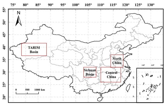
Figure 1.
Location of the four study areas.
2.2. Data Processing Method
2.2.1. Correlation Analysis
The correlation analysis is used to measure the correlation between the two variables. This paper uses the correlation coefficient to reflect the correlation between population density and CH4 concentration. The value of the correlation coefficient is between 1 and −1. The number 1 means that the two variables are completely linear in correlation, while −1 means that the two variables are completely negative in correlation. Additionally, zero means that the two variables are not correlated. The more the data tends to zero, the weaker the correlation.
2.2.2. Spatial Autocorrelation Analysis
Spatial autocorrelation refers to the potential interdependence of some variables in the same distribution area between the observed data [29]. Moran’s I, Z-score and p-value were recognized as the indices to evaluate the significance.
The value of Moran index I is between −1 and 1; less than zero indicates a negative correlation; equal to zero indicates statistically uncorrelated and greater than zero indicates a positive correlation [30]. Moran’s I index is calculated as follows:
where is the deviation of element i’s attribute and its average value , is the spatial weight between elements and , is the total counts of elements and is the aggregation of all spatial weights:
The p-value represents the probability that the observed spatial pattern is created by a random process. When the p-value is very small, it means that the observed spatial pattern is unlikely to arise from random processes. The Z-score represents the multiple of the standard deviation. The larger the value of the Z-score is, the higher the confidence that it is unlikely to occur from the random process.
2.2.3. High–Low Cluster Analysis and Cold–Hot Spot Analysis
The high–low cluster analysis can measure the clustering degree of high or low values, which is actually used to measure the density of high values or low values in the study area.
The cold–hot spot analysis is used to identify the significant spatial clustering of high values (hot spot) and low values (cold spot). This tool creates a new output feature class for each feature in the input feature class using the Z-scores, p-value and confidence intervals. If the Z-score of the feature was high and the p-value was small, it would indicate that there is a high-value spatial clustering. On the contrary, if the Z-score is low and negative and the p-value is small, it indicates that there is a spatial cluster with a low value. The higher (or lower) the Z-score, the greater the degree of clustering. If the Z-score is close to zero, it indicates that there is no obvious spatial clustering.
2.2.4. Time Series Data Processing Method
When studying the temporal trend of CH4 emissions in China, four regions with large CH4 emissions (TARIM Basin, Sichuan Basin, Central China and North China) were selected, so as to ensure there were adequate datasets to participate in the monthly mean value calculation. Therefore, we can eliminate the occurrence of accidents and ensure the reliability of the results. In processing the monthly average data of the study area, firstly, reading the data within the longitude and latitude of the study area and QA-value is greater than 0.75. Then, eliminate the data with large distances from the mean value (the absolute value of subtracting the mean is greater than 30) in the data of this month, to ensure the data variance within one month is reasonable, because the CH4 concentration will not change much within one month. Finally, the monthly average value of XCH4 was calculated using the remaining data.
3. Results
3.1. Spatial Distribution of XCH4
Figure 2 shows the distribution of the average XCH4 within China for two years from 2019 to 2021. Figure 2 shows that the overall XCH4 in China is high in the East, low in the West, high in the North and low in the South. In particular, XCH4 is lower in the Inner Mongolia Autonomous Region and Northeast China, above 45° N latitude, than in other places. North China, Central China, South China, the Sichuan Basin and TARIM Basin are areas with relatively high XCH4, while the Northeast and Qinghai–Tibet Plateau witnessed relatively low XCH4. XCH4 takes values in the range of 1753 to 1978 ppm. Figure 3 shows the population distribution in China. The spatial distribution of the population exhibits a similar pattern with the XCH4. The vast majority of the population is distributed in the east of the Heihe–Tengchong Line, of which North China is the most densely populated place. The place with the highest CH4 concentration in China, shown in Figure 2, is also North China. In addition, Central China and the Sichuan Basin are also places with a high CH4 accumulation and high population density. To quantify this apparently existing correlation, we performed a correlation analysis between the population density and the XCH4 concentration at the provincial scale. Such an analysis was performed by selecting all the provinces in the east of the Heihe–Tengchong Line to eliminate the sampling bias due to insufficient observations in the western provinces. We took each province as the unit of calculation. The horizontal coordinate is the mean population density and the vertical coordinate is the XCH4 annual mean. It yielded a high correlation with R of 0.84, as shown in Figure 4, for which it can be considered that the CH4 concentration and population density are positively correlated. The determination coefficient of the XCH4 population relationship is 0.7, suggesting the population distribution can largely explain the spatial distribution characteristics of XCH4. A previous study indicated that 85% of methane emissions are related to human activities in China [31]. Given that there is a positive relationship between XCH4 and methane emissions, satellite-derived XCH4 products also suggest that anthropogenic emissions are probably the main source of the methane emissions in China. The population density could be a good proxy to map a gridded methane inventory with a high resolution in the future.
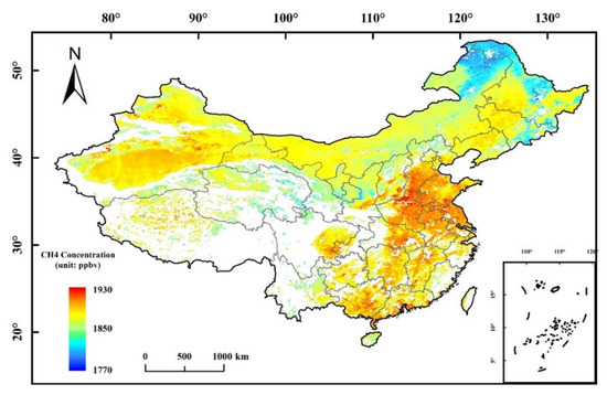
Figure 2.
Annual average distribution of CH4 in China from 2019 to 2021.
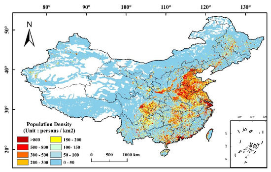
Figure 3.
Distribution map of population density in China in 2020.
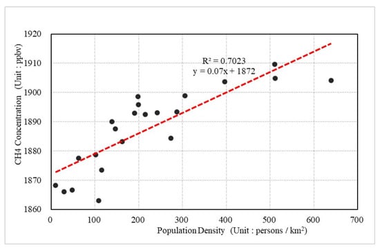
Figure 4.
Scatter plot of population density and CH4 concentration.
The variation of XCH4 exhibits an evident seasonal characteristic. Figure 5 shows the distribution of XCH4 in China in four seasons. We can find that the XCH4 distribution in different seasons is similar with its annual distribution. Overall, the CH4 concentration is higher in summer and autumn than that in spring and winter. Different regions exhibit different seasonal characteristic. For example, in North China, the XCH4 is typically high in summer and autumn, low in spring and winter and the concentration changes significantly. In Northern Heilongjiang, XCH4 is low in all seasons, and there is no large gap in the CH4 concentration in all seasons. However, it can also be observed that the XCH4 in this place is high in summer and winter, and low in spring and autumn, with the highest levels in winter and the lowest in spring, which is different from the other places. In the Qinghai–Tibet Plateau, due to the high terrain, complex terrain and lack of observation data, the variation of XCH4 in the four seasons cannot be observed in the Figure.
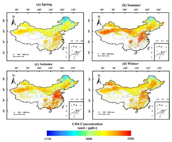
Figure 5.
Distribution of CH4 in China from 2019 to 2021. (a) Spring, (b) summer, (c) Autumn, (d) Winter.
We utilized the spatial autocorrelation analysis, high–low cluster analysis and cold–hot spot analysis to gain an insight into understanding the spatial distribution characteristics of XCH4. The spatial autocorrelation analysis yielded a Moran index I of 0.78 and a Z-score of 2060, with a p-value less than 0.01, indicating a positive spatial correlation of XCH4 with high confidence. It is thus considered that there should be clustering in the spatial distribution of XCH4. Additionally, the geographically adjacent regions tend to have the same properties in terms of XCH4 distribution.
Figure 6 shows the results obtained by the cluster analysis. Figure 6 demonstrates that there are high–high clusters in the middle and east of China, the TARIM Basin and JUNGGAR Basin, and low–low clusters in the east of Inner Mongolia, north of Heilongjiang, east of the three northeastern provinces and east of Gansu and Hainan. There is no significant clustering in the west of Inner Mongolia and the area where Inner Mongolia and the three northeastern provinces connect. There are few high–low clusters and low–high clusters, which exist in sporadic areas at the junction of the high value and low value. In Western Sichuan and the Qinghai–Tibet Plateau, cluster analysis cannot be carried out due to the lack of data.
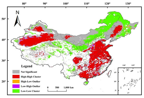
Figure 6.
Cluster analysis of CH4 concentration.
In addition, the analysis of the cold and hot spots was also carried out to measure the density of the high values or low values in China in Figure 7. The spatial distribution of CH4 in China is more scientifically verified by the cold and hot spot analysis map. With 99% confidence, we believe that the central and eastern parts of China, the central parts of the three northeastern provinces, the TARIM Basin, the JUNGGAR Basin, the Sichuan Basin and the EJINA Banner in western Inner Mongolia are the hot spots of CH4 emissions. With 99% confidence, we also believe that the central and eastern parts of Inner Mongolia, the eastern parts of the three northeastern provinces and Hainan Island are the cold spots of CH4 emissions. Only in a few places is there no significant indication of cold spots or hot spots.
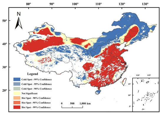
Figure 7.
Analysis results of cold and hot spots in China.
3.2. Temporal Variation of CH4 in China
As XCH4 products are inadequate in several places every month from May 2018 to May 2021 in China, we selected 4 representative areas to study the temporal variation characteristics of CH4 concentrations in China. The selection criterion is that the area has sufficient data (data availability ratio is better than 50%) to calculate the monthly average concentration every month. Four areas were selected: North China, Central China, the Sichuan Basin and the TARIM Basin. Figure 8 shows the temporal trend of the mean XCH4 in the above four regions.
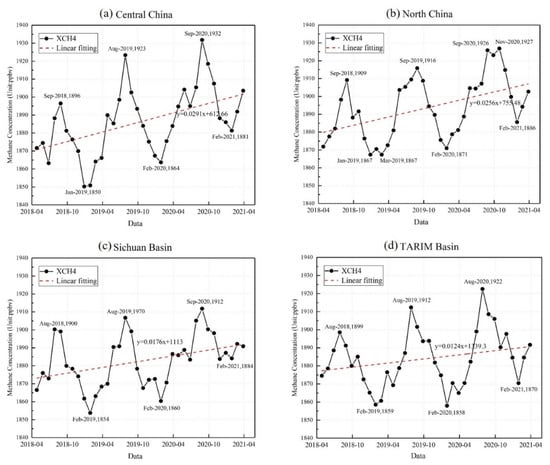
Figure 8.
Temporal variation of CH4 in the study area, (a) Central China, (b) North China, (c) Sichuan Basin, (d) TARIM basin.
Figure 8a–d illustrate that there are evident periodical characteristics with a period of one year in all four regions. XCH4 is rising at different growth rates in four regions. The greatest annual growth of XCH4 was witnessed in Central China, while the smallest was witnessed in the TARIM Basin. From the perspective of seasonal variation, XCH4 reaches its peak in August or September and then falls to its valley in January or February. The differences between the maximum and minimum XCH4 levels within one year, vary from 58 ppb (in the Sichuan Basin) to 82 ppb (in Central China), implying that the intensity of terrestrial ecosystem methane emissions varies significantly across regions.
We can then conclude from the above results that both the annual growth and the amplitude of XCH4 vary in terms of different regions, which suggest that there is an evident spatial heterogeneity in the methane emissions regardless of natural and anthropogenic emissions.
3.3. Anomaly of CH4 and Its Significance
Compared with the XCH4 itself, its anomaly can better highlight potential methane emissions because the background concentrations that are determined by regional scale emissions and transportations are subtracted. The XCH4 anomaly was defined and extracted from the original products based on Equation (3):
where is the original XCH4 retrieval, is the median of in the given region (methane emission anomaly Study area) in a month and is the resultant anomaly.
After extracting the XCH4 anomalies, we further used such products to explore hotspots that were likely related with methane emissions. In this section, we focus on four representative methane-emitting regions to explore the ability of the XCH4 anomaly to identify methane emissions.
3.3.1. Mining Operations
Shanxi Province is a major energy province of China, mainly for coal mining. Figure 9 demonstrates the spatial distribution of XCH4 anomalies in Shanxi. We can see that XCH4 anomalies exceed 40 ppb in parts of Shanxi, such as in Yangquan, Changzhi and Jincheng. All these regions are famous for their coal mines. The results indicate that XCH4 anomalies derived from TROPOMI products can be used to map XCH4 enhancements due to methane emissions related to coal mining at a city scale. Furthermore, we tried to identify strong point sources of methane due to the mining industry using XCH4 anomalies.
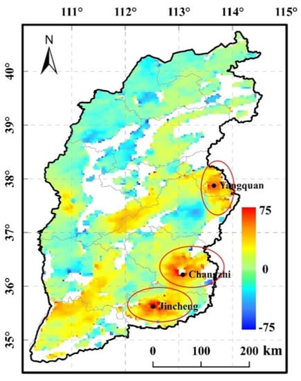
Figure 9.
High CH4 concentrations in Yangquan, Changzhi and Jincheng.
Figure 10 shows a typical positive XCH4 anomaly in the southern Ejina Banner (100.0° E, 41.1° N) of Alxa League, the Inner Mongolia Autonomous Region, the junction of Inner Mongolia and Gansu. The visual interpretation of a high resolution image indicates that the plant is located in the middle of the Gobi desert where other methane emissions are rare. Figure 10 shows that there is an XCH4 anomaly of about 40 ppb in the surroundings of an open pit coal mine. We can thus conclude that the aXCH4 products of TROPOMI have great potential to identify strong point source methane emissions when not influenced by other methane fluxes.
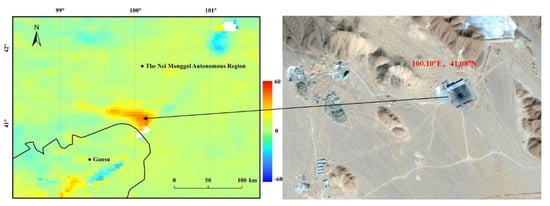
Figure 10.
A stable high value anomaly of CH4 at the border of Inner Mongolia and Gansu.
3.3.2. Landfill
Figure 11 shows a high value anomaly of CH4 in the north of Jinan (117.01° E, 36.86° N). Through high-resolution satellite images, we found a large-scale landfill site in the northwestern part of the built-up area of the city. Furthermore, a higher anomaly with a larger area at the northwestern region coincides with a number of oil and gas storage tanks.
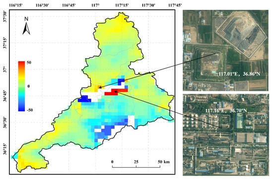
Figure 11.
A high value anomaly of CH4 in Jinan.
3.3.3. Rice Producing Area
Figure 12 shows a close-up of the CH4 distribution in Wuhan and Xiaogan. It can be clearly seen that there is a large area of high CH4 value at the junction at the west of the Caidian District in Wuhan and the south of Hanchuan City in Xiaogan. The high value area is connected to a large area, which is 20–40 ppb higher than the background. The Jianghan Plain was a large lake 2000–3000 years ago, and then gradually evolved into a plain area. Compared to the plains of North and Northeast China, large wetlands still exist in the Jianghan Plain today [32]. These wetlands have been artificially modified to form large areas of rice fields. Fish and shrimp are also extensively farmed in these rice fields and have become an important source of local economy. According to the report from the European Commission, wetlands and rice account for more than 30% of the total global methane emissions [33]. Gong et al. found that paddy fields accounted for 19% of the total emissions [31]. Through high-resolution satellite images, it can be seen that there are a large areas of paddy fields in this area. Meanwhile, there are no other known sources of methane emissions in the area, as illustrated in Figure 12. Therefore, such anomalies could be direct evidence for paddy fields. Similar XCH4 anomalies caused by paddy fields are also seen in other major rice producing areas, such as Hunan, Anhui and Northeast China.
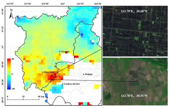
Figure 12.
A large area of CH4 high value anomaly in Western Wuhan.
3.3.4. Geological Structure
Figure 13 shows that there is an evident CH4 anomaly in the west (79.8° E, 41° N) of the Aksu region. The region is inaccessible and there are hardly any signs of anthropogenic activity. High-resolution satellite images show a very distinctive large fold phenomenon. At the same time, the black rock layers suggest that the area is likely to be rich in coal and natural gas. Hence, such an XCH4 anomaly is likely related with CH4 leakage due to the fault zone.
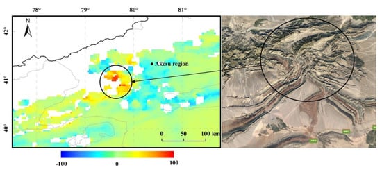
Figure 13.
High value anomaly of CH4 in the Aksu area, Xinjiang.
4. Discussion
Anthropogenic methane emissions may account for a high proportion of total methane emissions in China. It is can be observed that the spatial distribution of XCH4 is basically consistent with the population distribution in China. In Eastern China, there is a dense population and more human activity. That area exhibits a high level of XCH4. The Qinghai–Tibet Plateau, northern Inner Mongolia and northern Heilongjiang are sparsely populated and have fewer human activities. Those regions correspondently exhibit a low level of XCH4. Xinjiang may be an exception. Despite its low population density, its well-developed oil and gas industry has led to relatively high levels of XCH4 in the region.
In Northern China, there is a large population and frequent human activity, especially in Beijing, Tianjin, Hebei and Shandong, which have a large population density, developed industry and consume a large amount of fossil fuels, resulting in a large amount of CH4 accumulation. Several northern provinces are also major livestock provinces. The development of livestock will also lead to an increase in CH4 emissions. The high CH4 emission area in Northeast China may be related to oil field exploitation and a large area of wetlands. Anthropogenic methane emissions, such as energy activities, livestock, wastewater and municipal solid waste contribute over 65% of the total emissions in China, according to a recent study [31]. This explains why XCH4 is positively related with the population.
Figure 8 shows that the XCH4 in China reaches its peak in September every year. Such a phenomenon is consistent with SCIAMACHY’s observations in China [34]. Chandra, N et al. indicated that agricultural practices, i.e., paddy fields as well as large scale transport and chemistry, are responsible for the high methane concentration during that season. The low XCH4 in winter, namely in December, January and February, is mainly due to the seasonality of emissions from wetlands, vegetation and rice paddies.
In Central and Southern China, the high XCH4 level is related to the rice paddies and vegetation. The rice planted in these areas is two or three crops a year, which will emit a large amount of CH4 into the atmosphere during the rice growth season. The monthly average XCH4 in Central China changes dramatically within a year, which could be related to the existence of large areas of paddy fields in this region. In August and September, rice ripens and releases a large amount of CH4, resulting in the peak of XCH4 in Central China at this time. After the rice harvest, XCH4 decreases rapidly until January in winter. Arriving in spring in March, agricultural activities begin to recover and gradually increase, and then CH4 concentrations began to rise correspondingly. Similar patterns were used for emissions caused by other vegetation.
Although the TARIM Basin is sparsely populated, there are a lot of energy activities. The TARIM Basin contains quite rich oil and natural gases. It is an important energy production base in China and the starting point of the “West–East Gas Transmission” project. The exploitation of oil and natural gas would leak a large amount of CH4. Therefore, XCH4 in the TARIM Basin are maintained at a high level throughout the year.
The Chengdu Plain, known as the “land of abundance” in the Sichuan Basin, has a large population. There are many anthropogenic emissions, such as livestock breeding, energy activities and rice planting, which all contribute to the high XCH4 here. Among them, energy activities lead to the maintenance of CH4 concentrations in this area at a high level. Rice planting and livestock breeding are the main causes for seasonal fluctuations in XCH4 within a year.
5. Conclusions
This paper presented a quantitative study on the temporal and spatial distribution of CH4 concentrations in China. Our results found that the distribution of XCH4 is roughly high in the East, low in the West, high in the South and low in the North. Through visual interpretation and correlation analysis with population data, we concluded that the spatial distribution of XCH4 in China has a great correlation with the population distribution. In addition, XCH4 is generally high in summer and low in winter. Furthermore, four regions with adequate XCH4 observations were selected for time series analysis. We found that XCH4 generally exhibits a certain temporal periodicity. The cycle is one year, reaching the peak in summer and the trough in winter. However, some monthly average XCH4 observations are abnormal, and the reasons need to be further explored. This paper also demonstrated the XCH4 anomaly in China. Evident XCH4 anomalies were witnessed at coal mining plants, landfills, rice field production areas and coal-bearing geological fracture zones. In the future, it is a very meaningful task to quantitatively estimate the intensities of methane sources using XCH4 anomalies.
Author Contributions
Conceptualization, W.G.; investigation, H.M.; methodology, X.M.; writing—original draft, J.Z. and Z.P.; writing—review and editing, G.H.; revision and review, W.J. All authors have read and agreed to the published version of the manuscript.
Funding
This work was supported by the National Natural Science Foundation of China (Grant No. 41971283, 41901274, 41971352) and the Major Project of High Resolution Earth Observation System (Grant No. GFZX0404130302).
Conflicts of Interest
The authors declare no conflict of interest.
References
- Cao, Y.; Li, X.M.; Yan, H.B.; Kuang, S.Y. China’s efforts to peak carbon emissions: Targets and practice. Chin. J. Urban Environ. Stud. 2021, 9, 2150004. [Google Scholar] [CrossRef]
- Supharatid, S. Assessment of cmip3-cmip5 climate models precipitation projection and implication of flood vulnerability of Bangkok. Am. J. Clim. Chang. 2015, 4, 140–162. [Google Scholar] [CrossRef]
- Ma, X.; Shi, T.; Xu, H.; He, B.; Qiu, R.; Han, G.; Gong, W. On-line wavenumber optimization for a ground-based CH4-dial. J. Quant. Spectrosc. Radiat. Transf. 2019, 229, 106–119. [Google Scholar] [CrossRef]
- Kirschke, S.; Bousquet, P.; Ciais, P.; Saunois, M.; Canadell, J.G.; Dlugokencky, E.J.; Bergamaschi, P.; Bergmann, D.; Blake, D.R.; Bruhwiler, L.; et al. Three decades of global methane sources and sinks. Nat. Geosci. 2013, 6, 813–823. [Google Scholar] [CrossRef]
- Fernandez-Amador, O.; Oberdabernig, D.A.; Tomberger, P. Do methane emissions converge? Evidence from global panel data on production- and consumption-based emissions. Empir. Econ. 2021. [Google Scholar] [CrossRef]
- Shi, T.; Han, G.; Ma, X.; Zhang, M.; Pei, Z.; Xu, H.; Qiu, R.; Zhang, H.; Gong, W. An inversion method for estimating strong point carbon dioxide emissions using a differential absorption lidar. J. Clean. Prod. 2020, 271, 122434. [Google Scholar] [CrossRef]
- Solarin, S.A.; Gil-Alana, L.A. Persistence of methane emission in oecd countries for 1750–2014: A fractional integration approach. Environ. Model. Assess. 2021, 26, 497–509. [Google Scholar] [CrossRef]
- Shi, T.Q.; Han, G.; Ma, X.; Gong, W.; Chen, W.B.A.; Liu, J.Q.; Zhang, X.Y.; Pei, Z.P.; Gou, H.L.; Bu, L.B. Quantifying CO2 uptakes over oceans using lidar: A tentative experiment in bohai bay. Geophys. Res. Lett. 2021, 48, e2020GL091160. [Google Scholar] [CrossRef]
- Zhao, H.Q.; Zhang, L.F.; Wu, T.X.; Duan, Y.N.; Cen, Y.; IEEE. Analysis on the spatial-temporal variations of methane over China using sciamachy data. In Proceedings of the 2013 IEEE International Geoscience and Remote Sensing Symposium, Melbourne, Australia, 21–26 July 2013; pp. 1786–1789. [Google Scholar]
- Zhang, X.; Jiang, H.; Lu, X.; Cheng, M.; Zhang, X.; Li, X.; Zhang, L. Estimate of methane release from temperate natural wetlands using ENVISAT/SCIAMACHY data in China. Atmos. Environ. 2013, 69, 191–197. [Google Scholar] [CrossRef]
- Dils, B.; De Maziere, M.; Mueller, J.F.; Blumenstock, T.; Buchwitz, M.; de Beek, R.; Demoulin, P.; Duchatelet, P.; Fast, H.; Frankenberg, C.; et al. Comparisons between SCIAMACHY and ground-based ftir data for total columns of CO, CH4, CO2 and N2O. Atmos. Chem. Phys. 2006, 6, 1953–1976. [Google Scholar] [CrossRef] [Green Version]
- Bergamaschi, P.; Frankenberg, C.; Meirink, J.F.; Krol, M.; Villani, M.G.; Houweling, S.; Dentener, F.; Dlugokencky, E.J.; Miller, J.B.; Gatti, L.V.; et al. Inverse modeling of global and regional CH4 emissions using SCIAMACHY satellite retrievals. J. Geophys. Res. Atmos. 2009, 114. [Google Scholar] [CrossRef] [Green Version]
- Cressot, C.; Chevallier, F.; Bousquet, P.; Crevoisier, C.; Dlugokencky, E.J.; Fortems-Cheiney, A.; Frankenberg, C.; Parker, R.; Pison, I.; Scheepmaker, R.A.; et al. On the consistency between global and regional methane emissions inferred from SCIAMACHY, TANSO-FTS, IASI and surface measurements. Atmos. Chem. Phys. 2014, 14, 577–592. [Google Scholar] [CrossRef] [Green Version]
- Wang, R.; Xie, P.; Xu, J.; Li, A.; Sun, Y. Observation of CO2 regional distribution using an airborne infrared remote sensing spectrometer (air-irss) in the north China plain. Remote Sens. 2019, 11, 123. [Google Scholar] [CrossRef] [Green Version]
- Wu, X.D.; Zhang, X.Y.; Chuai, X.W.; Huang, X.J.; Wang, Z. Long-term trends of atmospheric CH4 concentration across China from 2002 to 2016. Remote Sens. 2019, 11, 20. [Google Scholar] [CrossRef] [Green Version]
- Karppinen, T.; Lamminpaa, O.; Tukiainen, S.; Kivi, R.; Heikkinen, P.; Hatakka, J.; Laine, M.; Chen, H.; Lindqvist, H.; Tamminen, J. Vertical distribution of arctic methane in 2009–2018 using ground-based remote sensing. Remote Sens. 2020, 12, 917. [Google Scholar] [CrossRef] [Green Version]
- Tanaka, T.; Miyamoto, Y.; Morino, I.; Machida, T.; Nagahama, T.; Sawa, Y.; Matsueda, H.; Wunch, D.; Kawakami, S.; Uchino, O. Aircraft measurements of carbon dioxide and methane for the calibration of ground-based high-resolution fourier transform spectrometers and a comparison to gosat data measured over Tsukuba and Moshiri. Atmos. Meas. Tech. 2012, 5, 2003–2012. [Google Scholar] [CrossRef] [Green Version]
- Ohyama, H.; Kawakami, S.; Tanaka, T.; Morino, I.; Uchino, O.; Inoue, M.; Sakai, T.; Nagai, T.; Yamazaki, A.; Uchiyama, A.; et al. Observations of xco2 and XCH4 with ground-based high-resolution FTS at Saga, Japan, and comparisons with GOSAT products. Atmos. Meas. Tech. 2015, 8, 5263–5276. [Google Scholar] [CrossRef] [Green Version]
- Guo, J.; Liu, B.; Gong, W.; Shi, L.; Zhang, Y.; Ma, Y.; Zhang, J.; Chen, T.; Bai, K.; Stoffelen, A.; et al. Technical note: First comparison of wind observations from ESA’s satellite mission aeolus and ground-based radar wind profiler network of China. Atmos. Chem. Phys. 2021, 21, 2945–2958. [Google Scholar] [CrossRef]
- Wecht, K.J.; Jacob, D.J.; Sulprizio, M.P.; Santoni, G.W.; Wofsy, S.C.; Parker, R.; Boesch, H.; Worden, J. Spatially resolving methane emissions in California: Constraints from the calnex aircraft campaign and from present (GOSAT, TES) and future (TROPOMI, GEOSTATIONARY) satellite observations. Atmos. Chem. Phys. 2014, 14, 8173–8184. [Google Scholar] [CrossRef] [Green Version]
- Sheng, J.-X.; Jacob, D.J.; Maasakkers, J.D.; Zhang, Y.; Sulprizio, M.P. Comparative analysis of low-earth orbit (TROPOMI) and Geostationary (GEOCARB, GEO-CAPE) satellite instruments for constraining methane emissions on fine regional scales: Application to the southeast USA. Atmos. Meas. Tech. 2018, 11, 6379–6388. [Google Scholar] [CrossRef] [Green Version]
- Lorente, A.; Borsdorff, T.; Butz, A.; Hasekamp, O.; de Brugh, J.; Schneider, A.; Wu, L.; Hase, F.; Kivi, R.; Wunch, D.; et al. Methane retrieved from TROPOMI: Improvement of the data product and validation of the first 2 years of measurements. Atmos. Meas. Tech. 2021, 14, 665–684. [Google Scholar] [CrossRef]
- Schneising, O.; Buchwitz, M.; Reuter, M.; Bovensmann, H.; Burrows, J.P.; Borsdorff, T.; Deutscher, N.M.; Feist, D.G.; Griffith, D.W.T.; Hase, F.; et al. A scientific algorithm to simultaneously retrieve carbon monoxide and methane from TROPOMI onboard Sentinel-5 precursor. Atmos. Meas. Tech. 2019, 12, 6771–6802. [Google Scholar] [CrossRef] [Green Version]
- Magro, C.; Nunes, L.; Goncalves, O.C.; Neng, N.R.; Nogueira, J.M.F.; Rego, F.C.; Vieira, P. Atmospheric trends of CO and CH4 from extreme wildfires in portugal using Sentinel-5p TROPOMI level-2 data. Fire 2021, 4, 25. [Google Scholar] [CrossRef]
- Galli, A.; Butz, A.; Scheepmaker, R.A.; Hasekamp, O.; Landgraf, J.; Tol, P.; Wunch, D.; Deutscher, N.M.; Toon, G.C.; Wennberg, P.O.; et al. CH4, CO, and H2O spectroscopy for the Sentinel-5 precursor mission: An assessment with the total carbon column observing network measurements. Atmos. Meas. Tech. 2012, 5, 1387–1398. [Google Scholar] [CrossRef] [Green Version]
- Cherepanova, E.V.; Feoktistova, N.V.; Chudakova, M.A. Analysis of methane concentration anomalies over burned areas of the boreal and arctic zone of eastern Siberia in 2018–2019 using TROPOMI data. Izv. Atmos. Ocean. Phys. 2020, 56, 1470–1481. [Google Scholar] [CrossRef]
- Qu, Z.; Jacob, D.; Shen, L.; Lu, X.; Zhang, Y.; Scarpelli, T.; Nesser, H.; Sulprizio, M.; Maasakkers, J.; Bloom, A.; et al. Global distribution of methane emissions: A comparative inverse analysis of observations from the tropomi and gosat satellite instruments. Atmos. Chem. Phys. 2021, 21, 14159–14175. [Google Scholar] [CrossRef]
- Cusworth, D.H.; Jacob, D.J.; Sheng, J.X.; Benmergui, J.; Turner, A.J.; Brandman, J.; White, L.; Randles, C.A. Detecting high-emitting methane sources in oil/gas fields using satellite observations. Atmos. Chem. Phys. 2018, 18, 16885–16896. [Google Scholar] [CrossRef] [Green Version]
- Wang, W.; He, J.; Miao, Z.; Du, L. Space-time linear mixed-effects (stlme) model for mapping hourly fine particulate loadings in the Beijing-Tianjin-Hebei region, China. J. Clean. Prod. 2021, 292, 125993. [Google Scholar] [CrossRef]
- Pei, Z.P.; Han, G.; Ma, X.; Su, H.; Gong, W. Response of major air pollutants to COVID-19 lockdowns in China. Sci. Total Environ. 2020, 743, 140879. [Google Scholar] [CrossRef]
- Gong, S.; Shi, Y. Evaluation of comprehensive monthly-gridded methane emissions from natural and anthropogenic sources in China. Sci. Total Environ. 2021, 784, 147116. [Google Scholar] [CrossRef] [PubMed]
- Yang, J.; Yang, S.; Zhang, Y.; Shi, S.; Du, L. Improving characteristic band selection in leaf biochemical property estimation considering interrelations among biochemical parameters based on the prospect-d model. Opt. Express 2021, 29, 400–414. [Google Scholar] [CrossRef] [PubMed]
- Commission, E.; Centre, J.R.; Olivier, J.; Guizzardi, D.; Schaaf, E.; Solazzo, E.; Crippa, M.; Vignati, E.; Banja, M.; Muntean, M.; et al. Ghg Emissions of All World: 2021 Report; Publications Office of the Eurpoean Union: Luxembourg, 2021. [Google Scholar]
- Hayashida, S.; Ono, A.; Yoshizaki, S.; Frankenberg, C.; Takeuchi, W.; Yan, X. Methane concentrations over monsoon asia as observed by SCIAMACHY: Signals of methane emission from rice cultivation. Remote Sens. Environ. 2013, 139, 246–256. [Google Scholar] [CrossRef]
Publisher’s Note: MDPI stays neutral with regard to jurisdictional claims in published maps and institutional affiliations. |
© 2022 by the authors. Licensee MDPI, Basel, Switzerland. This article is an open access article distributed under the terms and conditions of the Creative Commons Attribution (CC BY) license (https://creativecommons.org/licenses/by/4.0/).