Article

Research on Pre-Seismic Feature Recognition of Spatial Electric Field Data Recorded by CSES

1
Institute of Disaster Prevention, Langfang 065201, China
2
National Institute of Natural Hazards, Ministry of Emergency Management of China, Beijing 100085, China
3
School of Information Engineering, Institute of Disaster Prevention, Langfang 065201, China
4
School of Earth Science, China University of Mining and Technology, Beijing 100081, China
5
Beijing Disaster Prevention Technology Co., Ltd., Beijing 100086, China
*
Author to whom correspondence should be addressed.
Atmosphere 2022, 13(2), 179; https://doi.org/10.3390/atmos13020179
Submission received: 2 January 2022 / Revised: 18 January 2022 / Accepted: 20 January 2022 / Published: 22 January 2022
(This article belongs to the Section Upper Atmosphere)

Abstract

:
In order to study the abnormal disturbance of the space ionosphere caused by strong earthquakes, the methods of SGF + WTA and EMD + ER are proposed and compared. The methods are applied to the 7.7 magnitude earthquake that occurred on the southern coast of Cuba on 29 January 2020 based on the electric field ultra-low frequency waveform data recorded by the ZH-1 electromagnetic satellite. Analyzing the electric field waveform data of the six orbits in and around the epicenter within five days before the earthquake and revisiting the orbit within two months, the significant information about the changes in the ionospheric electric field before the earthquake is obtained. The results demonstrate that: (1) in terms of time, large anomalies appeared before the earthquake on 16 January, and some orbital perturbations lasted until 2 February; (2) in terms of location, the disturbance changes are mainly concentrated over the central earthquake zone, and there are few conjugate zones; (3) in terms of amplitude, during the five days before the impending earthquake, most of the orbital disturbances exceeded the threshold of the background value while some of the orbital disturbances were less than the threshold; (4) in terms of morphology, the fluctuation that did not exceed the threshold appeared in the south of the earthquake area while a few appeared in the north. At the same time, the analysis method proposed in this paper is able to effectively extract the characteristics of electric field signal, clearly describe the abnormal signal change information before the earthquake, and provide a new method reference for the study of spatial electric field waveform data.

1. Introduction

A large number of studies have shown that low-frequency electromagnetic radiation is often generated during earthquake preparation, thus there are released electromagnetic signals that can be captured. This phenomenon is manifested in the abnormal change of the intensity of the geomagnetic field at the measurement points of the ground station, and the abnormal charge of the cracks in the rock mass observed by the geoelectric field [1,2]. In satellite observations, it appears to be the fluctuations of parameters such as electricity, magnetic field, ionospheric electron density, high-energy particles fluxes, etc., the feature of which are often characterized by abnormal changes in parameter data within fifteen days before the earthquake [3,4,5,6,7,8].
Ultra-low frequency (abbreviated as ULF, frequency range: 0.1–10 Hz) electric field disturbance is a type of seismic ionospheric precursor observation method, which is considered to be one of the most promising seismic precursors [9]. Ground-based electromagnetic observation has a long history and the relationship and mechanism between electromagnetic signals and earthquake preparation have been much reported [10,11,12,13]. Additionally, the possibility of ground electromagnetic signals being propelled into atmosphere and ionosphere has been verified by satellite electromagnetic observations [14,15]. Many scholars have discovered abnormal changes in the electric and magnetic fields within the ULF range before earthquakes based on the observation data of DEMETER and other satellites [16,17,18,19,20].
On 2 February 2018, the China Seismic-Electromagnetic Satellite (CSES) named ZhangHeng-1 (ZH-1) was launched into space, with a sun-synchronous circle orbit with an inclination of 97.4°, altitude 507 km, and a revisiting period of 5 days, providing new data support for the study of natural phenomena and man-made activities [21,22]. At 03:10:22 (UTC) on 29 January 2020, a strong earthquake of Mw7.7 occurred in the Caribbean Sea. The epicenter was located in southern Cuba and northwestern Jamaica (19.46° N, 78.79° W, its magnetic conjugation point was located at 38.21° S, 80.00° W, the magnetic equator was at −9.325° S, and the focal depth was 10 km). Since the earthquake occurred at the junction of the North American plate and the Caribbean plate, it took place at an offshore area far away from land inhabited by people. There was a certain distance between the epicenter and the land, and there was no destructive impact on the land [23]. However, as a strong earthquake, this seismic event still has important research significance. Because of its high magnitude, it is more likely to cause ionospheric disturbance in space [24]. Before an earthquake, the geomagnetic index is in a quiet period and is less affected by spatial changes, so it is feasible to study the earthquake ionosphere event. During the earthquake in southern Cuba, the CSES was operating normally in orbit and fully recorded the earthquake event. In order to further study the changes of the ULF electric field signal before the earthquake, this research is based on the three-component data of ULF waveform observed by the electric field detector (EFD) of the Zhangheng-1 satellite, and intends to use a variety of methods to jointly analyze, attempt the method of weak signal extraction under strong background, and obtain information of abnormal changes in the ionosphere before the earthquake.

2. Data and Methods

2.1. Electric Field Detector

The electric field detector (EFD) adopts the dual-probe mode. The electric field value is obtained by obtaining the potential difference between two points in space. On the ZH-1 satellite, there are four 1.5 m long extension rods with a 60 mm diameter coating ball (respectively called a, b, c, d), forming a tetrahedral structure in space, by measuring the electric potentials of 4 balls, calculating the electric potential difference of the balls a and b, c and d, and a and d, space vector electric field strength can be obtained, its detection frequency band is categorized as ULF (0~16 Hz), ELF (6 Hz~2.2 kHz) and VLF (1.8 kHz~35 MHz). Among them, the sampling rate of ULF is 125 Hz, and sampling period is 2.048 s, thus each working period has 256 sampling points. The load has a duty cycle of 247.808 s, including 1 calibration cycle and 120 sampling cycles. No data are generated during the calibration cycle and the first sampling cycle. Therefore, in conventional data, there will be an interval or jump every 243.712 s [25,26,27].

2.2. Data Selection

According to the empirical Formula R = 100.43N (N is the magnitude and R is the radius of the seismogenic zone) for strong earthquakes, it can be known [28] that the seismogenic zone of an earthquake of Mw7.7 on the Richter scale is about 2046 km (longitude span is about 18°). In order to reduce the signal interference of the solar activity during the day to the satellite observation, the waveform data of the night-side ascending orbit electric field is selected as the research object. Based on the observational data of the ULF frequency band of the space electric field, the ionospheric disturbances over the seismogenic zone in the southern seas of Cuba before the earthquake were analyzed. According to the epicenter location of the Caribbean earthquake (19.46° N, 78.79° W), the ascending orbit data when the satellite is above the seismogenic zone of southern Cuba in the 5 days (1.24–1.28) before the earthquake were selected, and its satellite projection point trajectory is shown in Figure 1. The following analysis is conducted based on the six pre-earthquake orbits and their revisited orbits.

2.3. Geomagnetic Background

Geomagnetic activity index is closely related to ionospheric changes in space. In order to obtain and identify the anomalous information of ionospheric disturbances related to earthquakes, it is necessary to exclude disturbances caused by known geomagnetic activities. The ∑Kp and Dst indexes in the two months before the earthquake were collected and plotted, and the activity changes are shown in Figure 2. The Kp index refers to the index used by a single geomagnetic station to describe the intensity of the geomagnetic disturbance every 3 h a day, and the ∑Kp index represents the sum of 8 Kp indices per day. If ∑Kp > 30, it is considered that the geomagnetic activity of the day is strong; Dst is the change index describing the magnetic storm, and it is generally considered that the Dst index higher than −20 nT is a quiet period. Analysis of Figure 2 finds that the ∑Kp and Dst indexes are both within threshold values. It can be confirmed that the study period of this earthquake case is the geomagnetic quiet period [29].

2.4. Research Methods

In order to reduce the signal variability, the disturbance signal in the electric field data must be effectively extracted, and the characteristics of the seismogenic signal retained. The residual characteristics are extracted from the residual data using S–G filtering and wavelet time-frequency analysis, and empirical mode decomposition is applied to process the original signal, then sample entropy is introduced to evaluate the complexity of the decomposed original signal, so as to identify and extract the anomalous features before the earthquake.

2.4.1. Residual Feature Extraction

The ULF signal of the electric field observed by the satellite is mainly affected by the electromotive force generated by the movement of the satellite cutting the magnetic field lines [19]; sliding time window method and interquartile range method are used as the preprocessing methods for abnormal extraction, which can better remove the influence of electromotive force and extract abnormal disturbances, but the processing results will often affect the integrity of the data. This study uses the S–G method to preprocess the original signal, and the filtered fitted data completely retain the waveform trend of the original signal, then calculates the residual error between the original data and the fitted data for disturbance extraction [30], which effectively amplifies the signal changes, highlighting changes in data reflecting the location of the epicenter.
Savitzky–Golay filter (S–G filter for short) is the least squares polynomial smoothing filter denoising algorithm. It is an improvement of the moving smoothing algorithm. It was originally proposed by Savitzky and Golay in 1964. It has been widely used in data stream smoothing and noise canceling recent years. See Formula (1) [30]. It can not only filter out noise, but also ensure that the shape and width of the signal remain unchanged, retaining the trend items in the low-frequency signal, and effectively fit and smooth the signal.
Y j * = i = m i = m C i Y j + i N Y j * = i = m i = m C i Y j + i N
In Formula (1): Yj+i is the original time series; Yj* is the fitted value of the time series data; Ci is the coefficient when the i-th time series data value is filtered; N is the number of convolutions; j is the original time series data; m is the size of the filter window, which controls the smoothing effect together with the degree of the smoothing polynomial.
Time-frequency analysis is one of the effective methods for analyzing non-stationary signals. As a time-frequency analysis method, wavelet transform can not only provide all the information of the signal as a whole, but also provide information on the severity of signal changes in a local time period. Its time-frequency positioning characteristics can realize the time-varying spectrum analysis of the signal and describe the signal in detail [31]. Taking into account the characteristics of the spatial electric field waveform signal, the continuous wavelet transform method (CWT) is used to process the data, which can accurately extract the disturbance characteristic information of the electric field data from the frequency domain [32], as shown in Formula (2):
C W T ( b , a ) = 1 a - + x ( t ) ψ * ( t b a ) d t
where Ψ represents the mother wavelet, Ψ* represents the complex conjugate wave of the mother wavelet, a represents the scale factor, and b represents the translation parameter. The scale factor a can control the expansion and contraction of the wavelet. When the time-domain wavelet is compressed, the frequency domain spectrum will be stretched. Conversely, when the wavelet is compressed in the frequency domain, the time-domain spectrum will be stretched. The time-frequency diagram obtained by CWT wavelet transform can analyze the signal fluctuations of different scales and time regions. Existing of great fluctuation transformation represents sudden change or singularity in the corresponding scale and signal. Morlet wavelet can well balance the localization between time-frequency and is widely used in time-frequency analysis. Therefore, this paper chooses complex Morlet wavelet as the wavelet basis for wavelet time-frequency analysis [32].

2.4.2. Empirical Mode Decomposition Feature Extraction

Empirical mode decomposition (EMD) is an adaptive data processing method suitable for feature extraction of nonlinear and non-stationary time series. It can reconstruct the signal after decomposition and amplify the change of the signal [33]. EMD can adaptively decompose the original signal into several Intrinsic Mode Functions (IMF), and each IMF contains local characteristic signals of different time scales of the original signal. Each IMF satisfies two conditions: First, the maximum difference between the number of extreme point and the zero-crossing point in the data sequence is 1; second, the average value of the envelope defined by the local maximum and local minimum of the signal at any time is 0. After being decomposed by EMD, the original signal S can be expressed as:
S = j = 1 n c j + r
In Formula (3), n is the number of IMFs obtained by decomposition, Cj is the j-th IMF function, and r is the residual signal, which represents the average trend of the signal.
In this study, sample entropy is introduced as an indicator to measure the complexity of each IMF signal. Sample entropy is a new time series complexity measurement method proposed by Richman JS and Randall MJ, which has better estimating effect than simple time-domain statistics. There is no need for coarse-grained extraction when processing the original data, and the anti-interference ability is strong, making it a commonly used entropy calculation method. The larger the calculated sample entropy, the higher the complexity of the time series signal, and the greater the probability of the implicit abnormal information signal carried [34,35]. In order to extract the abnormal characteristic signal after decomposition, to capture the existing abnormal information as much as possible, one must calculate the sample entropy of each intrinsic modal component, use the mean value of each IMF sample entropy as the base value, and select the IMF sequence with the sample entropy greater than the base value for reconstruction, to effectively reduce the source of error.

3. Results

This section applies the two feature extraction methods introduced in Section 2. Based on the three-component residual sequence after removing the electric field trend and the original signal sequence, the anomalous signal before the earthquake in southern Cuba was identified and analyzed.

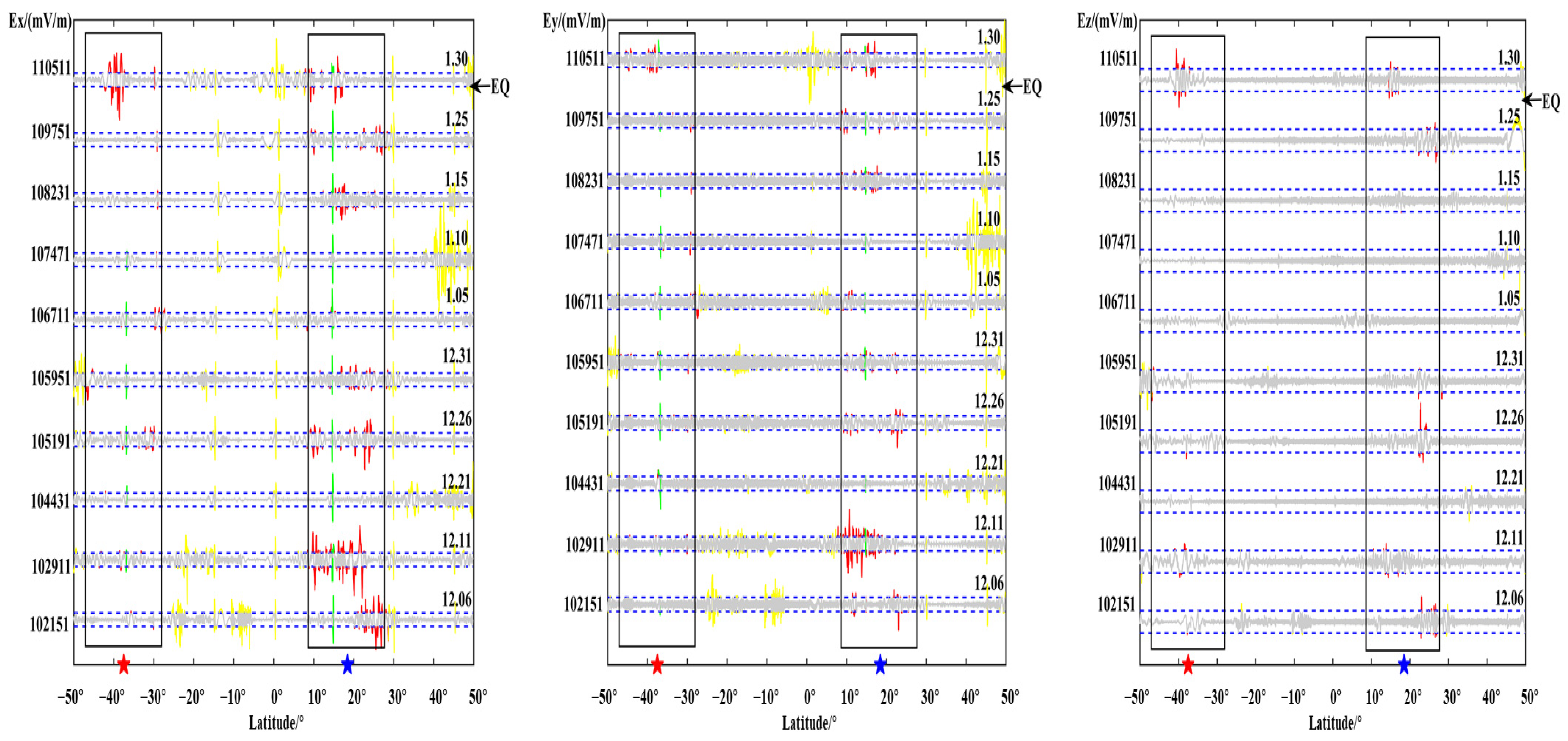
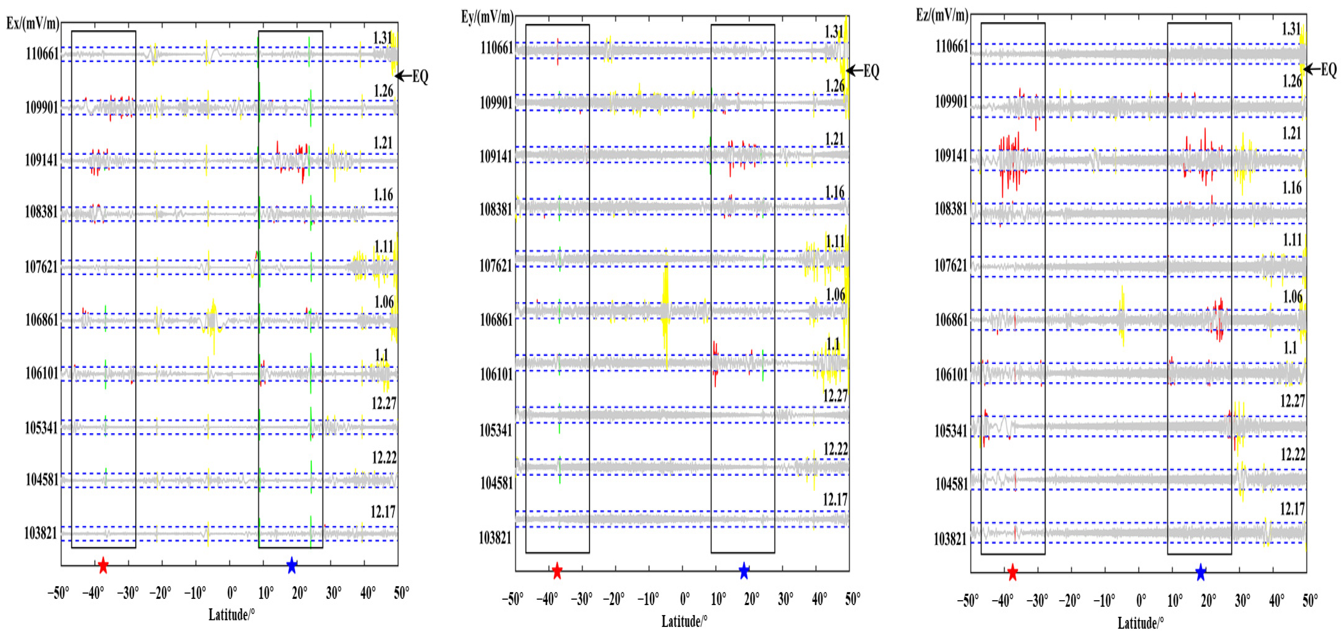
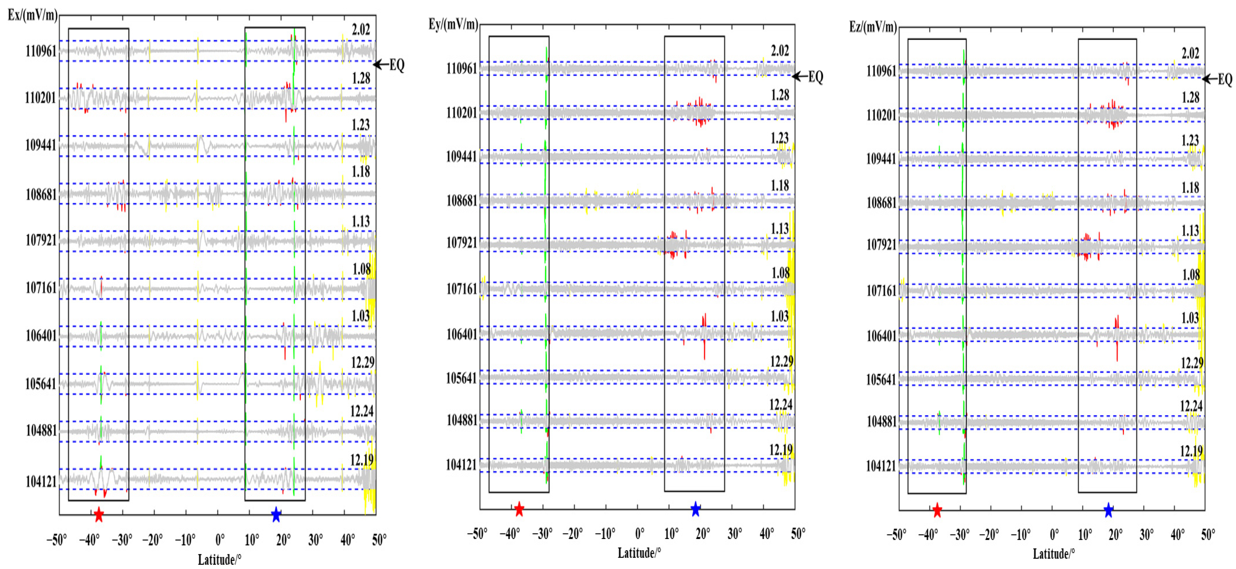
3.1. Extraction of Abnormal Information from Residual Sequence

S–G filtering is used to denoise the six pre-earthquake orbits to obtain the residual sequence without the electric field trend. Combined with the spatial trajectory and the map of the epicenter and magnetic conjugate area, the small-scale residual disturbance waveform after the removal of electric field trend is drawn. Analyzing each residual sequence shows that: (1) From the perspective of the residual amplitude, the maximum amplitude of 109,601 and 110,211 is 0.5 mV/m, which are concentrated in 20° S~0° and 10° S~0°, followed by 109,901, which changes the amplitude to 0.1 mV/m, distributed in the range of 48° S~20° N, and the other tracks 109,751, 110,051, and 110,201 have smaller amplitudes. The perturbation of the 109,751 orbit is distributed in the range of 8° N~10° N and 10° S~0°, 110,051 is distributed in the range of 10° N~20° N and 20° S~0°, and 110,201 is distributed in the range of 8° N~10° N. (2) Judging from the position of the six tracks relative to the epicenter, the large ones are on the west and middle sides, and the distances are farther, while the small ones are above and to the east of the epicenter. (3) On each track, the overall characteristics of the three components of X, Y, and Z are similar, and the electric field value changes are different.
Here, the residual sequence of the 109,751 orbit which is the closest to the epicenter on January 25 is selected for display. As shown in Figure 3 below, the residual amplitude is about 0.1 mV/m, and the abnormal changes are concentrated in the 5~15° latitude range to the south of the epicenter and within 15 degrees south of the equator; the overall characteristics of the changes of the three components are consistent, but the electric field value of the Z component is different from the X and Y components.
The wavelet analysis method is used to further analyze the disturbance, the residual data are converted to the frequency domain for analysis, and the wavelet time-frequency diagram is drawn, as shown in Figure 4. Observing Figure 4, we get: (1) From the perspective of the signal enhancement amplitude and the changes of the three components at the same latitude, the changes after the wavelet analysis of each orbit are basically the same as the residual signal. (2) From the frequency domain signal of the epicenter, 110,051 and 110,211 showed sharper enhancement changes in the frequency domain than the residual signal, and continuous signal jumps higher than other latitudes that appeared at the position above the epicenter. The frequency domain of 3~20 Hz has a disturbance change above 0.04 Hz, which is consistent with the above processing results. Wavelet time-frequency analysis converts the time-domain signal to the frequency domain, provides the energy characteristics of the waveform signal, further amplifies the signal disturbance in the epicenter, and effectively characterizes the change of the signal in the frequency and time domains which provides supplementary information in the frequency domain for variation of the residual signal at the epicenter.

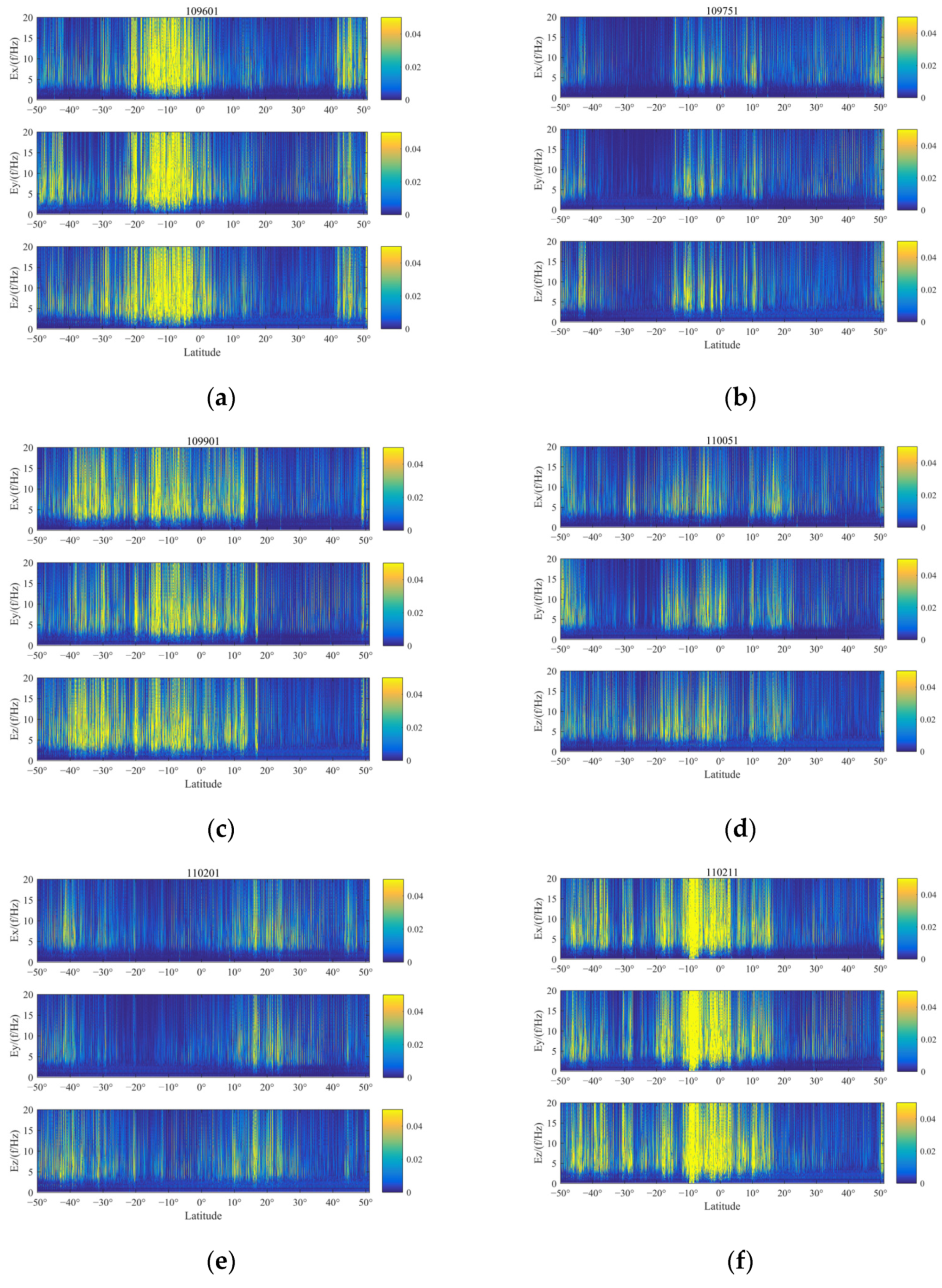
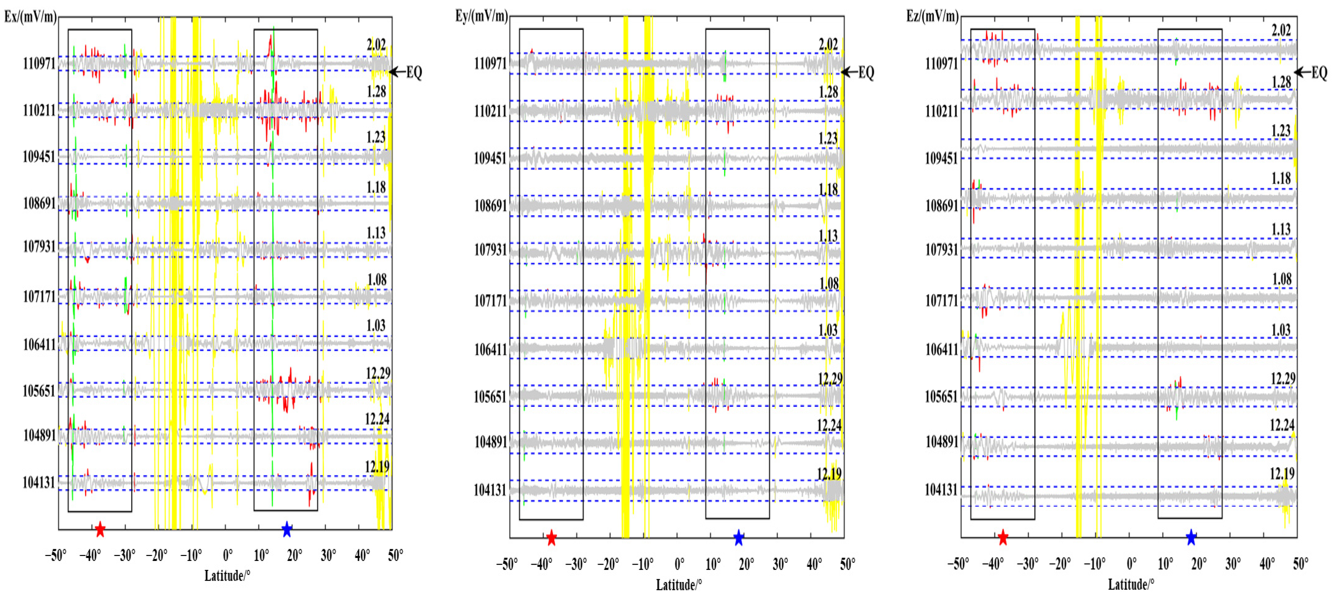
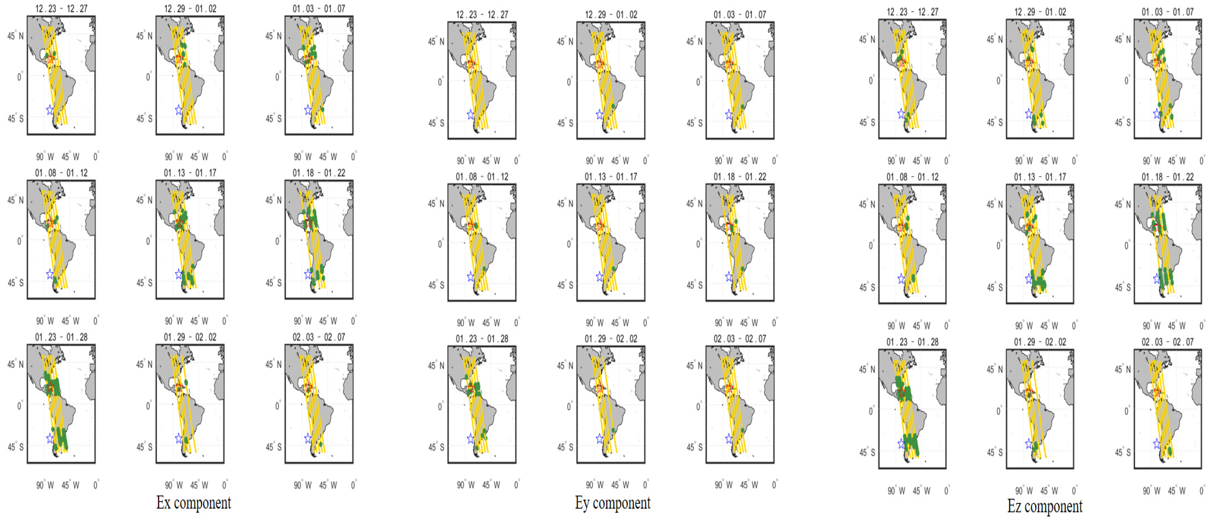
3.2. Extraction of Disturbance Signal Based on EMD

In order to further study and verify the waveform disturbance changes, one must adaptively extract the principal components of the electric field signal, and decompose the X, Y, and Z components of each track based on the EMD empirical mode decomposition algorithm, and obtain several inherent modal components (IMF). Taking the 109,751 orbit as an example, the three-component signal is decomposed by EMD to obtain several inherent modal components, and the sample entropy of each component and the average value of the sample entropy of the original signal are calculated, as shown in Table 1.
It can be seen from Table 1 that among the decomposed signals of the three components of Ex, Ey and Ez, the IMF larger than the mean value of the sample entropy is IMF1–9. Because of the large amount of information it may carry, IMF1–9 is selected for signal reconstruction to obtain more significant signal changes. The original signal and the reconstructed signal are shown in Figure 5. Compared with the original signal, the reconstructed signal removes the electric field trend and extracts the change value of the electric field more clearly. The analysis shows that the Z component in 15° N~25° N has a large abnormal jump.
In order to verify the correlation between the disturbance extracted in 4.1 and the earthquake in southern Cuba, and avoid contingency caused by studying a single track, the six pre-earthquake orbits mentioned above and their revisited orbits two months before the earthquake are selected to observe their reconstruction. The changes of the signal during the seismogenic process are shown in Figure 6, Figure 7, Figure 8, Figure 9, Figure 10 and Figure 11. The reconstructed signal after decomposition amplifies the changes in detail, which can more clearly identify the evolution and disturbance process of the ULF signal in the epicenter.
The standard deviation can reflect the degree of discrete changes in the data set. In order to more clearly identify the abnormal signals that occurred before the earthquake, the threshold value is dynamically selected linearly according to the fluctuation of the standard deviation of the orbit signal itself, and then used as the judging standard of whether the electric field waveform signal has abnormal disturbances.
Due to the complexity and diversity of space environment, signals caused by other noise interference are ignored in this study, and only signals that may be related to earthquakes are marked in red. Analyzing the reconstructed signal of each orbit, it is found that multiple component data have pulsed interference in the form of a fixed period, and the distribution is relatively uniform. This is consistent with the characteristics of the calibration signal in the DEMETER satellite. Therefore, it is believed that this periodic disturbance change is due to the interference caused by the calibration signal, and is marked in green here; besides, there are more severe interference characteristics near the north and south poles, and some signal changes are also found near 10° south latitude. According to Section 2.3, there is no impact from space magnetic storm interference, so the influence of interference may therefore be caused by the signal change of the electric field sensor itself. After excluding signals at the epicenter and its conjugate vicinity, which can be confirmed to be irrelevant to the earthquake, the other interferences are uniformly marked as yellow, and only the epicenter and its conjugate area, that is, the change of the red signal, are focused.
We select the revisited orbit of the 109,601 orbit (from the 103,521 orbit on 15 December to the 110,361 orbit after the earthquake on 29 January) and observe the seismogenic changes of the 10 orbital signals. It can be found that the three components are relatively equable in the background period of December. There was a short jump in the X and Z components at the epicenter on 25 December; significant fluctuating signals appeared at the magnetic conjugation point on 14 and 19 January, respectively, and the changes were the most significant on the 24th. After the earthquake, the signal disturbance weakened. There is a signal of small amplitude between 10° and 20° south of the epicentral area, but its amplitude is basically smaller than the magnitude of the disturbance before the earthquake.
Observing the changes in the orbit of the revisited 109,751, it can be seen that all the X and Y components of the revisited 109,751 were disturbed on 6, 11 and 26 December in the epicenter area, and the Z component between 20° and 30° north of the epicenter has slight variation before the earthquake. January was relatively calm, until the 108,231 and 10,975 orbits changed significantly at the epicenter within 15 days before the earthquake, and the disturbance continued until after the earthquake on 30 January.
Observing all the revisited orbits of 109,901 in Figure 8, it was found that the 109,901 orbit was relatively equable during the background period in December, and there was no disturbance. Only a small disturbance occurred near 10° N on January 1st, and it was over the epicenter and magnetic field on 21 January. The three components above the conjugation zone all have large fluctuations, and the three components above the epicenter and conjugation zone all have large fluctuations on 21 January with the Z component changing the most. The 110,661 orbit on 31th January after the earthquake was relatively calm, with no outliers out of bounds.
Since the post-earthquake orbit of the 110,051 orbit is missing, only the revisited orbit’s time change signal sequence from 18 December is displayed. It can be seen from Figure 9 that the epicenter area was relatively calm at the background value in December. There was a disturbance change on 2 January, after calm was restored, on 27 January before the earthquake, all three components showed obvious transboundary changes, and the Z component had a slight change on 18 December; the conjugate area manifested more prominently in the Z component, and the changed signals were mainly concentrated on 2, 12 and 17 January.
Observing 110,201 and its revisited orbits, it is found that the X component changes were relatively equable. On 13 January, the Y and Z components changed slightly. On 28, the three components were significantly disturbed over the epicenter; on 18 and 28 January, there was a small disturbance in the magnetic conjugation area; on 2 February, the 110,961 orbit after the earthquake became calm.
Figure 11 shows 110,211 and its revisited orbit. In December, the background value of its Y component was similar to that of 109,901 orbit. There was a “quiet” phenomenon. On the 28th, all three components above the epicenter area had significant fluctuations above the threshold. A large jump change too place; the changes in the magnetic conjugation area are the most obvious in the X and Z components.
The above figures show the evolution of the three components of each orbit over time. Observing its changes, most of the pre-earthquake orbits showed a certain degree of disturbance changes in the vicinity of the seismogenic zone, which is consistent with the results obtained by the above S–G filtering combined with wavelet analysis. Observing the above figure comprehensively, the temporal and spatial changes of the electric field signal can be summarized as: within one month before the earthquake, the revisited orbit had obvious enhanced disturbances at the epicenter position, and some signal disturbances shifted to the equator. The signal appeared after the earthquake and gradually returned to the form of the calm period before the earthquake. At the same time, it is found that, compared with wavelet time-frequency analysis, EMD can more clearly amplify the changes near the epicenter and provide a more detailed description of the epicenter data.
The disturbance after extraction of each orbit is plotted as a spatial change diagram, as shown in Figure 12.
A map of the temporal and spatial evolution of the two months before the earthquake is drawn. In the form of a 5-day revisit cycle, the abnormal points in the orbit exceeding the threshold are drawn in green scattered points near the earthquake area, and the yellow points are of normal values. It can be seen from Figure 12 that as time passes, the background appears to be in a calm state. As the time of the earthquake is approaching, the abnormal value gradually increases in the epicenter position. The disturbance variation is particularly severe in the 15 days before the earthquake. The spatial and temporal location manifesting characteristics of the abnormal pre-earthquake variation points of the three components are not completely consistent.

4. Discussion

The periodic characteristics of the revisited orbit provide a basis for studying the changes in the space electric field disturbance before the earthquake. The analysis of the revisited orbit signals two months before the earthquake and five days after the earthquake reveals that the six orbits within five consecutive days before the earthquake have waveform signal variations that significantly distinguish from the revisiting orbits the normal state; the epicenter revisited within a month before the earthquake also had continuous and intermittent signal changes that exceeded the abnormality; at the same time, near the magnetic conjugate area of 38° N, there were also points of abrupt variations that exceeded the threshold of standard signals. Combining previous studies and related knowledge of seismic ionospheric coupling, it can be known that seismic ionospheric coupling mainly spreads through three ways (chemical, acoustic, electromagnetic) [36,37,38,39], of which the chemical pathway is usually through the chemical process between particles in the seismogenic zone, forming charged particles in a certain spatial range, and they interact with the ionosphere in the form of an electric field. The anomaly has a certain spatial scale and temporal duration. From this research, the continuous temporal and spatial change and disturbance of above the sea surface to the south of Cuba 5 days before the earthquake is consistent with the mode of function of the chemical pathway, and the phenomenon of abnormal signals appearing above the epicenter within 5 days before the earthquake is consistent with previous studies [40,41,42,43,44]. After eliminating the interference factors of space weather, and further considering that this change may be related to earthquake preparation, it is speculated that the spatial frequency signal component caused by seismic activity is increased or weakened, thereby affecting the variation of the waveform signal. In addition, the characteristics of the three components of the electric field are different, and the electromagnetic anomalies generated before the earthquake are discontinuous. It may be because it is over the sea. The sea should be considered the fourth layer into the lithosphere–atmosphere–ionosphere coupling progress.
After analysis and research, it is found that the shapes of the three components of the electric field have similar characteristics in the two features extracted, but there are certain differences on some tracks, showing an inconsistent state. The probes ab, cd, and ad on the electric field detector load represent three different directions, the electric potential difference will change with the trajectory of the spaceflight, and the distance to the epicenter position is different when flying through different orbits, so different electric potential differences are produced. It may be that the structure of electric field detection is not uniform, which causes the three-component signal to be inconsistent. It is hard to judge directly the connection between the changes and events when the mechanism is unconfirmed. Now what we can do is to exclude other factors and then we could make the correlation with a high confidence level.
In terms of data processing methods, the two methods have different recognition of the amount of information in the waveform data. The method of residual with wavelet time-frequency analysis supplements the characteristics of the signal in the frequency domain, and its position in the epicenter can reflect the anomaly variation of the signal energy increase, but also contains high-frequency information from other regions, which is difficult to distinguish; the EMD method uses reconstructed signal to better remove the electric field trend of the original signal, and the reconstructed signal contains more information, portrays the variation of the signal from the perspective of the time domain, clearly reflects the change of amplitude of the signal in the epicenter area, and can find subtle changes related to the epicenter in the EMD reconstructed signal. The two methods recognize the characteristics of the signal from the time and frequency domain, respectively, which can more fully characterize the frequency change trend and signal details of the pre-earthquake signal, and have a better recognition effect for identifying the abnormal signal before the earthquake. However, the current research on further fusion of the two methods is still insufficient, and the selection of outliers is only based on the standard deviation of the data itself. The full fusion of the model and the setting of dynamic thresholds need to be discussed in depth based on subsequent research.

5. Conclusions

Using the ULF-band waveform of electric field Ex, Ey, and Ez data recorded by the ZH-1 satellite, the disturbance characteristics before the M7.7 earthquake that occurred in southern Cuba were studied, and the time-frequency analysis of the revisited orbit data in multiple periods before the earthquake was carried out. The conventional method of extracting small-scale waveforms was combined with wavelet time-frequency analysis for feature extraction. At the same time, the disturbance feature was extracted by the EMD empirical mode decomposition method. The extraction results of the two methods were analyzed, compared and verified, effectively achieving the extraction of the characteristics of the spatial electric field disturbance before the earthquake.
After the above feature extraction and analysis, the following conclusions are obtained:
(1)
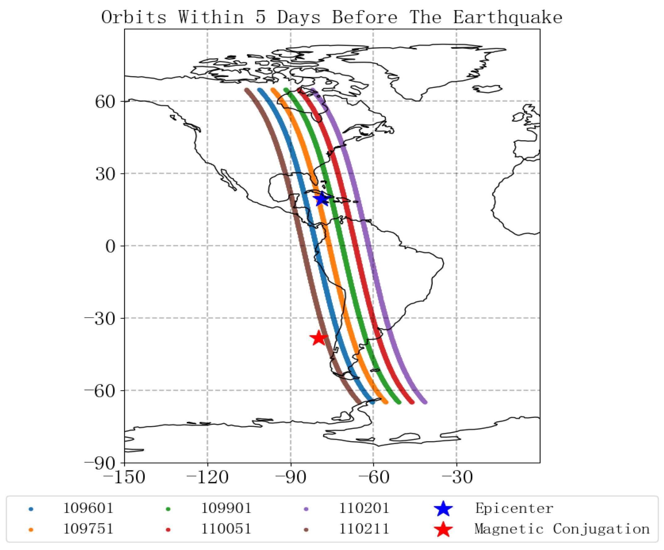
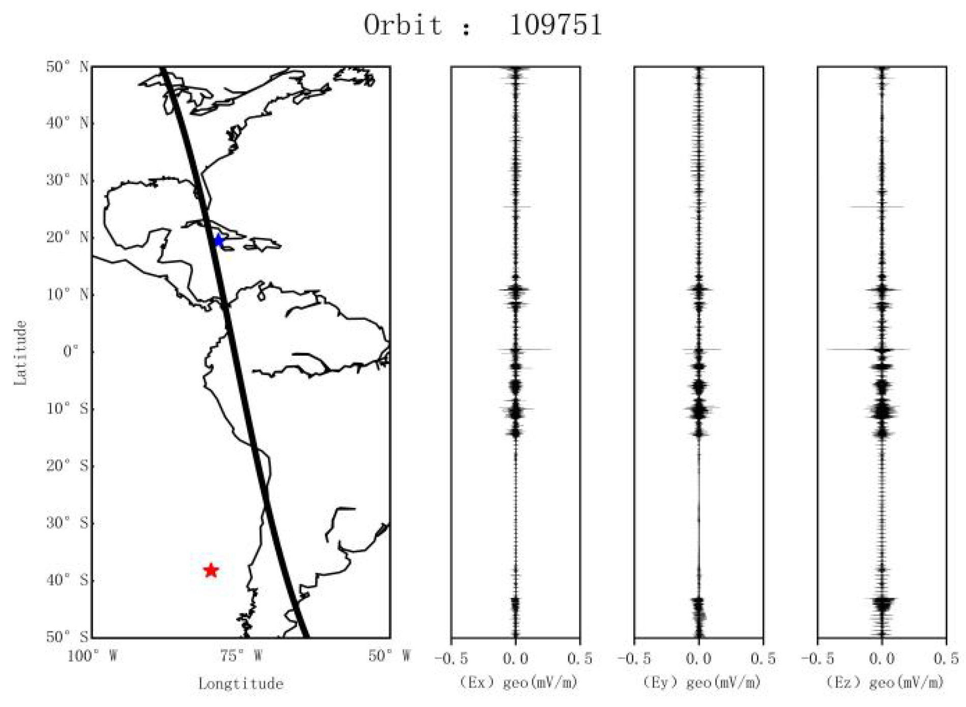
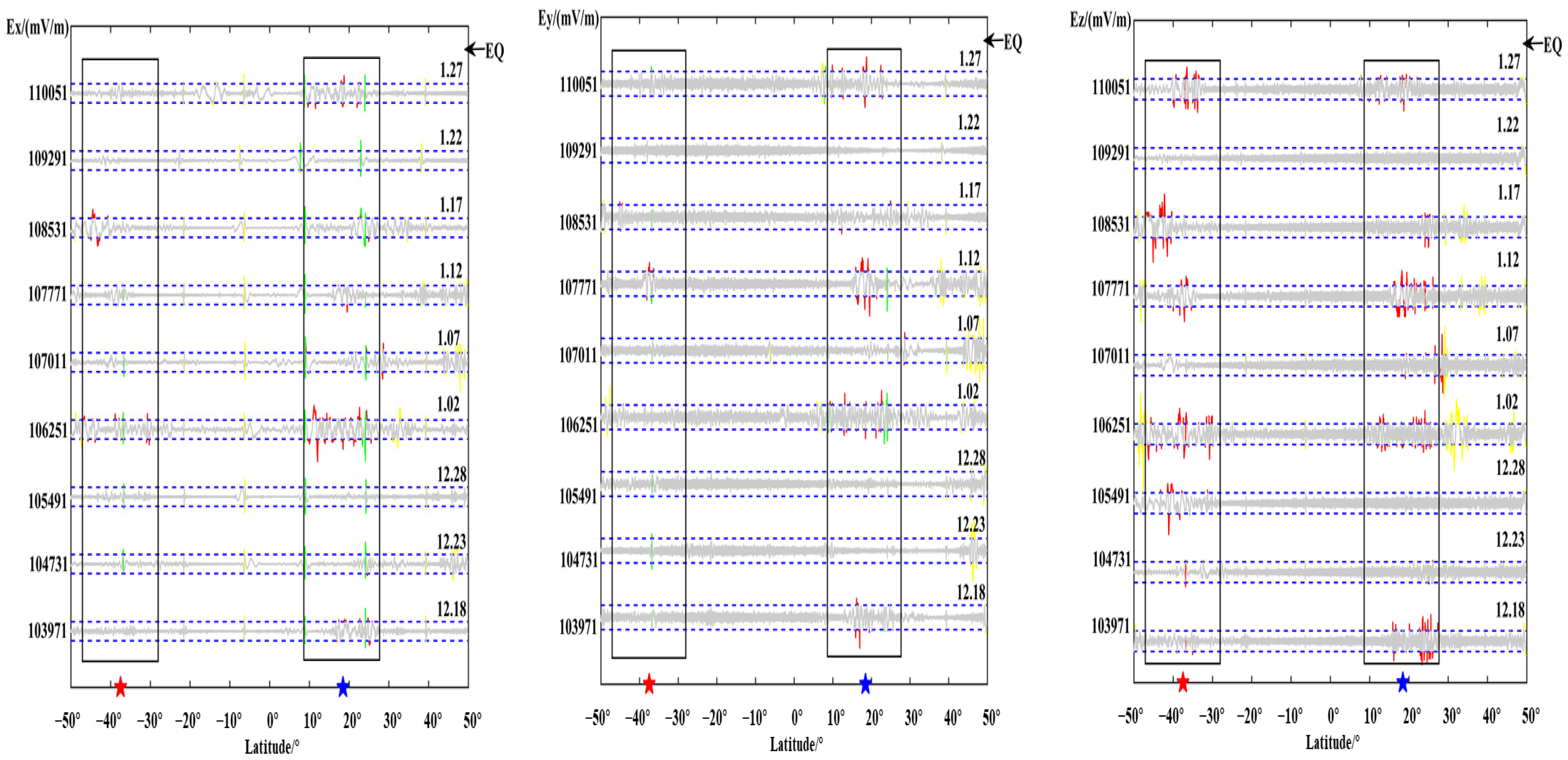
Before the earthquake in southern Cuba, the abnormal ULF signal can be observed near the epicenter, which is manifested as an increase or attenuation of the signal before the earthquake. This may be a waveform disturbance caused by the change of the frequency component of the space radiation signal caused by the earthquake.
(2)
The spatial distribution range of the disturbance is mostly concentrated in the epicentral area (10° N~20° N), but there is also a phenomenon that the disturbance signal shifts to the equator; the disturbance of the conjugate area is most obvious on the data from the orbits on the west and east side of the seismogenic zone close to the epicenter.
(3)
The signal after the three-component decomposition of the electric field waveform has good synchronization in the epicentral disturbance area, but there are certain overall shape differences.

Author Contributions

Conceptualization and methodology, Z.L.; algorithm implementation, J.L.; data analysis and conclusion, J.H.; software and investigation, J.J.; writing—review and editing, H.Y. All authors have read and agreed to the published version of the manuscript.

Funding

This research was funded by National Key R&D program (2018YFC1503501); APSCO Earthquake Project: Phase II;ISSI-BJ2019.

Institutional Review Board Statement

Not applicable.

Informed Consent Statement

Not applicable.

Data Availability Statement

Publicly available datasets were analyzed in this study. The CSES satellite electric field data can be found here: (www.leos.ac.cn, accessed on 1 September 2020). The geomagnetic index data can be found here: (http://wdc.kugi.kyoto-u.ac.jp/dstae/index.html, accessed on 1 September 2020).

Acknowledgments

This work made use of the data from the CSES mission, a project funded by China National Space Administration (CNSA) and the China Earthquake Administration (CEA). Thanks to the CSES satellite team for the data (www.leos.ac.cn, accessed on 1 September 2020). Thanks to Zhang Xuemin of the Institute of Earthquake Prediction, CEA and reviewers for the advice and suggestion.

Conflicts of Interest

The authors declare no conflict of interest.

References

  1. Ye, Q.; Fan, Y.; Du, X.B.; Cui, T.F.; Zhou, K.C.; Singh, R.P. Diurnal characteristics of geoelectric fields and their changes associated with the Alxa Zuoqi MS5.8 earthquake on 15 April 2015 (Inner Mongolia). Earthq. Sci. 2018, 31, 35–43. [Google Scholar] [CrossRef]
  2. Li, M.; Lu, J.; Zhang, X.; Shen, X. Indications of Ground-based Electromagnetic Observations to A Possible Lithosphere–Atmosphere–Ionosphere Electromagnetic Coupling before the 12 May 2008 Wenchuan MS8.0 Earthquake. Atmosphere 2019, 10, 355. [Google Scholar] [CrossRef] [Green Version]
  3. Liu, J.; Wan, W.X.; Huang, J.P.; Zhang, X.M.; Zhao, S.F.; Ouyang, X.Y.; Zeren, Z. Electron density perturbation before Chile M8.8 earthquake. Chin. J. Geophys. 2011, 54, 2717–2725. (In Chinese) [Google Scholar] [CrossRef]
  4. Namgaladze, A.; Karpov, M.; Knyazeva, M. Seismogenic Disturbances of the Ionosphere during High Geomagnetic Activity. Atmosphere 2019, 10, 359. [Google Scholar] [CrossRef] [Green Version]
  5. Ouyang, X.Y.; Zhang, X.M.; Shen, X.H.; Huang, J.P.; Liu, J.; Zeren, Z.; Zhao, S.F. Disturbance of O+ densitybefore major earthquake detected by DEMETER satellite. Chin. J. Space Sci. 2011, 31, 607–617. [Google Scholar]
  6. Chen, C.-H.; Sun, Y.-Y.; Lin, K.; Liu, J.; Wang, Y.; Gao, Y.; Zhang, D.; Xu, R.; Chen, C. The LAI Coupling Associated with the M6 Luxian Earthquake in China on 16 September 2021. Atmosphere 2021, 12, 1621. [Google Scholar] [CrossRef]
  7. Henderson, T.R.; Sonwalkar, V.S.; Helliwell, R.A.; Inan, U.S.; Fraser-Smith, A.C. A search for ELF/VLF emissions induced by earthquakes as observed in the ionosphere by the DE 2 satellite. J. Geophys. Res. Space Phys. 1993, 98, 9503–9514. [Google Scholar] [CrossRef]
  8. Yan, R.; Parrot, M.; Pinçon, J.-L. Statistical Study on Variations of the Ionospheric Ion Density Observed by DEMETER and Related to Seismic Activities. J. Geophys. Res. Space Phys. 2017, 122, 12421–12429. [Google Scholar] [CrossRef] [Green Version]
  9. Hayakawa, M.; Hattori, K.; Ohta, K. Monitoring of ULF (ultra-low-frequency) geomagnetic variations associated with earthquakes. Sensors 2007, 7, 1108–1122. [Google Scholar] [CrossRef] [Green Version]
  10. Febriani, F.; Ahadi, S.; Anggono, T.; Dewi, C.N.; Prasetio, A.D. Applying Wavelet Analysis to Assess the Ultra Low Frequency (ULF) Geomagnetic Anomalies prior to the M6.1 Banten Earthquake (2018). IOP Conf. Ser. Earth Environ. Sci. 2021, 789, 012064. [Google Scholar] [CrossRef]
  11. Fenoglio, M.A.; Johnston, M.J.S.; Byerlee, J.D. Magnetic and electric fields associated with changes in high pore pressure in fault zones: Application to the Loma Prieta ULF emissions. J. Geophys. Res. Solid Earth 1995, 100, 12951–12958. [Google Scholar] [CrossRef]
  12. Zhao, S.F.; Liao, L.; Zhang, X.M. Trans-ionospheric VLF wave power absorption of terrestrial VLF signal. Chin. J. Geophys. 2017, 60, 3004–3014. (In Chinese) [Google Scholar] [CrossRef]
  13. Jiadong, Q.; Qinzhong, M.; Shaonong, L. Further study on the anomalies in apparent resistivity in the NE configuration at Chengdu station associated with Wenchuan Ms8,0 earthquake. Acta Sismol. Sin. 2012, 35, 4–17. [Google Scholar]
  14. Pulinets, S.; Boyarchuk, K. Ionospheric Precursors of Earthquakes. In Ionospheric Precursors of Earthquakes; Springer: Berlin/Heidelberg, Germany, 2005. [Google Scholar] [CrossRef]
  15. Varotsos, P.; Alexopoulos, K.; Nomicos, K.; Lazaridou, M. Earthquake prediction and electric signals. Nature 1986, 322, 120. [Google Scholar] [CrossRef]
  16. Ouyang, X.Y.; Parrot, M.; Bortnik, J. ULF Wave Activity Observed in the Nighttime Ionosphere above and Some Hours before Strong Earthquakes. J. Geophys. Res. Space Phys. 2020, 125, e2020JA028396. [Google Scholar] [CrossRef]
  17. Ouyang, X.Y.; Shen, X.H. A method for pre-processing UL.F electric field disturbances observed by DEMETER and its case application analysis. Acta Seismol. Sin. 2015, 37, 820–829. [Google Scholar] [CrossRef]
  18. Ouyang, X.Y.; Shen, X.H. The interference analysis of ULF electric field waveform observed by DEMETER satellite. Seismol. Geomagn. Obs. Res. 2015, 36, 19–25. [Google Scholar]
  19. Zeren, Z.M.; Shen, X.H.; Cao, J.B.; Zhang, X.M.; Huang, J.P.; Liu, J.; Ouyang, X.Y.; Zhao, S.F. Statistical analysis of EL.F/VLF magnetic field disturbances before major earthquakes. Chin. J. Geo. Phys. 2012, 55, 3699–3708. (In Chinese) [Google Scholar] [CrossRef]
  20. Zeren, Z.; Zhang, X.; Liu, J.; Ouyang, X.; Xiong, P.; Shen, X. Using DEMETER satellite LANGMIUR probe observation data to study ionospheric disturbances before strong earthquakes. Seismol. Geol. 2010, 32, 424–433. [Google Scholar]
  21. Shen, X.H.; Zhang, X.M.; Yuan, S.G.; Wang, L.W.; Cao, J.B.; Huang, J.P.; Zhu, X.H. Piergiorgio, P.; Dai, J.P. The state-of-the-art of the China Seismo-Electromagnetic Satellite mission. Sci. Chin. Technol. Sci. 2018, 61, 634–642. [Google Scholar] [CrossRef]
  22. Huang, J.P.; Shen, X.H.; Zhang, X.M.; Lu, H.X.; Tan, Q.; Wang, Q.; Yan, R.; Chu, W.; Yang, Y.Y.; Liu, D.P.; et al. Application system and data description of the China Seismo-Electromagnetic Satellite. Earth Planet. Phys. 2018, 2, 444–454. [Google Scholar] [CrossRef]
  23. Cao, B.N.; Ge, Z.X. 2020 Mw7.7 Caribbean Sea earthquake: A supershear event revealed by teleseismic P wave back-projection method. Chin. J. Geo. Phys. 2021, 64, 1558–1568. (In Chinese) [Google Scholar] [CrossRef]
  24. Li, M. The Statistical Characteristics of Seismic Ionospheric Anomalies and the Study of Earth-Atmosphere Electromagnetic Coupling based on the Wenchuan M_S8.0 Earthquake. Ph.D. Thesis, China University of Geosciences: Beijing, China, 2015. [Google Scholar]
  25. Huang, J.P.; Lei, J.G.; Li, S.X.; Zeren, Z.M.; Li, L.; Zhu, X.H.; Yu, W.H. The Electric Field Detector(EFD) onboard the ZH-1 satellite and first observational results. Earth Planet. Phys. 2018, 2, 469–478. [Google Scholar] [CrossRef]
  26. Ma, M.J.; Li, C.; Lei, J.G.; Li, S.X.; Wang, R.F.; Zong, C.; Liu, Z.; Chen, T.; Cui, Y. Experimental study on ZH-1SEFD for CSES in the ground simulating plasma environments. Planet. Space Sci. 2020, 192, 105006. [Google Scholar] [CrossRef]
  27. Diego, P.; Bertello, I.; Candidi, M.; Mura, A.; Coco, I.; Vannaroni, G.; Ubertini, P.; Badoni, D. Electric field computation analysis for the Electric Field Detector (EFD) on board the China Seismic-Electromagnetic Satellite (CSES). Adv. Space Res. 2017, 60, 2206–2216. [Google Scholar] [CrossRef]
  28. Dobrovolsky, I.P.; Zubkov, S.I.; Miachkin, V.I. Estimation of the size of earthquake preparation zones. Pure Appl. Geophys. PAGEOPH 1979, 117, 1025–1044. [Google Scholar] [CrossRef]
  29. Xu, W. Geomagnetism; Seismological Press: Beijing, China, 2003; pp. 288–296. [Google Scholar]
  30. Quan, Q.; Cai, K.Y. Time-domain analysis of the Savitzky–Golay filters. Digit. Signal Process. 2012, 22, 238–245. [Google Scholar] [CrossRef]
  31. Han, B. Wavelet Transform and Its Application in Seismic Electromagnetic Signal Analysis. Master’s Thesis, Institute of Geology, China Earthquake Administration: Beijing, China, 2014. [Google Scholar]
  32. Han, P.; Hattori, K.; Huang, Q.; Hirano, T.; Ishiguro, Y.; Yoshino, C.; Febriani, F. Evaluation of ULF electromagnetic phenomena associated with the 2000 Izu Islands earthquake swarm by wavelet transform analysis. Nat. Hazards Earth Syst. Sci. 2011, 11, 965–970. [Google Scholar] [CrossRef] [Green Version]
  33. Liu, J.; Gu, Y.; Chou, Y.; Gu, J. Seismic data random noise reduction using a method based on improved complementary ensemble EMD and adaptive interval threshold. Explor. Geophys. 2021, 52, 137–149. [Google Scholar]
  34. Lu, J.; Wang, Z. The Systematic Bias of Entropy Calculation in the Multi-Scale Entropy Algorithm. Entropy 2021, 23, 659. [Google Scholar] [CrossRef]
  35. Richman, J.S.; Moorman, J.R. Physiological time-series analysis using approximate entropy and sample entropy. Am. J. Physiology. Heart Circ. Physiol. 2000, 278, H2039–H2049. [Google Scholar] [CrossRef] [PubMed] [Green Version]
  36. Spogli, L.; Sabbagh, D.; Regi, M.; Cesaroni, C.; Perrone, L.; Alfonsi, L.; Di Mauro, D.; Lepidi, S.; Campuzano, S.A.; Marchetti, D.; et al. Ionospheric Response Over Brazil to the August 2018 Geomagnetic Storm as Probed by CSES-01 and Swarm Satellites and by Local Ground-Based Observations. J. Geophys. Res. Space Phys. 2021, 126, e2020JA028368. [Google Scholar] [CrossRef]
  37. Li, M.; Shen, X.; Parrot, M.; Zhang, X.; Zhang, Y.; Yu, C.; Yan, R.; Liu, D.; Lu, H.; Guo, F.; et al. Primary Joint Statistical Seismic Influence on Ionospheric Parameters Recorded by the CSES and DEMETER Satellites. J. Geophys. Res. Space Phys. 2020, 125, e2020JA028116. [Google Scholar] [CrossRef]
  38. Kuo, C.L.; Huba, G.; Joyce, G.; Lee, L.C. Ionosphere plasma bubbles and density variations induced by pre-earthquake rock currents and associated surface charges. J. Geophys. Res. Space Phys. 2011, 116, A10317. [Google Scholar] [CrossRef] [Green Version]
  39. Kuo, C.L.; Lee, L.C.; Huba, J.D. An improved coupling model for the lithosphere-atmosphere-ionosphere system. J. Geophys. Res. Space Phys. 2014, 119, 3189–3205. [Google Scholar] [CrossRef]
  40. Zeren, Z.M.; Hu, Y.; Shen, X.; Chu, W.; Piersanti, M.; Parmentier, A.; Zhang, Z.; Wang, Q.; Huang, J.; Zhao, S.; et al. Storm-Time Features of the Ionospheric ELF/VLF Waves and Energetic Electron Fluxes Revealed by the China Seismo-Electromagnetic Satellite. Appl. Sci. 2021, 11, 2617. [Google Scholar]
  41. Gokhberg, M.B.; Pilipenko, V.A.; Pokhotelov, O.A. Satellite observation of the electromagnetic radiation above the epicentral region of an incipient earthquake. Dokl. Acad. Sci. USSR Earth Sci. Ser. 1983, 268, A76-43596. [Google Scholar]
  42. Serebryakova, O.N.; Bilichenko, S.V.; Chmyrev, V.M.; Parrot, M.; Rauch, J.L.; Lefeuvre, F.; Pokhotelov, O.A. Electromagnetic ELF radiation from earthquake regions as observed by low-altitude satellites. Geophys. Res. Lett. 2013, 19, 91–94. [Google Scholar] [CrossRef]
  43. Parrot, M. Statistical analysis of the ion density measured by the satellite DEMETER in relation with the seismic activity. Earthq. Sci. 2011, 24, 513–521. [Google Scholar] [CrossRef] [Green Version]
  44. Bhattacharya, S.; Sarkar, S.; Gwal, A.K.; Parrot, M. Electric and magnetic field perturbations recorded by DEMETER satellite before seismic events of the 17th July 2006 M 7.7 earthquake in Indonesia. J. Asian Earth Sci. 2009, 34, 634–644. [Google Scholar] [CrossRef]
Figure 1. Satellite trajectory projection within 5 days before the earthquake (the blue star is the epicenter, the red is the epicenter magnetic conjugate point).
Atmosphere 13 00179 g001
Figure 2. Changes of ∑Kp and Dst index in the selected study period of the sample earthquake.
Atmosphere 13 00179 g002
Figure 3. The residual waveform of the 109,751 orbit before the earthquake (the blue and red marks in the figure represent the epicenter and its magnetic conjugate point, respectively).
Atmosphere 13 00179 g003
Figure 4. Three-component wavelet time-frequency analysis diagram of electric field before earthquake. (a) Orbit of 109,601; (b) orbit of 109,751; (c) orbit of 109,901; (d) orbit of 110,051; (e) orbit of 110,201; (f) orbit of 110,211.
Atmosphere 13 00179 g004
Figure 5. Original signal and reconstructed signal of 109,751 track. (a) Original signal; (b) reconstructed signal.
Atmosphere 13 00179 g005
Figure 6. Orbit 109,601 and its revisited tracks (the red and blue five-pointed stars indicate the magnetic conjugate and epicenter positions, respectively, and the black frame indicates the seismogenic range where disturbance signals may exist, the horizontal blue dotted line is the threshold set according to the standard deviation of the electric field signal after reconstruction, respectively; the following figures same as here noted).
Atmosphere 13 00179 g006
Figure 7. Orbit 109,751 and its revisited tracks.
Atmosphere 13 00179 g007
Figure 8. Orbit 109,901 and its revisited tracks.
Atmosphere 13 00179 g008
Figure 9. Orbit 110,051 and its revisited tracks.
Atmosphere 13 00179 g009
Figure 10. Orbit 110,201 and its revisited tracks.
Atmosphere 13 00179 g010
Figure 11. Orbit 110,211 and its revisited tracks.
Atmosphere 13 00179 g011
Figure 12. The time-space evolution of the orbit.
Atmosphere 13 00179 g012
Table 1. Sample entropy and its mean value of each IMF of 109,751.
MeanIMF1IMF2IMF3IMF4IMF5IMF6IMF7IMF8IMF9IMF10IMF11IMF12IMF13
Ex2.8363.70243.72173.77653.80103.70853.66183.70323.30603.14532.36801.34830.61470.0118
Ey2.9923.78433.71503.79093.78833.72653.51133.10463.27423.40462.47851.33040.0005
Ez3.0733.71783.75453.68683.72533.77543.45373.22643.32223.26031.86390.0122
Publisher’s Note: MDPI stays neutral with regard to jurisdictional claims in published maps and institutional affiliations.

