
PCA-Based Identification of Built Environment Factors Reducing PM2.5 Pollution in Neighborhoods of Five Chinese Megacities

School of Architecture & Urban Planning, Huazhong University of Science and Technology, Wuhan 430074, China
*
Author to whom correspondence should be addressed.
Atmosphere 2022, 13(1), 115; https://doi.org/10.3390/atmos13010115
Submission received: 29 November 2021
/
Revised: 6 January 2022
/
Accepted: 10 January 2022
/
Published: 12 January 2022
(This article belongs to the Special Issue Air Pollution in China)
Abstract
:Air pollution, especially PM2.5 pollution, still seriously endangers the health of urban residents in China. The built environment is an important factor affecting PM2.5; however, the key factors remain unclear. Based on 37 neighborhoods located in five Chinese megacities, three relative indicators (the range, duration, and rate of change in PM2.5 concentration) at four pollution levels were calculated as dependent variables to exclude the background levels of PM2.5 in different cities. Nineteen built environment factors extracted from green space and gray space and three meteorological factors were used as independent variables. Principal component analysis was adopted to reveal the relationship between built environment factors, meteorological factors, and PM2.5. Accordingly, 24 models were built using 32 training neighborhood samples. The results showed that the adj_R2 of most models was between 0.6 and 0.8, and the highest adj_R2 was 0.813. Four principal factors were the most important factors that significantly affected the growth and reduction of PM2.5, reflecting the differences in green and gray spaces, building height and its differences, relative humidity, openness, and other characteristics of the neighborhood. Furthermore, the relative error was used to test the error of the predicted values of five verification neighborhood samples, finding that these models had a high fitting degree and can better predict the growth and reduction of PM2.5 based on these built environment factors.
1. Introduction
Air pollution, especially PM2.5 pollution, still seriously endangers the health of urban residents in China. According to the 2020 World Air Quality Report published by IQAir, China is 14th in the rankings for poor air quality among the 106 countries that have been given air quality monitoring stations by the WHO. In particular, the middle and lower reaches of the Yangtze River are among of the most polluted areas in China, where a large number of residents live. Serious PM2.5 pollution has resulted in respiratory issues, asthma, and even death [1]. To maintain the basic requirement of respiratory health, it is urgent to improve air quality.
Spatial-temporal variations in PM2.5 and the impact factors on PM2.5 have attracted much attention in recent years; among these studies, PM2.5 levels were mainly affected by socioeconomic environments [2], climatic conditions [3], and urban physical environments [4]. Human activities, such as traffic emissions, industrial activities, and coal consumption, cause severe PM2.5 pollution [5,6]. At the same time, the loss of natural land and increase in artificial ground cover exacerbate the problem [7]. In addition, the change in urban land cover and its spatial pattern leads to environmental problems, especially urban heat island effects that always contribute to gathering atmospheric pollutants or forming secondary pollutants, thereby strengthening PM2.5 pollution [8]. Investigating the temporal variations in PM2.5 and its mitigation approach is essential to improve the human settlement environment.
The built environment, usually measured by factors from various perspectives including land cover type, land use, urban form at the urban scale and public space, layout of buildings and roads at the neighborhood scale [9], is one of the important factors affecting PM2.5; however, the key factors remain unclear. Obvious differences in PM2.5 levels are found across urban land cover patterns [10]. In addition, urban landscape patterns or structures, including the composition and configuration of built environments, have aroused interest by using a series of relevant metrics to investigate their effects on PM2.5 [11,12,13,14], although the influence of individual metrics may differ among studies. Moreover, urban morphology has attracted increasing attention because of its strong impacts on PM2.5. At the city scale, the spatial format of urban built-up areas, such as the size, compactness, fragmentation, and complexity of the morphology of urban areas, influences the city’s average PM2.5 level [15,16,17]. At the local scale, the PM2.5 concentration varies from neighborhood to neighborhood [18]. The difference in street canyon characteristics, building layout, and spatial form is one of the important factors that significantly influence PM2.5 levels [19,20,21]. Local climate zones (LCZs), a concept aimed at classifying local built environment features, have been widely used in urban climate studies [22,23,24]. Ten built-up LCZs and seven land cover LCZs can be provided for measuring different built environments and natural environments, respectively. Indicators, such as the sky view factor, aspect ratio, impervious surface fraction, pervious surface fraction, and height of roughness elements, are frequently used for determining these LCZs [25,26,27]. However, they are rarely involved in the PM2.5 field. Neighborhood-level PM2.5 pollution should be a main concern because it is closely related to people’s daily lives. In a high-density neighborhood environment, densely constructed buildings block air ventilation and consequently impede pollutant dispersion [28]. Particular attention should be given to the mitigation of PM2.5 by optimizing the neighborhood-level built environment, which constitutes the basic fabric in a city.
Previous studies have explored the relationship between the urban built environment and PM2.5 from different aspects, yet there are still shortcomings. First, the lack of systematic investigation of the built environment may result in the unclear key factors that significantly influence PM2.5. Second, most studies focus on individual cities instead of regions, which may limit the applicability of the research findings. Considering the complexity of the built environment in a neighborhood, traditional stepwise regression analysis has some limitations, including the potential collinearity among multiple variables and the possibility of removal of some predictive variables significantly related to dependent variables [29]. Principal component analysis (PCA) has been adopted to convert complex variables into new variables that contain most of the original information and are independent of each other, thereby reducing the predictors’ collinearity in PM2.5 simulation [30].
For this, this study explored key built environment factors influencing PM2.5 in common neighborhoods that are abundant in cities. We focused on 37 neighborhoods located in five megacities in the middle and lower reaches of the Yangtze River to better understand the influence mechanism of the built environment on PM2.5 pollution. Principal component analysis (PCA) was conducted before regression analysis to increase its performance. All principal component variables were retained for regression analysis to establish the optimal influencing factors. Therefore, key factors can be obtained.
2. Materials and Methods
2.1. Study Area and Neighborhoods
Five megacities (Wuhan, Hefei, Nanjing, Shanghai, and Hangzhou) in the middle and lower reaches of the Yangtze River were selected as the study area (Figure 1); they have the same climate conditions. Due to the extreme high-density construction, these cities experience more serious PM2.5 pollution than other cities in this region [31]. The similar features of the five cities provide sufficient comparability for this study, including urban form, landform, population, and PM2.5 pollution characteristics.
On average, each city has 10 national PM2.5 monitoring stations that present a relatively uniform distribution throughout the constructed areas. A neighborhood was then defined as a square domain with an area of 1 km2 (1 km × 1 km) centered at a monitoring station because 1 km is a common size for a neighborhood division in China and was frequently used in previous studies [32,33]. In addition, the air environment within this size plays an important role in people’s quality of daily life [34]. In consideration of the unique locations of 13 neighborhoods and subsequent special land use, such as close to pollution sources (construction sites) and natural land (urban parks or scenic regions), 37 neighborhoods were selected for analysis in this study. Detailed information on the 37 cities is shown in Table S1.
2.2. PM2.5 Data Source and Processing
Our previous studies examined the influences of neighborhood green space and urban morphology on PM2.5 separately, providing evidence for the effects of urban green space coverage and morphological patterns and gray space forms on PM2.5 [18,32,35]. As a series of studies, hourly PM2.5 concentrations from 2016 to 2017 were collected from monitoring stations to ensure the consistency of PM2.5 data. These data in different cities were monitored with the same standard. Because of the different locations of 37 neighborhoods, the uncontrolled factors (such as weather conditions, PM2.5 background concentration of five cities) were kept at similar levels to remove the external impact factors as much as possible and to greatly minimize evident differences, thereby performing an intercomparison. Consistent with our previous studies [32,35], three relative indicators, the range (Cin and Cde), duration (Δtin and Δtde), and rate (Cin’ and Cde’), of the increase and decrease in PM2.5 concentration were calculated. To investigate pollution-level differences in the effect of the neighborhood-level built environment on PM2.5, four pollution levels, including slight (PM2.5 level ranging from 75 μg/m3 to 114 μg/m3), moderate (PM2.5 level ranging from 115 μg/m3 to 150 μg/m3), heavy (PM2.5 level greater than 150 μg/m3), and overall pollution, were analyzed based on Chinese ambient air quality standards. The average of slight, moderate, and heavy pollution levels of observations was defined as the overall pollution level. The process of PM2.5 data is shown in Figure 2. Consequently, PM2.5 data of eight, three, and two days in 2016, and eight, two, and one day in 2017 were used for slight, moderate, and heavy pollution, respectively (Table S2).
2.3. Built Environment Variables and Meteorological Factors
Built environment factors, including green space and gray space, were included in this study, as well as three important meteorological factors: atmospheric temperature (Ta), relative humidity (RH), and wind velocity (V). A total of 22 variables were selected for analysis based on the quantity and spatial pattern of green and gray spaces (Table 1). Detailed information on the 22 variables is shown in Tables S3–S5. The determination of these variables also took into account their potential impacts on PM2.5 and the representativeness of built environment characteristics in neighborhoods.
The measurements and computations of built environment factors were based on a GIS vector dataset generated with a high-precision digital map (Google Earth, 2017) of each city, which ensured high accuracy of the calculation. On the one hand, the neighborhood green space cover ratio (GCR) and tree cover ratio (TCR) were two variables measuring the quantity of green space in the neighborhoods. The spatial pattern of green space was measured by morphological spatial pattern analysis (MSPA), which can provide seven types of green space patterns, including the core, islet, perforation, edge, loop, bridge, and branch [32].
On the other hand, the neighborhood hard space cover ratio (HSCR) was used as the quantity variable for gray space. Spatial pattern variables of the gray space were selected with a consideration of the density, vertical morphology, and spatial layout of gray spaces in neighborhoods. First, building density was considered one of the most important density variables, which was further classified into three categories, including building densities of one to three floors (BD_1), four to nine floors (BD_2), and more than nine floors (BD_3) [35]. In addition, as one of the major pollutant sources in neighborhoods, roads are a special kind of gray space, which may reflect the degree of traffic emissions. Road density (RD) was calculated as in many previous studies [36,37]. Second, the floor area ratio (FAR), mean building height (H), and standard deviation of building height (Hσ) were adopted to measure the vertical morphology of gray space in neighborhoods. FAR reflects the development intensity of the neighborhood. The larger the FAR is, the greater the development intensity and the higher the height of buildings. A neighborhood with a higher building height usually has a lower wind velocity near the ground, which results in better ventilation conditions [38]. Hσ represents the variation of building height. The higher the Hσ, the dispersion of the building height is greater. Third, the building evenness index (BEI) and sky view factor (SVF) were chosen to represent the layout of buildings in the neighborhood. BEI is a reflection of the difference in buildings’ flat form. A neighborhood with a higher BEI value implies a more uneven flat form of buildings. SVF is an important index reflecting built environment geometry [39]. A lower value of SVF indicates a more closed neighborhood space. The 3D building models were adopted for the calculation of SVF based on ArcGIS software according to the method of Gal’ et al. [40].
2.4. Analytical Methods
2.4.1. PCA Analysis
PCA was performed before establishing a regression model to involve all built environment factors and meteorological factors in the models as much as possible. The method can also remove the collinearity of independent variables to a certain extent. The principle of PCA is to convert a large number of factors into new principal factors through certain calculation methods and retain most of the information contained in the initial factors [41]. The principal factors are independent of each other and have no correlation, thereby eliminating the collinearity between factors when performing regression analysis. The relationship between the principal factors and the initial factors is as follows:
where Pi is the i-th principal factor, n is the number of principal factors, equal to 22, lni refers to a principal component loading of xi, and λi denotes an eigenvalue of the i-th principal factor.
Before PCA, it is necessary to carry out standardization due to the various dimensions of each factor in green space, gray space, and meteorology. The Kaiser–Meyer–Olkin (KMO) test and Bartlett sphere test were performed for 22 factors. PCA can be carried out only when the KMO value is greater than 0.5 and the Bartlett sphere test is significant (p-value < 0.01). PCA was then carried out using standardized factors. According to the number of independent variables, a total of 22 principal factors can be obtained. The variance and eigenvalue of the principal factor reflect their contribution to the initial factor. The greater the value, the greater the contribution and the information containing the initial factor.
2.4.2. Regression Models and Evaluation
As Zhai et al. [29] suggested, there may be some problems that the contributions of the predictors truly driving PM2.5 variations were unclear when using anterior principal components as explanatory variables without explicit rules and standards. To better understand the relationship between the built environment and PM2.5 and establish regression models, this study carried out stepwise regression analysis involving all principal factors, which can have a screening process for the principal factors and obtain the principal factors that have a significant impact on the dependent variables [29]. The verification of regression models was in accordance with the common methods used in relevant research fields in which the neighborhood samples were divided into test samples and verification samples [35]. The selection of two types of samples should not only consider that there are enough test samples to establish the regression model but also take a certain number of verification samples for validation. Therefore, one neighborhood sample in each city was randomly selected for validation, including WH4, HF5, NJ3, SH4, and HZ4. The remaining 32 neighborhood samples were test samples for the construction of the regression model.
The accuracy of the regression model was measured by comparing the difference between predicted values and actual values of the dependent variable. The relative error (RE) was used to evaluate the accuracy of the predicted values of the PM2.5 indicators of the five validation samples.
where REi is the relative error of the i-th validation sample and yi′ and yi are the predicted value and actual value of a PM2.5 indicator of the i-th validation sample, respectively.
3. Results and Discussion
3.1. Results of PCA
3.1.1. Overall Characteristics of PCA
PCA had pollution level differences due to the difference in meteorological factors included at the different pollution levels. At the overall pollution level, the KMO value of 22 standardized factors was 0.630, and the significance of the Bartlett spherical test was 0.000, which met the requirements of PCA. As shown in Figure 3a, with the increase in the number of principal factors, the eigenvalues and variance showed a downwards trend. The eigenvalue of principal factors reflects their contribution. The eigenvalues of the first six main factors were greater than 1, and the cumulative contribution of these six principal factors was 85.7%, which can explain most of the information of the initial factors. When the number of principal factors reached 12, it could basically contain 98% of the information of the initial factors. The contribution of the first principal factor (P1) to the total variance was 35.2%. There was little difference between the loadings of P1, most of which were between 0.2 and 0.3. P1 was negatively correlated with the green space factor and positively correlated with the gray space factor. Therefore, P1 reflects the great difference between the green space and the gray space of the neighborhood. The contribution of P2 to the total variance was 18.7%. The higher loading of P2 was higher than 0.3, which was mainly positively correlated with TCR (x1) and the Edge (x6), reflecting the large-scale green space of the neighborhood. The contribution of P3 to the total variance was 11.2%. The higher loading of P3 was more than 0.4, which was significantly positively correlated with H (x15) and Hσ (x16), reflecting the higher building height in the neighborhood and their greater height differences. P4 contributed 9.2% to the total variance. Relative humidity (x21) and wind speed (x22) were two principal factors for P4, representing meteorological factors. P5 and P6 contributed 6.4% and 5% to the total variance, respectively, and GCR (x2) and Loop (x7) were principal factors.
The variance and eigenvalue showed similar trends at different pollution levels, which were similar to those of the overall pollution (Figure 3b). The KMO values of 22 standardized factors were 0.621, 0.615, and 0.612 for slight, moderate, and heavy pollution, respectively, and the significance of the Bartlett spherical test was 0.000. The eigenvalues of the first six principal factors were greater than 1, and the cumulative contributions of these six main factors were 85.3%, 86.0%, and 83.9%. When the number of principal factors reached 12, they could contain 98% of the information of the initial factors.
3.1.2. Principal Factors Composition
The principal factor (Pi) is composed of 22 initial factors (xi) with a certain proportion coefficient (principal component loading l). The absolute value of the loading represents the contribution of the initial factor to a Pi, and the positive and negative values represent the influence mode of the initial factor on a Pi. Therefore, the principal component of a Pi is reflected by the initial factor with relatively high loadings. There were certain differences in the higher loading between different principal factors. Taking P1 as an example, the relationship between it and the initial factor at the overall pollution level is as follows:
where x1, x2, x3, …, x22 are the standardization values of the initial factor.
P1 = −0.209x1 − 0.18x2 − 0.293x3 + 0.216x4 − 0.248x5 − 0.053x6 − 0.131x7 + 0.116x8 + 0.176x9 + 0.285x10 + 0.012x11
+ 0.235x12 + 0.238x13 + 0.315x14 + 0.111x15 + 0.083x16 + 0.125x17 − 0.325x18 + 0.252x19 − 0.281x20 − 0.195x21 +
0.23x22
+ 0.235x12 + 0.238x13 + 0.315x14 + 0.111x15 + 0.083x16 + 0.125x17 − 0.325x18 + 0.252x19 − 0.281x20 − 0.195x21 +
0.23x22
Pi reflects the relationship between each principal factor and its main initial factors. The composition characteristics of each Pi can be sorted and summarized according to the corresponding loading. At the overall pollution level, the loading of 22 principal factors was between −1 and 1. The maximum absolute value was 0.685 and the minimum value was 0.0004. The loading of each principal factor at different pollution levels was basically consistent with this, indicating that the composition characteristics of each principal factor were similar.
3.2. Construction and Verification of Models
Based on 22 principal factors, 24 regression models of six PM2.5 relative indicators were carried out for four pollution levels, which included principal factors that significantly influenced PM2.5. Regression models of six PM2.5 relative indicators at the overall pollution level passed the test of significance (Table 2). However, the principal factors included in the six models were different, indicating the complex impacts of different principal factors on the range, duration, and rate of PM2.5 increase or decrease. The number of principal factors included in the regression model was 3~11. The more principal factors were included in the regression model, the adj_R2 value was relatively higher. In these models, P3, P4, P13, and P17 were the four principal factors that appeared more frequently, indicating their significant effects on the increase/decrease in PM2.5. Overall, these principal factors can explain approximately 60.6~81.3% of the PM2.5 reduction indicators but only approximately 23.2~67.9% of the PM2.5 increase indicators.
PM2.5 indicator regression models at different pollution levels also passed the test of significance (Table S6). First, although there were great differences in the principal factors included in the different models, some principal factors had a high frequency and great impacts on PM2.5. However, these principal factors varied based on pollution levels. For example, P3, P1, and P16 were important principal factors affecting the relative indicators of PM2.5 at slight, moderate, and heavy pollution levels, respectively. Second, the explanation degree of these principal factors for different PM2.5 indicators showed a similar trend at different pollution levels. The explanation degree of Cin was higher than that of Cin’, and Δtin was generally between them. The explanation degree of Cde was lower than that of Cde’, and Δtde was often in between. Nonetheless, the explanations of these principal factors for PM2.5 increase and decrease indicators were different. At the slight pollution level, these principal factors explained relatively more (approximately 52~81%) of the PM2.5 decrease indicators and less (approximately 16~49%) of the PM2.5 increase indicators. At the moderate pollution level, the principal factors had a higher explanation for PM2.5 increase indicators (approximately 70~84%), while the explanation for PM2.5 decrease indicators was lower (approximately 60~62%). At the heavy pollution level, the difference in the explanation of PM2.5 increase and decrease indicators by principal factors narrowed, focusing on 60~75%.
The prediction accuracy of the verification neighborhood samples was calculated for validation. Figure 4 shows the comparison between the predicted value and the actual value of PM2.5 indicators. Generally, the predicted value and actual value of each PM2.5 indicator were similar. There were individual samples with great differences between the predicted value and the actual value, which were mainly at heavy pollution, followed by moderate pollution. Furthermore, the accuracy of different PM2.5 indicators of five verification samples was compared through the RE value via Equation (3). At the overall pollution level, the RE of the six PM2.5 indicators of each verification sample was mostly less than 10%. The prediction error of different verification samples had great randomness. The maximum prediction error was Cin (33.3%) of sample HZ4, and the minimum was Δtde in WH4, whose RE was 0.3%. At different pollution levels, the trend of prediction error of verification samples increased with the increase in pollution level, and the prediction error of each verification sample varied greatly.
The prediction error was relatively low at the overall pollution level because more days of data (24 days) were used for testing. With the increase in pollution level, the number of days used for verification was less, which is vulnerable to accidental or sudden factors outside the built environment, resulting in an increase in prediction error. Based on these models, although the short-term prediction error is unstable, it can still achieve high prediction accuracy for the long-term PM2.5 change trend of the block. Therefore, it has high application value.
Data with fewer days used in the analysis usually lead to a lower R2 and a greater RE. In this study, due to the limited number of heavy pollution days, only 3 days of data were used for analysis at this pollution level. However, 4-day PM2.5 data and 3-day data monitored by instruments were used to analyze the effects of urban lake wetlands, neighboring urban greenery, and plant communities on PM2.5, respectively [42,43]. There may be some accidental factors influencing the results by limited data, but it is enough for analysis.
3.3. The Influence of Built Environment on PM2.5
Because the included principal factors varied from model to model (Table 2 and Table S6), the most important factors influencing PM2.5 were obtained by counting the times of principal factors that significantly influenced PM2.5 in 24 models of four pollution levels. As Figure 5 shows, the darker the color, the greater the frequency of a principal factor. First, Cin, Δtin, and Cin’ were synthesized as the increase change of PM2.5. The decrease change of PM2.5 included Cde, Δtde, and Cde’. The principal factors that had the most significant impact on the increase change of PM2.5 were P1 and P3, which occurred seven times, followed by P4, P6, P16, and P17, which occurred six times. P7, P12, and P18 occurred five times. The most significant principal factor affecting the decrease change of PM2.5 was P5, which occurred 10 times, followed by P3 and P4, which occurred eight times. The frequency of P1, P12, P13, P15, and P16 was six times. Overall, P1, P3, P4, and P16 were important factors that significantly affected the growth and reduction of PM2.5 at the same time. These principal factors reflect the differences in green and gray space, building height and its differences, relative humidity, openness, and other characteristics of the neighborhood. In addition, these principal factors with high frequency were the factors that contributed the most to the corresponding dependent variable in the model. This further indicated their important role in PM2.5.
Second, each PM2.5 indicator was analyzed separately to find the differences in their principal factors. For Cin, P4 and P6 had the most contributions, indicating that meteorological factors and the green corridor connecting green space internally would greatly influence PM2.5 increase change. P1 contributed the most to Δtin. However, there were no obvious principal factors for Cin’ compared with Cin and Δtin. As for Cde, P5 and P16 had the most contribution to it. Moreover, P5 showed a more important role in Δtde than Cde. Therefore, attention should be given to green space coverage and openness of neighborhood for PM2.5 reduction. P4 was the most important principal factor for Cde’.
To strengthen the application of the regression model based on the built environment of the neighborhood and provide a reference for the optimization strategy of the built environment, we selected several neighborhoods from five cities with strong and weak PM2.5 reduction effects. A neighborhood with strong PM2.5 reduction effects is characterized by a high value of Cde and Cde’ or a low value of Δtde. Their effects on the increase and decrease of PM2.5 were analyzed through the analysis of the scale and spatial form of green and gray spaces in the neighborhood.
Neighborhoods with strong PM2.5 reduction capacity included WH6, HF5, NJ4, SH7, and HZ7 (Figure 6a). On the one hand, WH6 and NJ4 have large-scale green spaces, which play a great role in promoting the adsorption and reduction of PM2.5 [44]. Meanwhile, the lower building density contributes to the diffusion of PM2.5 in the neighborhood and promotes the decrease in PM2.5 [45]. HZ7 has a stable regulatory effect on PM2.5. It can both inhibit the increase in PM2.5 and promote the decrease in PM2.5. Although the building density of HF5 and SH7 is higher than that of other neighborhoods, the almost determinant building layout and height arrangement of HF5 are conducive to the formation of a ventilation corridor. The large building height difference and building shape uniformity index of SH7 promote the decline of PM2.5.
Neighborhoods with weak PM2.5 reduction capacity included WH2, HF7, NJ1, SH3, and HZ3 (Figure 6b). Among these neighborhoods, WH2, NJ1, and HZ3 have a common feature of low-rise and high-density, which is not conducive to ventilation in the neighborhood. The building density of SH3 is high, and there are some high-rise buildings. However, the scale of green space in these neighborhoods is generally small, which reduces the active adsorption of PM2.5 by green space. HF7 is a high-rise, low-density neighborhood. Too many high-rise buildings aggravate the pollution of PM2.5 in the neighborhood and are difficult to evacuate.
4. Conclusions
This paper constructed a prediction model of PM2.5 increase and decrease dynamic changes in neighborhoods based on 22 factors of green space, gray space, and meteorological factors, revealing the comprehensive impact mechanism of neighborhood-level built environments on PM2.5 and laying a foundation for proposing specific optimization strategies. The adj_R2 of these models was concentrated in 0.6~0.8, with the highest value of 0.836, indicating that it can better fit the existing indicators. P1, P3, P4, and P16 were the most important factors that significantly affected the increase and decrease in PM2.5 at the same time, which reflected the characteristics of the green–gray space difference, building height and its difference, relative humidity, and openness, respectively. Among the many indicators of green space, green space coverage was significantly conducive to PM2.5 reduction. The green corridor connecting green space internally would greatly influence the change of PM2.5 increase. For gray space, the openness of the neighborhood was important to PM2.5 reduction. In addition, relative humidity and wind speed contributed more to the change of both the decrease and increase of PM2.5 than temperature.
There are some issues that need to be further explored. This study used PM2.5 monitoring data for analysis, lacking exploration of PM2.5 sources. Further study requires discussion on the emissions in the urban zones because of the different pollution sources in the five cities [46]. Data from more days, especially heavy pollution levels, can be included for more accurate research.
Supplementary Materials
The following are available online at https://www.mdpi.com/article/10.3390/atmos13010115/s1, Table S1: Detailed information for 37 neighborhoods, Table S2: The date of different pollution level in 2016 and 2017 for the five cities, Table S3: Statistical of green space indicators, Table S4: Statistical of gray space indicators, Table S5: Statistical of meteorological factors, Table S6: Regression models of principal factors at different pollution levels.
Author Contributions
Conceptualization, methodology, software, validation, formal analysis, investigation, writing—original draft preparation, visualization, M.C.; writing—review and editing, supervision, project administration, funding acquisition, F.D. All authors have read and agreed to the published version of the manuscript.
Funding
This research was funded by the Fundamental Research Funds for the Central Universities (grant number 2020kfyXJJS104) and the National Natural Science Foundation of China (grant number 51778254).
Institutional Review Board Statement
Not applicable.
Informed Consent Statement
Not applicable.
Data Availability Statement
The data used in this study are not currently publicly available.
Acknowledgments
The authors would like to thank all the participants for their time and effort to participate in this study.
Conflicts of Interest
The authors declare no conflict of interest.
References
- Sundell, J.; Levin, H.; Nazaroff, W.W.; Cain, W.S.; Fisk, W.J.; Grimsrud, D.T.; Gyntelberg, F.; Li, Y.; Persily, A.K.; Pickering, A.C.; et al. Ventilation rates and health: Multidisciplinary review of the scientific literature. Indoor Air 2011, 21, 191–204. [Google Scholar] [CrossRef] [PubMed]
- Liu, Y.; Wu, J.; Yu, D. Disentangling the complex effects of socioeconomic, climatic, and urban form factors on air pollution: A case study of China. Sustainability 2018, 10, 776. [Google Scholar] [CrossRef] [Green Version]
- Tecer, L.H.; Süren, P.; Alagha, O.; Karaca, F.; Tuncel, G. Effect of meteorological parameters on fine and coarse particulate matter mass concentration in a coal-mining area in Zonguldak, Turkey. J. Air Waste Manage. Assoc. 2008, 58, 543–552. [Google Scholar] [CrossRef]
- Cheng, Z.; Li, L.; Liu, J. Identifying the spatial effects and driving factors of urban PM2.5 pollution in China. Ecol. Indic. 2017, 82, 61–75. [Google Scholar] [CrossRef]
- Huang, Y.; Shen, H.; Chen, H.; Wang, R.; Zhang, Y.; Su, S.; Chen, Y.; Lin, N.; Zhuo, S.; Zhong, Q.; et al. Quantification of global primary emissions of PM2.5, PM10, and TSP from combustion and industrial process sources. Environ. Sci. Technol. 2014, 48, 13834–13843. [Google Scholar] [CrossRef]
- Liu, Z.; Wang, Y.; Hu, B.; Ji, D.; Zhang, J.; Wu, F.; Wan, X.; Wang, Y. Source appointment of fine particle number and volume concentration during severe haze pollution in Beijing in January 2013. Environ. Sci. Pollut. Res. 2016, 23, 6845–6860. [Google Scholar] [CrossRef] [PubMed]
- Romero, H.; Ihl, M.; Rivera, A.; Zalazar, P.; Azocar, P. Rapid urban growth, land-use changes and air pollution in Santiago, Chile. Atmos. Environ. 1999, 33, 4039–4047. [Google Scholar] [CrossRef]
- Aslam, M.Y.; Krishna, K.R.; Beig, G.; Tinmaker, M.I.R.; Chate, D.M. Diurnal evolution of urban heat island and its impact on air quality by using ground observations (SAFAR) over New Delhi. Open J. Air Pollut. 2017, 6, 52–64. [Google Scholar] [CrossRef] [Green Version]
- Yuan, M.; Song, Y.; Huang, Y.; Shen, H.; Li, T. Exploring the association between the built environment and remotely sensed PM2.5 concentrations in urban areas. J. Clean Prod. 2019, 220, 1014–1023. [Google Scholar] [CrossRef]
- Yang, H.; Chen, W.; Liang, Z. Impact of land use on PM2.5 pollution in a representative city of middle China. Int. J. Environ. Res. Public Health 2017, 14, 462. [Google Scholar] [CrossRef]
- Łowicki, D. Landscape pattern as an indicator of urban air pollution of particulate matter in Poland. Ecol. Indic. 2019, 97, 17–24. [Google Scholar] [CrossRef]
- Lu, D.; Mao, W.; Yang, D.; Zhao, J.; Xu, J. Effects of land use and landscape pattern on PM2.5 in Yangtze River Delta, China. Atmos. Pollut. Res. 2018, 9, 705–713. [Google Scholar] [CrossRef]
- Wu, J.; Xie, W.; Li, W.; Li, J. Effects of urban landscape pattern on PM2.5 pollution-A Beijing case study. PLoS ONE 2015, 10, e0142449. [Google Scholar] [CrossRef] [Green Version]
- Yang, S.; Wu, H.; Chen, J.; Lin, X.; Lu, T. Optimization of PM2.5 estimation using landscape pattern information and land use regression model in Zhejiang, China. Atmosphere 2018, 9, 47. [Google Scholar] [CrossRef] [Green Version]
- Fan, C.; Tian, L.; Zhou, L.; Hou, D.; Song, Y.; Qiao, X.; Li, J. Examining the impacts of urban form on air pollutant emissions: Evidence from China. J. Environ. Manag. 2018, 212, 405–414. [Google Scholar] [CrossRef] [PubMed]
- Lee, C. Impacts of multi-scale urban form on PM2.5 concentrations using continuous surface estimates with high-resolution in U.S. metropolitan areas. Landsc. Urban Plann. 2020, 204, 103935. [Google Scholar] [CrossRef]
- Liu, Y.; Wu, J.; Yu, D.; Ma, Q. The relationship between urban form and air pollution depends on seasonality and city size. Environ. Sci. Pollut. Res. 2018, 25, 15554–15567. [Google Scholar] [CrossRef]
- Chen, M.; Dai, F.; Yang, B.; Zhu, S. Effects of neighborhood green space on PM2.5 mitigation: Evidence from five megacities in China. Build. Environ. 2019, 156, 33–45. [Google Scholar] [CrossRef]
- Hu, H.; Chen, Q.; Qian, Q.; Lin, C.; Chen, Y.; Tian, W. Impacts of traffic and street characteristics on the exposure of cycling commuters to PM2.5 and PM10 in urban street environments. Build. Environ. 2021, 188, 107476. [Google Scholar] [CrossRef]
- Yang, J.; Shi, B.; Shi, Y.; Marvin, S.; Zheng, Y.; Xia, G. Air pollution dispersal in high density urban areas: Research on the triadic relation of wind, air pollution, and urban form. Sustain. Cities Soc. 2020, 54, 101941. [Google Scholar] [CrossRef]
- Edussuriya, R.; Chan, A.; Ye, A. Urban morphology and air quality in dense residential environments in Hong Kong. Part I: District-level analysis. Atmos. Environ. 2011, 45, 4789–4803. [Google Scholar] [CrossRef]
- Das, M.; Das, A. Assessing the relationship between local climatic zones (LCZs) and land surface temperature (LST)—A case study of Sriniketan-Santiniketan Planning Area (SSPA), West Bengal, India. Urban Clim. 2020, 32, 100591. [Google Scholar] [CrossRef]
- Kotharkar, R.; Bagade, A.; Singh, P.R. A systematic approach for urban heat island mitigation strategies in critical local climate zones of an Indian city. Urban Clim. 2020, 34, 100701. [Google Scholar] [CrossRef]
- Johnson, S.; Ross, Z.; Kheirbek, I.; Ito, K. Characterization of intra-urban spatial variation in observed summer ambient temperature from the New York City Community Air Survey. Urban Clim. 2020, 31, 100583. [Google Scholar] [CrossRef]
- Perera, N.G.R.; Emmanuel, R. A “Local Climate Zone” based approach to urban planning in Colombo, Sri Lanka. Urban Clim. 2018, 23, 188–203. [Google Scholar] [CrossRef] [Green Version]
- Ziaul, S.; Pal, S. Analyzing control of respiratory particulate matter on Land Surface Temperature in local climatic zones of English Bazar Municipality and Surroundings. Urban Clim. 2018, 24, 34–50. [Google Scholar] [CrossRef]
- Zhou, X.; Okaze, T.; Ren, C.; Cai, M.; Ishida, Y.; Watanabe, H.; Mochida, A. Evaluation of urban heat islands using local climate zones and the influence of sea-land breeze. Sust. Cities Soc. 2020, 55, 102060. [Google Scholar] [CrossRef]
- Ng, E. Policies and technical guidelines for urban planning of high-density cities-air ventilation assessment (AVA) of Hong Kong. Build. Environ. 2009, 44, 1478–1488. [Google Scholar] [CrossRef]
- Zhai, L.; Li, S.; Zhou, B.; Sang, H.; Fang, X.; Xu, S. An improved geographically weighted regression model for PM2.5 concentration estimation in large areas. Atmos. Environ. 2018, 181, 145–154. [Google Scholar] [CrossRef]
- Han, R.Y.; Chen, J.; Wang, B.; Wu, D.; Tang, M. LUR models for simulating the spatial distribution of PM2.5 concentration in Zhejiang Province. Bull. Sci. Technol. 2016, 32, 215–220. [Google Scholar]
- Zhang, M.; Ma, Y.; Wang, L.; Gong, W.; Hu, B.; Shi, Y. Spatial-temporal characteristics of aerosol loading over the Yangtze River Basin during 2001-2015. Int. J. Climatol. 2017, 38, 2138–2152. [Google Scholar] [CrossRef]
- Chen, M.; Dai, F.; Yang, B.; Zhu, S. Effects of urban green space morphological pattern on variation of PM2.5 concentration in neighborhoods of five Chinese megacities. Build. Environ. 2019, 158, 1–15. [Google Scholar] [CrossRef]
- Lei, Y.; Duan, Y.; He, D. Effects of urban greenspace patterns on particulate matter pollution in metropolitan Zhengzhou in Henan, China. Atmosphere 2018, 9, 199. [Google Scholar] [CrossRef] [Green Version]
- Zhao, C.; Fu, G.; Liu, X.; Fu, F. Urban planning indicators, morphology and climate indicators: A case study for a north-south transect of Beijing, China. Build. Environ. 2011, 46, 1174–1183. [Google Scholar] [CrossRef]
- Chen, M.; Bai, J.; Zhu, S.; Yang, B.; Dai, F. The influence of neighborhood-level urban morphology on PM2.5 variation based on random forest regression. Atmos. Pollut. Res. 2021, 12, 101147. [Google Scholar] [CrossRef]
- Clark, L.P.; Millet, D.B.; Marshall, J.D. Air quality and urban form in US urban areas: Evidence from regulatory monitors. Environ. Sci. Technol. 2011, 45, 7028–7035. [Google Scholar] [CrossRef]
- Wang, F.; Peng, Y.; Jiang, C. Influence of road patterns on PM2.5 concentrations and the available solutions: The case of Beijing city, China. Sustainability 2017, 9, 217. [Google Scholar] [CrossRef] [Green Version]
- Mei, D.; Deng, Q.; Wen, M.; Fang, Z. Evaluating dust particle transport performance within urban street canyons with different building heights. Aerosol Air Qual. Res. 2016, 16, 1483–1496. [Google Scholar] [CrossRef] [Green Version]
- Svensson, M.K. Sky viewfactor analysis-implications for urban air temperature differences. Meteorol. Appl. 2004, 11, 201–211. [Google Scholar] [CrossRef]
- G’al, T.; Lindberg, F.; Unger, J. Computing continuous sky view factors using 3D urban raster and vector databases: Comparison and application to urban climate. Theor. Appl. Climatol. 2009, 95, 111–123. [Google Scholar] [CrossRef]
- Olvera, H.A.; Garcia, M.; Li, W.W.; Yang, H.; Amaya, M.A.; Myers, O.; Burchiel, S.W.; Berwick, M.; Pingitore, N.E. Principal component analysis optimization pf a PM2.5 land use regression model with small monitoring network. Sci. Total Environ. 2012, 425, 27–34. [Google Scholar] [CrossRef] [PubMed] [Green Version]
- Zhao, L.; Li, T.; Przybysz, A.; Guan, Y.; Ji, P.; Ren, B.; Zhu, C. Effect of urban lake wetlands and neighboring urban greenery on air PM10 and PM2.5 mitigation. Build. Environ. 2021, 206, 108291. [Google Scholar] [CrossRef]
- Zhu, C.; Przybysz, A.; Chen, Y.; Guo, H.; Chen, Y.; Zeng, Y. Effect of spatial heterogeneity of plant communities on air PM10 and PM2.5 in an urban forest park in Wuhan, China. Urban For. Urban Gree. 2019, 46, 126487. [Google Scholar] [CrossRef]
- McDonald, A.G.; Bealey, W.J.; Fowler, D.; Dragosits, U.; Skiba, U.; Smith, R.I.; Donovan, R.G.; Brett, H.E.; Hewitt, C.N.; Nemitz, E. Quantifying the effect of urban tree planting on concentrations and depositions of PM10 in two UK conurbations. Atmos. Environ. 2007, 41, 8455–8467. [Google Scholar] [CrossRef]
- Shi, Y.; Xie, X.; Fung, J.C.H.; Ng, E. Identifying critical building morphological design factors of street-level air pollution dispersion in high-density built environment using mobile monitoring. Build. Environ. 2018, 128, 248–259. [Google Scholar] [CrossRef] [Green Version]
- Dai, F.; Chen, M.; Yang, B. Spatiotemporal variations of PM2.5 concentration at the neighborhood level in five Chinese megacities. Atmos. Pollut. Res. 2020, 11, 190–202. [Google Scholar] [CrossRef]
Figure 1.
Location of five megacities and distribution of monitoring stations [32].
Figure 1.
Location of five megacities and distribution of monitoring stations [32].
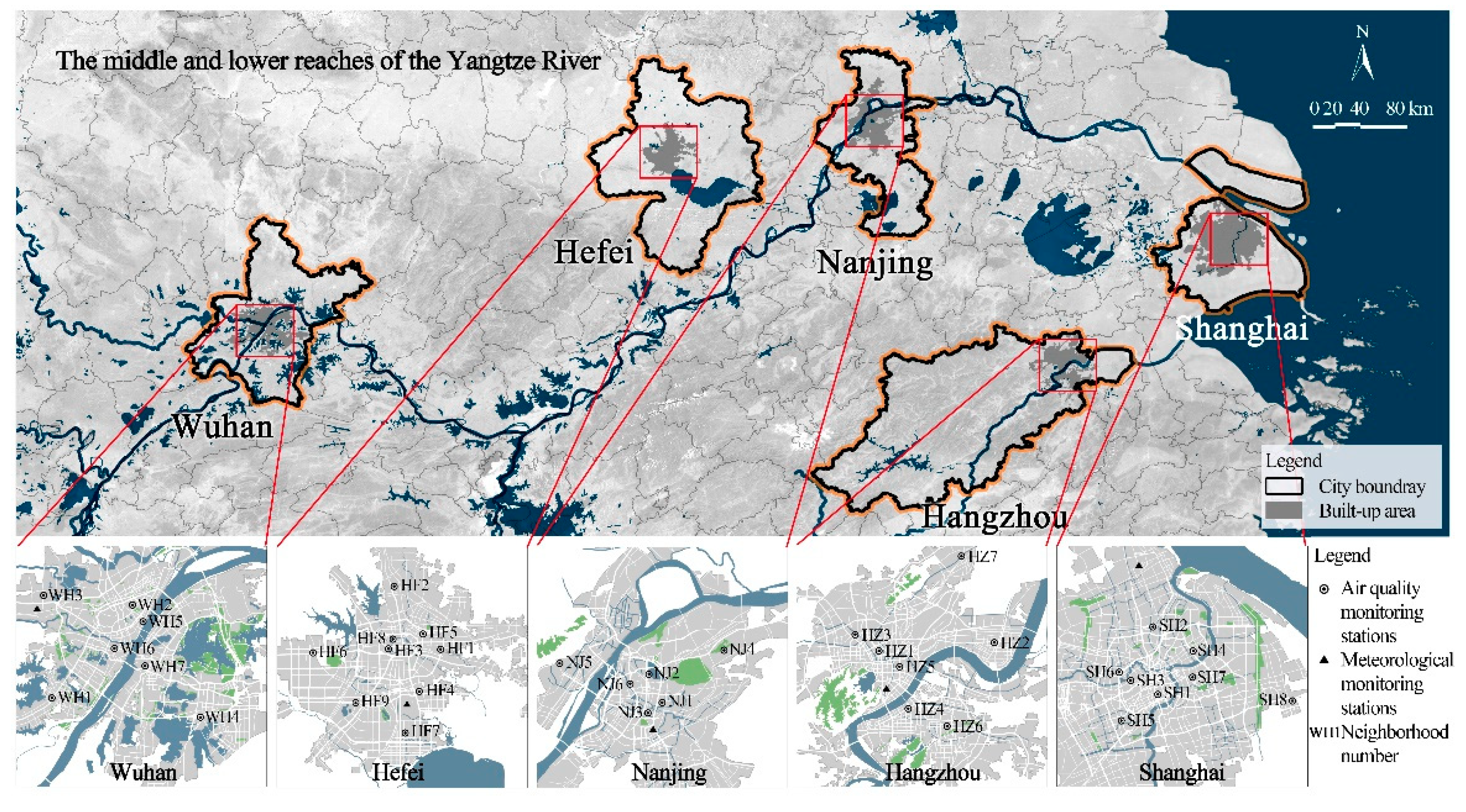
Figure 2.
The process of PM2.5 data.

Figure 3.
Variance and eigenvalue of principal factors at: (a) Overall pollution level; (b) Slight, moderate, and heavy pollution level.
Figure 3.
Variance and eigenvalue of principal factors at: (a) Overall pollution level; (b) Slight, moderate, and heavy pollution level.
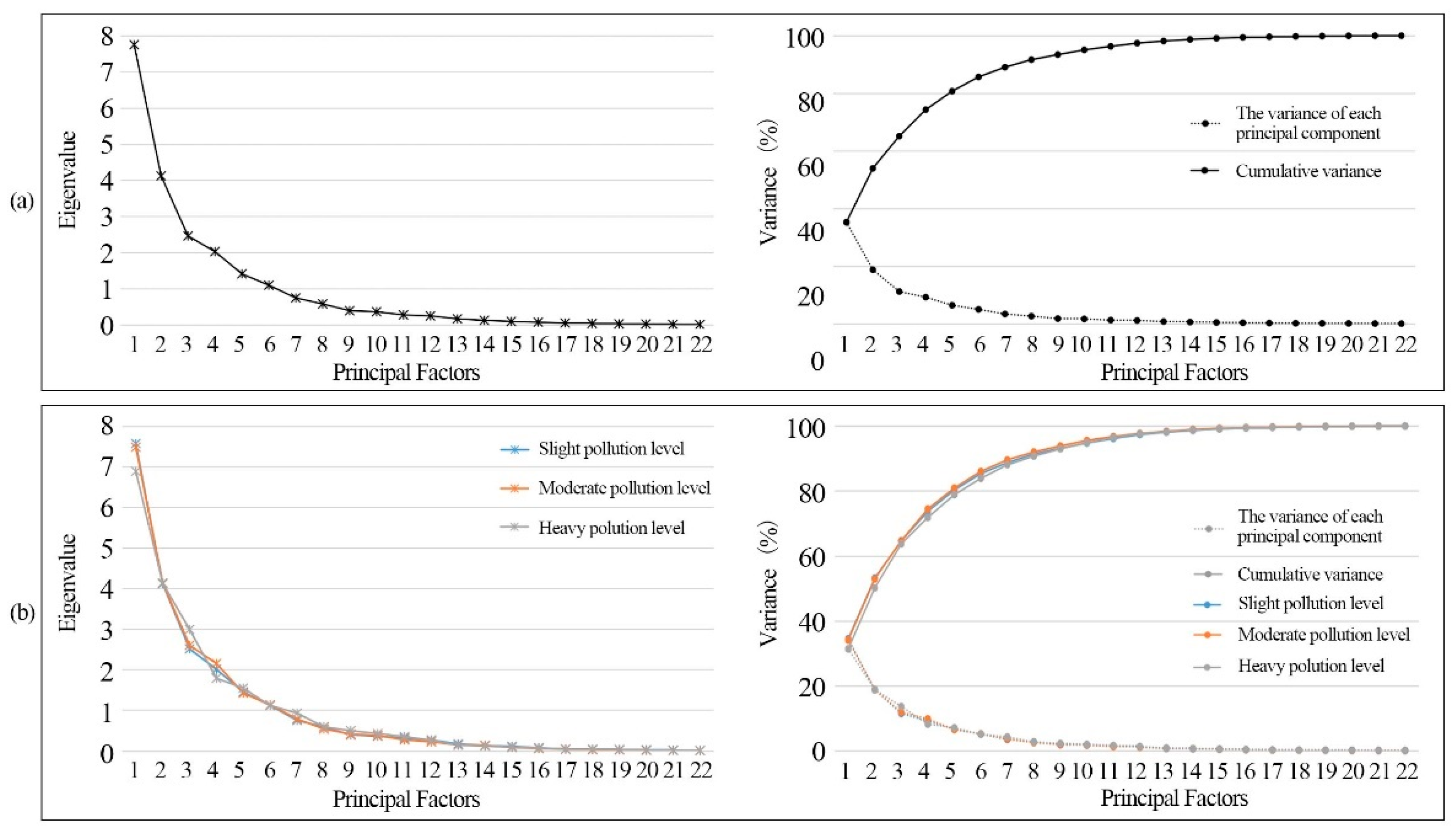
Figure 4.
Validation for regression models of six PM2.5 indicators at the different pollution levels. (a) Cin; (b) Δtin; (c) Cin’; (d) Cde; (e) Δtde; (f) Cde’.
Figure 4.
Validation for regression models of six PM2.5 indicators at the different pollution levels. (a) Cin; (b) Δtin; (c) Cin’; (d) Cde; (e) Δtde; (f) Cde’.

Figure 5.
Frequency of principal factors that significantly influence PM2.5.
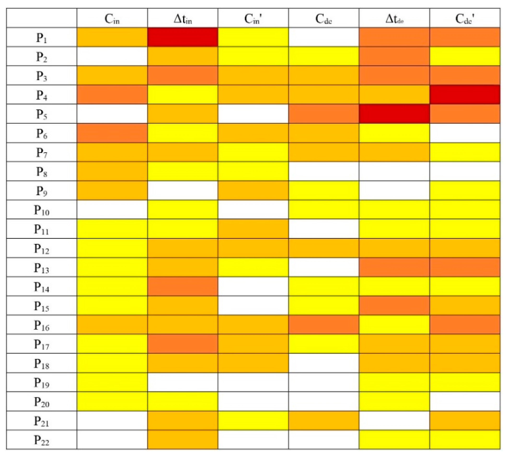
Figure 6.
Neighborhoods with (a) strong and (b) weak PM2.5 reduction capacity.


Table 1.
Indicators for model building.
| Dimension | Independent Variables | Dependent Variables | ||
|---|---|---|---|---|
| Green Space | Gray Space | Meteorological Factors | ||
| Quantity | TCR (x1), GCR (x2) | HSCR (x10) | Ta (x20), RH (x21), V (x22) | Cin (y1), Δtin (y2), Cin’ (y3), Cde (y4), Δtde (y5), Cde’ (y6) |
| Spatial Pattern | Core (x3), Islet (x4), Perforation (x5), Edge (x6), Loop (x7), Bridge (x8), Branch (x9) | BD_1 (x11), BD_2 (x12), BD_3 (x13), FAR (x14), H (x15), Hσ (x16), BEI (x17), SVF (x18), RD (x19) | ||
Table 2.
Regression model of principal factors at the overall pollution level.
| Dependent Variable | Principal Factors | Constant | p-Value | F-Value | Adj_R2 |
|---|---|---|---|---|---|
| Cin | P3(0.058,0.429) ***, P4(0.060,0.361) **, P20(−0.521,−0.340) ** | 1.424 *** | 0.002 | 6.492 | 0.347 |
| Δtin | P1(−0.037,−0.182) *, P3(0.142,0.391) ***, P4(0.089,0.199) *, P5(−0.146,−0.283) **, P7(−0.118,−0.189) *, P13(−0.367,−0.251) **, P15(0.353,0.191) *, P16(−0.586,−0.284) **, P17(0.654,0.246) **, P18 (−0.729, −0.227) **, P22 (3.749, 0.295) ** | 7.725 *** | 0.000 | 6.962 | 0.679 |
| Cin’ | P11(−0.021,−0.416) **, P16(0.027,0.298) *, P18(0.041,0.286) * | 0.199 *** | 0.015 | 4.128 | 0.232 |
| Cde | P4(−0.010,−0.354) ***, P5(0.017,0.532) ***, P12(0.020,0.287) **, P16(0.045,0.346) ***, P21(−0.118,−0.256) ** | 0.539 *** | 0.000 | 10.520 | 0.606 |
| Δtde | P1(−0.053,−0.269) ***, P2(−0.069,−0.253) ***, P3(0.079,0.222) **, P4(0.200,0.457) ***, P5(−0.154,−0.302) ***, P10(0.150,0.153) *, P13(0.430,0.299) ***, P15(0.713,0.393) ***, P17(0.788,0.301) ***, P18(0.449,0.142) *, P20(−0.692,−0.172) ** | 6.508 *** | 0.000 | 13.228 | 0.813 |
| Cde’ | P3(−0.002,−0.265) ***, P4(−0.003,−0.374) ***, P5(0.004,0.415) ***, P10(−0.004,−0.194) **, P13(−0.010,−0.327) ***, P15(−0.012,−0.326) ***, P16(0.008,0.176) *, P17(−0.021,−0.385) ***, P18(−0.017,−0.251) *** | 0.100 *** | 0.000 | 12.783 | 0.774 |
Note: ***, **, and * indicate that the factors passed the test of significance at 1%, 5%, and 10%, respectively, and the numbers in brackets indicate the regression coefficient and standardization coefficient, respectively.
Publisher’s Note: MDPI stays neutral with regard to jurisdictional claims in published maps and institutional affiliations. |
© 2022 by the authors. Licensee MDPI, Basel, Switzerland. This article is an open access article distributed under the terms and conditions of the Creative Commons Attribution (CC BY) license (https://creativecommons.org/licenses/by/4.0/).
Share and Cite
MDPI and ACS Style
Chen, M.; Dai, F. PCA-Based Identification of Built Environment Factors Reducing PM2.5 Pollution in Neighborhoods of Five Chinese Megacities. Atmosphere 2022, 13, 115. https://doi.org/10.3390/atmos13010115
AMA Style
Chen M, Dai F. PCA-Based Identification of Built Environment Factors Reducing PM2.5 Pollution in Neighborhoods of Five Chinese Megacities. Atmosphere. 2022; 13(1):115. https://doi.org/10.3390/atmos13010115
Chicago/Turabian StyleChen, Ming, and Fei Dai. 2022. "PCA-Based Identification of Built Environment Factors Reducing PM2.5 Pollution in Neighborhoods of Five Chinese Megacities" Atmosphere 13, no. 1: 115. https://doi.org/10.3390/atmos13010115
Note that from the first issue of 2016, this journal uses article numbers instead of page numbers. See further details here.