
Efficient Approaches for Solving Systems of Nonlinear Time-Fractional Partial Differential Equations


Abstract
:1. Introduction
2. Preliminaries
3. Idea of the Used Methods
3.1. Analysis of the MGMLFM
3.2. LADM for System of FDEs
4. Applications and Results
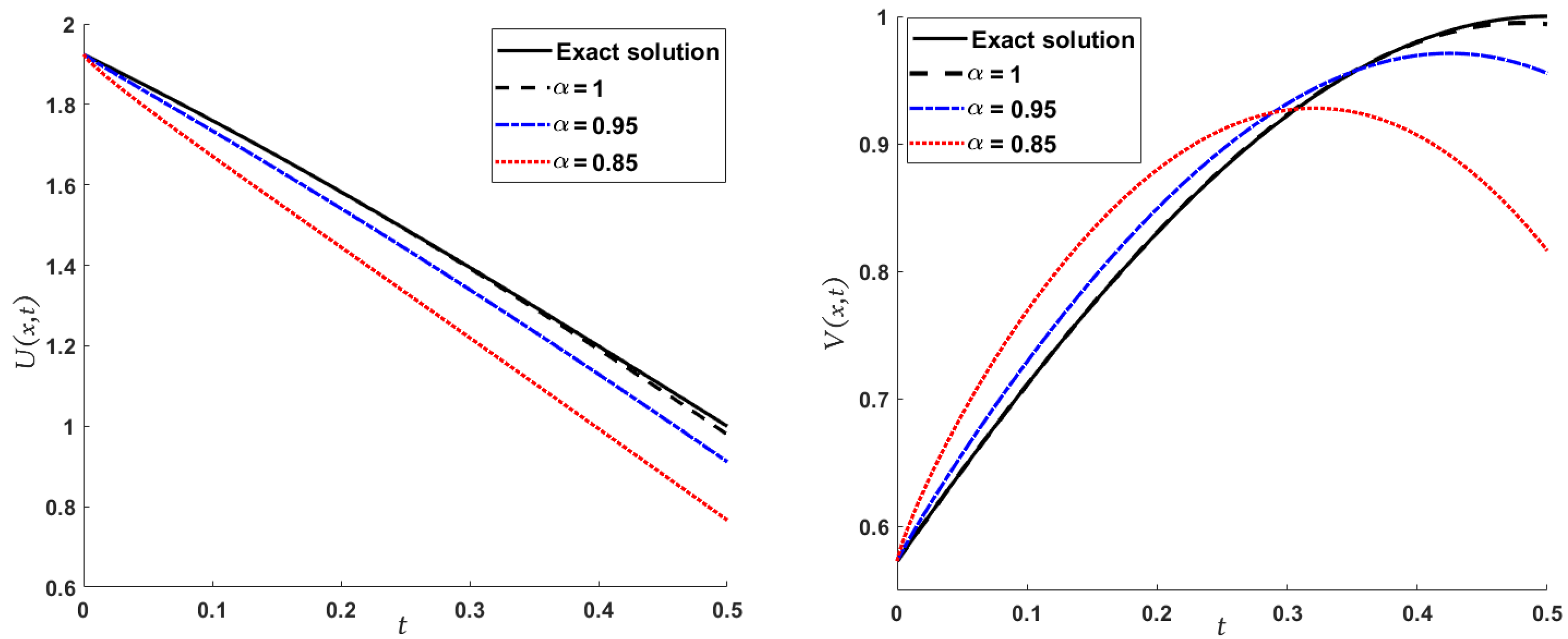
- where are coefficients. From ICs (2), we have and By using Equation (11), we write the linear term of (1) as follows:Similarly, the nonlinear term of Equation (1) is given aswhereThen, the RR are given bySubstituting the values of n and doing some computation, we obtain the following:
- To implement the LADM, we take the Laplace transform of Equation (1); then,and by using the differential property of the Laplace transform, we have:As in the LADM, the solution can be represented as an infinite seriesand the nonlinear term in Equation (1) can be decomposed aswhere and are Adomian polynomials, which can be calculated by the following formulas:By applying the inverse Laplace transform on both sides of Equation (25), we obtainwhereThe nonlinear terms and can be written as:In order to obtain the other terms of the projected solutions, we substitute the values of Equations (27) and (28) into Equation (26), yielding:Finally, we approximate the analytic solution and by
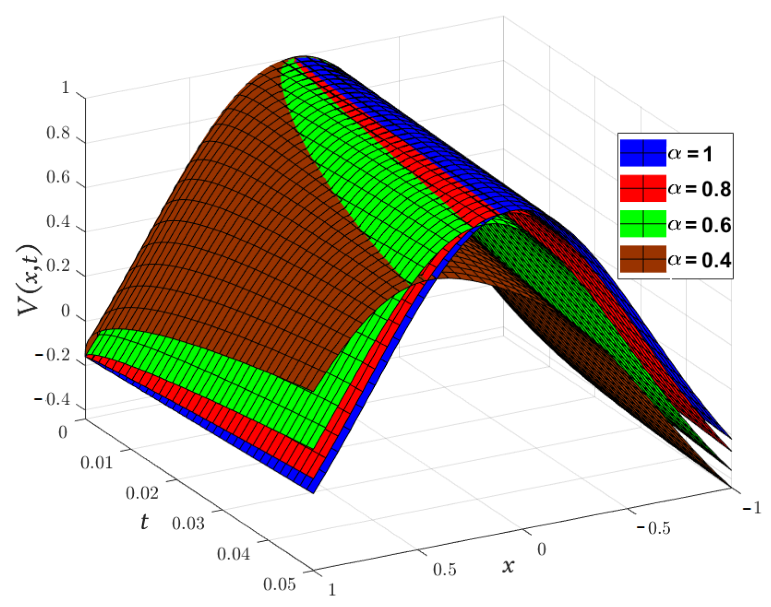
- From ICs (4), we have and By using Equation (11), we obtain the linear term of Equation (3) as follows:Similarly, the nonlinear term of Equation (3) can be written as:Then, the RR are given by:By substituting values of n, we have:
- To implement the LADM, we take the Laplace transform of both sides of Equation (3); then,using the properties of the Laplace transform, we obtain:The next step in the LADM is to represent the solution as Equation (23), and the nonlinear terms and are decomposed aswhere and are Adomian polynomials and their components are defined as:Applying the inverse Laplace transform on both sides of Equation (33), we getwhereFor the other terms, we can write:Finally, we approximate the analytic solution and by
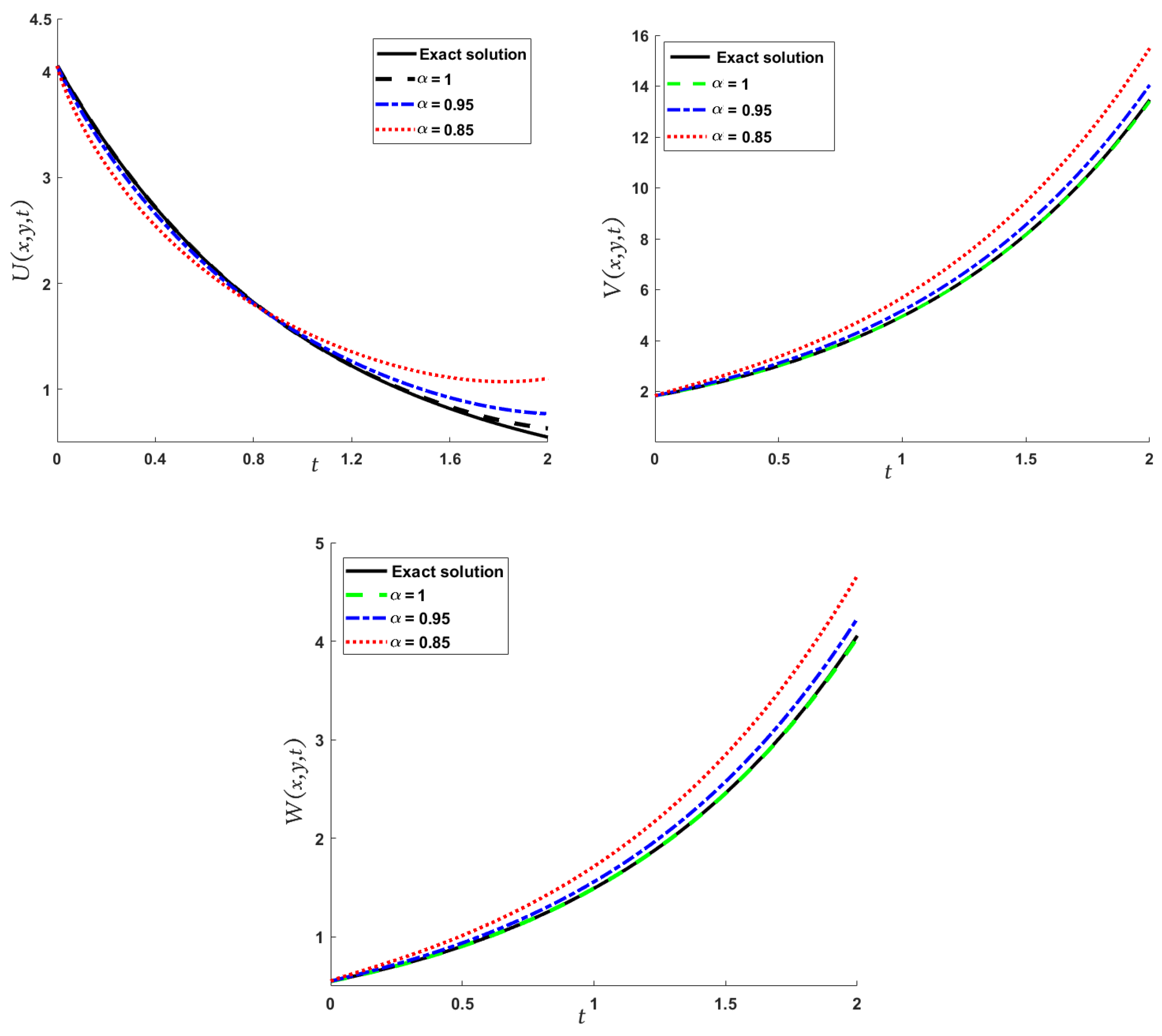
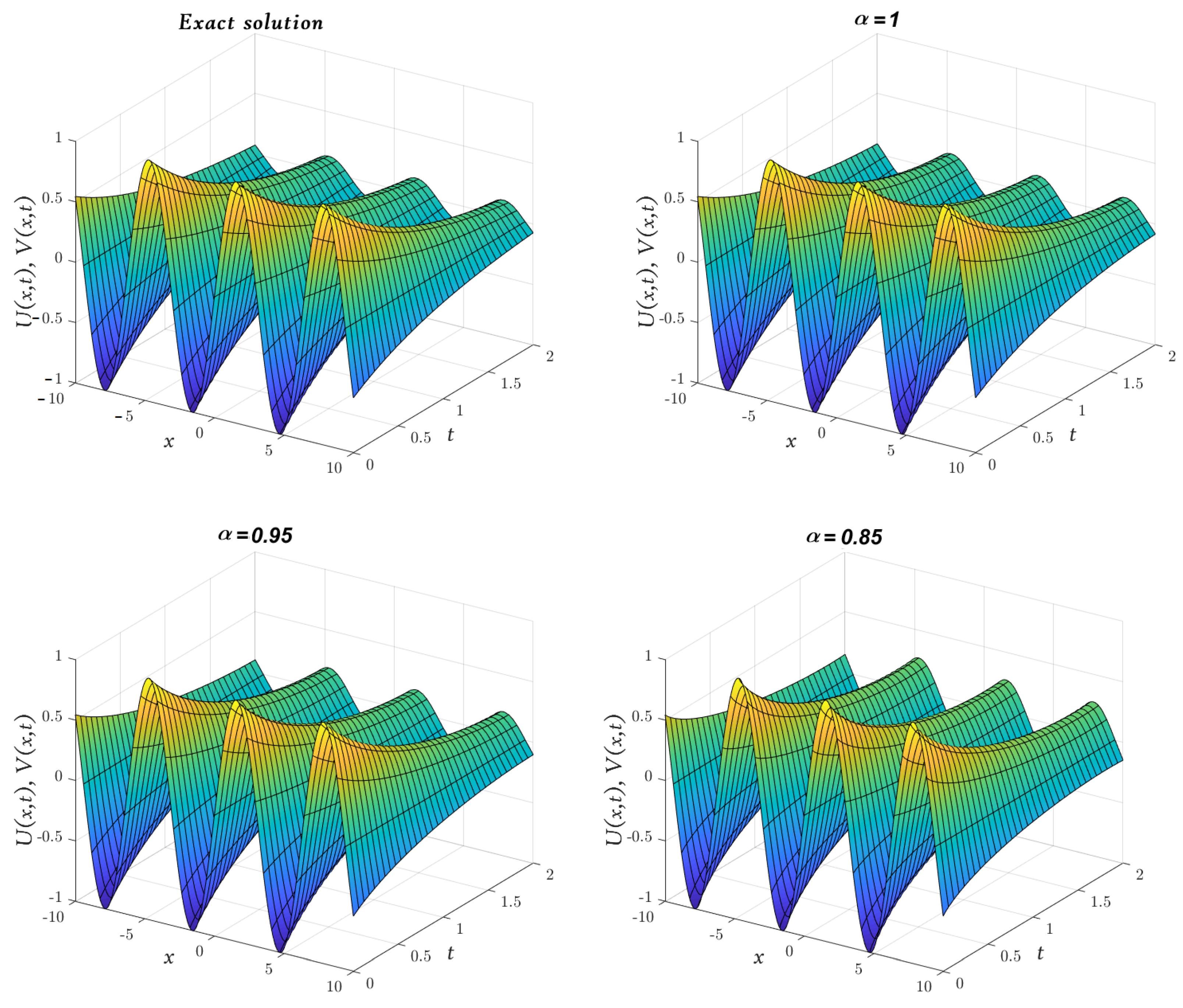
- To apply the MGMLFM, we assumewhere , and S are undetermined coefficients. From ICs (6), we have and Similarly, as in Example 2, we calculate the linear and nonlinear parts of the system (5) and using Equation (10), we getwhere and Then, the RR are given byBy substituting different values of n and using Equation (36) we get the approximate solutions in the following:
- To implement the LADM, we take the Laplace transform of Equation (5),using the Laplace transform of the Caputo derivative, we haveRepresenting the solution , and as an infinite series, as follows,the nonlinear terms included in Equation (5) can be decomposed aswhere and are Adomian polynomials defined as:by apply the inverse Laplace transform to Equation (40), we getwhereThen, it follows that for the remaining terms we obtain the solutionThe other terms of and can be computed, respectively, in the same way and according to the ADM the solution is as follows:
5. Conclusions
Author Contributions
Funding
Data Availability Statement
Acknowledgments
Conflicts of Interest
References
- Tarasov, V.E. Non-Linear Macroeconomic Models of Growth with Memory. Mathematics 2020, 8, 2078. [Google Scholar] [CrossRef]
- Sardar, T.; Rana, S.; Bhattacharya, S.; Al-Khaled, K.; Chattopadhyay, J. A generic model for a single strain mosquito-transmitted disease with memory on the host and the vector. Math. Biosci. 2015, 263, 18–36. [Google Scholar] [CrossRef] [PubMed]
- Tarasov, V.E. No nonlocality. No fractional derivative. Commun. Nonlinear Sci. Numer. Simul. 2018, 62, 157–163. [Google Scholar] [CrossRef] [Green Version]
- Ameen, I. Fractional Calculus: Numerical Methods and SIR Models. Ph.D. Thesis, University of Padova, Padova, Italy, 2017. [Google Scholar]
- Tuan, N.H.; Tri, V.V.; Baleanu, D. Analysis of the fractional corona virus pandemicvia deterministic modeling. Math. Meth. Appl. Sci. 2021, 44, 1086–1102. [Google Scholar] [CrossRef]
- Kumar, S.; Ahmadian, A.; Kumar, R.; Kumar, D.; Singh, J.; Baleanu, D.; Salimi, M. An Efficient Numerical Method for Fractional SIR Epidemic Model of Infectious Disease by Using Bernstein Wavelets. Mathematics 2020, 8, 558. [Google Scholar] [CrossRef] [Green Version]
- Baleanu, D.; Agarwal, R.P. Fractional calculus in the sky. Adv. Differ. Equ. 2021, 2021, 117. [Google Scholar] [CrossRef]
- Tarasov, V.E. Fractional vector calculus and fractional Maxwell’s equations. Ann. Phys. 2008, 323, 2756–2778. [Google Scholar] [CrossRef] [Green Version]
- West, B.J.; Turalskal, M.; Grigolini, P. Fractional calculus ties the microscopic and macroscopic scales of complex network dynamics. New J. Phys. 2015, 17, 045009. [Google Scholar] [CrossRef]
- Scalar, E.; Gorenflo, R.; Mainardi, F. Fractional calculus and continuous time finance. Physica A 2000, 284, 376–384. [Google Scholar] [CrossRef] [Green Version]
- Ameen, I.; Ali, H.M.; Alharthi, M.; Abdel-Aty, A.-H.; Elshehabey, H.M. Investigation of the dynamics of COVID-19 with a fractional mathematical model: A comparative study with actual data. Res. Phys. 2021, 23, 103976. [Google Scholar] [CrossRef]
- Ameen, I.; Sweilam, N.; Ali, H.M. A fractional-order model of human liver: Analytic-approximate and numerical solutions comparing with clinical data. Alex. Eng. J. 2021, 60, 4797–4808. [Google Scholar] [CrossRef]
- Ali, H.M.; Ameen, I. Optimal control strategies of a fractional order model for zika virus infection involving various transmissions. Chaos Solitons Fractals 2021, 146, 110864. [Google Scholar] [CrossRef]
- Ameen, I.; Baleanu, D.; Ali, H.M. An efficient algorithm for solving the fractional optimal control of SIRV epidemic model with a combination of vaccination and treatment. Chaos Solitons Fractals 2020, 137, 109892. [Google Scholar] [CrossRef]
- Hilfer, R. Applications of Fractional Calculus in Physics; World Scientific: Singapore, 2000. [Google Scholar]
- Jaradat, A.; Noorani, M.S.M.; Alquran, M.; Jaradat, H.M. A novel method for solving Caputo-time-fractional dispersive long wave Wu-Zhang system. Nonlinear Dyn. Syst. Theory 2018, 18, 182–190. [Google Scholar]
- Ali, H.M.; Pereira, F.L.; Gama, S. A new approach to the Pontryagin maximum principle for nonlinear fractional optimal control problems. Math. Meth. Appl. Sci. 2016, 39, 3640–3649. [Google Scholar] [CrossRef] [Green Version]
- Syam, M.I.; Jaradat, H.M.; Alquran, M.; Al-Shara, S. An accurate method for solving a singular second-order fractional Emden-Fowler problem. Adv. Differ. Equ. 2018, 2018, 30. [Google Scholar] [CrossRef]
- Alquran, M.; Jaradat, I. A novel scheme for solving Caputo time-fractional nonlinear equations: Theory and application. Nonlinear Dyn. 2018, 91, 2389–2395. [Google Scholar] [CrossRef]
- Dhaigude, D.B.; Birajdar, G.A. Numerical Solution of Fractional Partial Differential Equations by Discrete Adomian Decomposition Method. Adv. Appl. Math. Mech. 2014, 6, 107–119. [Google Scholar] [CrossRef]
- He, J.H. A short remark on fractional variational iteration method. Phys. Lett. A 2011, 375, 3362–3364. [Google Scholar] [CrossRef]
- AL-Saif, A.S.J.; Hattim, T.A.K. Variational iteration method for solving some models of nonlinear partial differential equations. Int. J. Pure Appl. Sci. Technol. 2011, 4, 30–40. [Google Scholar]
- Alao, S.; Oderinu, R.A.; Akinpelu, F.O.; Akinola, E.I. Homotopy analysis decomposition method for the solution of viscous boundary layer flow due to a moving sheet. J. Adv. Math. Comput. Sci. 2019, 32, 1–7. [Google Scholar] [CrossRef]
- Arafa, A.A.M.; Rida, S.Z.; Mohamed, H. Approximate analytical solutions of Schnakenberg systems by homotopy analysis method. Appl. Math. Mod. 2012, 36, 4789–4796. [Google Scholar] [CrossRef]
- Arafa, A.A.M.; Rida, S.Z.; Mohamed, H. An application of the homotopy analysis method to the transient behavior of a biochemical reaction model. Inf. Sci. Lett. 2014, 3, 29–33. [Google Scholar] [CrossRef] [Green Version]
- Arafa, A.A.M.; Rida, S.Z.; Mohamed, H. Homotopy analysis method for solving biological population model. Commun. Theor. Phys. 2011, 56, 797–800. [Google Scholar] [CrossRef]
- Javeed, S.; Baleanu, D.; Waheed, A.; Khan, M.S.; Affan, H. Analysis of homotopy perturbation method for solving fractional order differential equations. Mathematics 2019, 7, 40. [Google Scholar] [CrossRef] [Green Version]
- He, J.H. Application of homotopy perturbation method to nonlinear wave equation. Chaos Solitons Fractals 2005, 26, 695–700. [Google Scholar] [CrossRef]
- Ganji, D.D.; Sadighi, A. Application of homotopy perturbation and variational iteration methods to nonlinear heat transfer and porous media equations. J. Comput. Appl. Math. 2007, 207, 699–708. [Google Scholar] [CrossRef] [Green Version]
- Arafa, A.A.M.; Rida, S.Z.; Mohammadein, A.A.; Ali, H.M. Solving nonlinear fractional differential equation by generalized Mittag–Leffler function method. Commun. Theor. Phys. 2013, 59, 661–663. [Google Scholar] [CrossRef]
- Ali, H.M. New approximate solutions to fractional smoking model using the generalized Mittag–Leffler function method. Progr. Fract. Differ. Appl. 2019, 5, 319–326. [Google Scholar]
- Mahdy, A.M.S.; Sweilam, N.H.; Higazy, M. Approximate solution for solving nonlinear fractional order smoking model. Alex. Eng. J. 2020, 59, 739–752. [Google Scholar] [CrossRef]
- Arafa, A.A.M.; Rida, S.Z.; Ali, H.M. Generalized Mittag–Leffler function method for solving Lorenz system. Inter. J. Innov. Appl. Stud. 2013, 3, 105–111. [Google Scholar]
- Suresh, P.L.; Piriadarshani, D. Mittag–Leffler function method for solving nonlinear Riccati differential equation with fractional order. JCMCC 2020, 112, 287–296. [Google Scholar]
- Liu, Y.; Sun, H.; Yin, X.; Xin, B. A new Mittag–Leffler function undetermined coefficient method and its applications to fractional homogeneous partial differential equations. J. Nonlinear Sci. Appl. 2017, 10, 4515–4523. [Google Scholar] [CrossRef] [Green Version]
- Ali, H.M. An efficient approximate-analytical method to solve time-fractional KdV and KdVB equations. Inf. Sci. Lett. 2020, 9, 189–198. [Google Scholar]
- Ali, H.M.; Ameen, I. An efficient approach for solving fractional dynamics of a Predator-Prey system. Mod. Appl. Sci. 2019, 13, 116–126. [Google Scholar]
- Adomian, G. A review of the decomposition method in applied mathematics. Math. Anal. Appl. 1988, 135, 501–544. [Google Scholar] [CrossRef] [Green Version]
- Adomian, G.; Rach, R. Multiple decomposition for computational convenience. Appl. Math. Lett. 1990, 3, 97–99. [Google Scholar]
- Adomian, G. Solving frontier problems of physics. In The Decomposition Method, with a Preface by Yves Cherruault, Fundamental Theories of Physics; Kluwer Academic Publishers Group: Dordrecht, The Netherlands, 1994. [Google Scholar]
- Mohamed, M.Z.; Elzaki, T.M. Comparison between the Laplace Decomposition Method and Adomian Decomposition in Time-Space Fractional Nonlinear Fractional Differential Equations. Appl. Math. 2018, 9, 448–458. [Google Scholar] [CrossRef] [Green Version]
- Xu, J.; Khan, H.; Shah, R.; Alderremy, A.A.; Aly, S.; Baleanu, D. The analytical analysis of nonlinear fractional-order dynamical models. AIMS Math. 2021, 6, 6201–6219. [Google Scholar] [CrossRef]
- Haq, F.; Shah, K.; Al-Mdallal, Q.M.; Jarad, F. Application of a hybrid method for systems of fractional order partial differential equations arising in the model of the one-dimensional KellerSegel equation. Eur. Phys. J. Plus 2019, 134, 461. [Google Scholar] [CrossRef]
- Mahmood, S.; Shah, R.; Arif, M. Laplace adomian decomposition method for multi dimensional time fractional model of Navier–Stokes equation. Symmetry 2019, 11, 149. [Google Scholar] [CrossRef] [Green Version]
- Ali, A.; Humaira, L.; Shah, K. Analytical solution of general fishers equation by using Laplace Adomian decomposition method. J. Pure Appl. Math. 2018, 2, 1–4. [Google Scholar]
- Khan, H.; Shah, R.; Kumam, P.; Baleanu, D.; Arif, M. An efficient analytical technique, for the solution of fractional-order telegraph equations. Mathematics 2019, 7, 426. [Google Scholar] [CrossRef] [Green Version]
- Shah, R.; Khan, H.; Arif, M.; Kumam, P. Application of LaplaceAdomian decomposition method for the analytical solution of third-order dispersive fractional partial differential equations. Entropy 2019, 21, 335. [Google Scholar] [CrossRef] [PubMed] [Green Version]
- Rawashdeh, M. Approximate solutions for coupled systems of nonlinear PDES using the reduced differential transform method. Math. Comput. Appl. 2019, 19, 161–171. [Google Scholar] [CrossRef] [Green Version]
- Rawashdeh, M.S.; Al-Jammal, H. New approximate solutions to fractional nonlinear systems of partial differential equations using the FNDM. Adv. Differ. Equ. 2016, 2016, 235. [Google Scholar] [CrossRef] [Green Version]
- Kilbas, A.A.A.; Srivastava, H.M.; Trujillo, J.J. Theory and Applications of Fractional Differential Equations; Elsevier Science Limited: New York, NY, USA, 2006; p. 204. [Google Scholar]
- Podlubny, I. Fractional Differential Equations, Mathematics in Sciences and Engineering; Academic Press: San Diego, CA, USA, 1999. [Google Scholar]
- Miller, K.S.; Ross, B. An Introduction to the Fractional Calculus and Fractional Differential Equations; Wiley: Hoboken, NJ, USA, 1993. [Google Scholar]
- Khuri, S.A. A Laplace decomposition algorithm applied to a class of nonlinear differential equations. J. Appl. Math. 2001, 1, 141–155. [Google Scholar] [CrossRef]
- Ghorbani, A. Beyond Adomian polynomials: He polynomials. Chaos Solitons Fractals 2009, 39, 1486–1492. [Google Scholar] [CrossRef]
- Khan, H.; Shah, R.; Kumam, P.; Baleanu, D.; Arif, M. Laplace decomposition for solving nonlinear system of fractional order partial differential equations. Adv. Differ. Equ. 2020, 2020, 375. [Google Scholar] [CrossRef]
- Mohyud-Din, S.T.; Noor, M.A.; Noor, K.I. Traveling wave solutions of seventh-order generalized KdV equations using he’s polynomials. Int. J. Nonlinear Sci. Num. 2009, 10, 227–233. [Google Scholar] [CrossRef]
- Liu, Y.Q. Approximate solutions of fractional nonlinear equations using homotopy perturbation transformation method. Abstr. Appl. Anal. 2012, 2012, 752869. [Google Scholar] [CrossRef]
- Choi, J.; Kumar, D.; Singh, J.; Swroop, R. Analyttical techniques for system of time fractional nonlinear differential equations. J. Korean Math. Soci. 2017, 54, 1209–1229. [Google Scholar]


| x | t | Exact [48] | Absolute Error | |||
|---|---|---|---|---|---|---|
| MGMLFM | MGMLFM | MGMLFM | ||||
| −1 | 0.003 | −0.532386 | −0.528021 | −0.525748 | −0.525702 | 4.51907 |
| 0.006 | −0.539882 | −0.547092 | −0.528385 | −0.528205 | 1.79812 | |
| 0.009 | −0.547092 | −0.536834 | −0.531099 | −0.530696 | 4.02448 | |
| −0.5 | 0.003 | 0.0600753 | 0.0671357 | 0.0710849 | 0.0710535 | 3.13711 |
| 0.006 | 0.0489784 | 0.0598679 | 0.0664763 | 0.0663545 | 1.21755 | |
| 0.009 | 0.0392715 | 0.0531238 | 0.0619344 | 0.0616686 | 2.65732 | |
| 0.5 | 0.003 | 1.90859 | 1.91561 | 1.91955 | 1.91951 | 4.53038 |
| 0.006 | 1.8977 | 1.90838 | 1.91495 | 1.91477 | 1.80805 | |
| 0.009 | 1.88838 | 1.90171 | 1.91043 | 1.91002 | 4.05897 | |
| 1 | 0.003 | 2.51404 | 2.51836 | 2.52063 | 2.52066 | 3.28798 |
| 0.006 | 2.50673 | 2.51397 | 2.518 | 2.51813 | 1.2751 | |
| 0.009 | 2.49988 | 2.50966 | 2.5153 | 2.51558 | 2.78165 |
| x | t | Exact [48] | Absolute Error | |||
|---|---|---|---|---|---|---|
| MGMLFM | MGMLFM | MGMLFM | ||||
| −1 | 0.003 | −0.172947 | −0.167111 | −0.16387 | −0.163884 | 1.3969 |
| 0.006 | −0.182166 | −0.173109 | −0.16765 | −0.167705 | 5.5459 | |
| 0.009 | −0.190232 | −0.178702 | −0.171392 | −0.171515 | 1.23872 | |
| −0.5 | 0.003 | 0.559953 | 0.56534 | 0.56868 | 0.568529 | 1.50951 |
| 0.006 | 0.552808 | 0.559654 | 0.564751 | 0.564153 | 5.98079 | |
| 0.009 | 0.548031 | 0.554961 | 0.5611 | 0.559767 | 1.33332 | |
| 0.5 | 0.003 | 0.588096 | 0.581064 | 0.577273 | 0.577252 | 2.14755 |
| 0.006 | 0.599675 | 0.588242 | 0.581683 | 0.581597 | 8.62386 | |
| 0.009 | 0.610335 | 0.595142 | 0.586127 | 0.585932 | 1.94798 | |
| 1 | 0.003 | −0.148477 | −0.153365 | −0.156333 | −0.156208 | 1.25863 |
| 0.006 | −0.141644 | −0.148238 | −0.152846 | −0.152353 | 4.93352 | |
| 0.009 | −0.136498 | −0.143877 | −0.149575 | −0.148487 | 1.08802 |
| x | t | Exact | Absolute Error | ||||||
|---|---|---|---|---|---|---|---|---|---|
| FNDM [49] | MGMLFM | FNDM [49] | MGMLFM | FNDM [49] | MGMLFM | ||||
| −10 | 0.2 | 0.403596 | 0.3985421 | 0.429046 | 0.4274714 | 0.446097 | 0.4454068 | 0.445407 | 1.3478525 |
| 0.4 | 0.349827 | 0.3275878 | 0.358413 | 0.3487726 | 0.369934 | 0.3646684 | 0.364668 | 1.6838537 | |
| −5 | 0.2 | 0.711403 | 0.7024943 | 0.756262 | 0.7534867 | 0.786318 | 0.7851008 | 0.785101 | 2.3758057 |
| 0.4 | 0.616625 | 0.5774259 | 0.63176 | 0.6147676 | 0.652069 | 0.6427865 | 0.642786 | 2.9680616 | |
| 5 | 0.2 | −0.711403 | −0.7024943 | −0.756262 | −0.7534867 | −0.786318 | −0.7851008 | −0.785101 | 2.3758057 |
| 0.4 | −0.616625 | −0.5774259 | −0.63176 | −0.6147676 | −0.652069 | −0.6427865 | −0.642786 | 2.9680616 | |
| 10 | 0.2 | −0.403596 | −0.3985421 | −0.429046 | −0.4274714 | −0.446097 | −0.4454068 | −0.445407 | 1.3478525 |
| 0.4 | −0.349827 | −0.3275878 | −0.358413 | −0.3487726 | −0.369934 | −0.3646684 | −0.364668 | 1.6838537 | |
| x | t | Exact | Absolute Error | ||||||
|---|---|---|---|---|---|---|---|---|---|
| FNDM [49] | MGMLFM | FNDM [49] | MGMLFM | FNDM [49] | MGMLFM | ||||
| 0.5 | 0.3 | 1.6256 | 1.6241897 | 1.74178 | 1.74158 | 1.82217 | 1.8221189 | 1.82212 | 1.0285638 |
| 0.6 | 1.27791 | 1.2607914 | 1.31047 | 1.3063996 | 1.35131 | 1.3498715 | 1.34986 | 1.27012 | |
| 0.9 | 1.10414 | 1.033497 | 1.02931 | 1.0058445 | 1.0105 | 1.00021 | 1 | 2.09565 | |
| 1 | 0.3 | 2.68017 | 2.6778362 | 2.8717 | 2.871385 | 3.00424 | 3.0041662 | 3.00417 | 1.695815 |
| 0.6 | 2.10692 | 2.0786935 | 2.1606 | 2.1538889 | 2.22793 | 2.225562 | 2.22554 | 2.09407 | |
| 0.9 | 1.82042 | 1.7039486 | 1.69705 | 1.6583572 | 1.66603 | 1.649067 | 1.64872 | 3.45514 | |
| 1.5 | 0.3 | 4.41885 | 4.4150055 | 4.73464 | 4.7341143 | 4.95316 | 4.9530327 | 4.95303 | 2.7959262 |
| 0.6 | 3.47372 | 3.4271863 | 3.56223 | 3.5511624 | 3.6323 | 3.6693312 | 3.6693 | 3.45253 | |
| 0.9 | 3.00136 | 2.809336 | 2.79796 | 2.7341689 | 2.74682 | 2.718851 | 2.71828 | 5.69657 | |
| x | t | Exact | Absolute Error | ||||||
|---|---|---|---|---|---|---|---|---|---|
| FNDM [49] | MGMLFM | FNDM [49] | MGMLFM | FNDM [49] | MGMLFM | ||||
| 0.5 | 0.3 | 1.76307 | 1.7638956 | 1.58084 | 1.5809426 | 1.4918 | 1.4918246 | 1.49182 | 4.9816688 |
| 0.6 | 2.48848 | 2.5004130 | 2.17346 | 2.1758721 | 2.01296 | 2.0137461 | 2.01375 | 6.6314571 | |
| 0.9 | 3.40244 | 3.4604711 | 2.95156 | 2.9672968 | 2.71191 | 2.7181639 | 2.71828 | 1.17976 | |
| 1 | 0.3 | 2.90682 | 2.9081722 | 2.60637 | 2.6065337 | 2.45956 | 2.4596030 | 2.4596 | 8.2133832 |
| 0.6 | 4.10281 | 4.1224841 | 3.58343 | 3.5874066 | 3.31881 | 3.3201059 | 3.32012 | 1.0933424 | |
| 0.9 | 5.60968 | 5.7053523 | 4.86629 | 4.8922453 | 4.47118 | 4.4814946 | 4.48169 | 1.9450873 | |
| 1.5 | 0.3 | 4.79253 | 4.7947653 | 4.29717 | 4.2974475 | 4.05514 | 4.0551998 | 4.0552 | 1.3541579 |
| 0.6 | 6.76439 | 6.7968273 | 5.90808 | 5.9146336 | 5.47179 | 5.4739294 | 5.47395 | 1.8026169 | |
| 0.9 | 9.2488 | 9.4065356 | 8.02316 | 8.0659489 | 7.37174 | 7.3887354 | 7.38906 | 3.2069069 | |
| x | t | Exact | Absolute Error | ||||||
|---|---|---|---|---|---|---|---|---|---|
| FNDM [49] | MGMLFM | FNDM [49] | MGMLFM | FNDM [49] | MGMLFM | ||||
| 0.5 | 0.3 | 1.44348 | 1.4441556 | 1.29428 | 1.2943663 | 1.22138 | 1.2214027 | 1.2214 | 4.0786454 |
| 0.6 | 2.0374 | 2.0471650 | 1.77948 | 1.7814534 | 1.64807 | 1.6487158 | 1.64872 | 5.4293779 | |
| 0.9 | 2.78569 | 2.8331941 | 2.41653 | 2.4294171 | 2.22032 | 2.2254443 | 2.22554 | 9.65902 | |
| 1 | 0.3 | 0.875516 | 0.8759246 | 0.785023 | 0.7850729 | 0.740807 | 0.7408182 | 0.740818 | 2.4738235 |
| 0.6 | 1.23574 | 1.2416684 | 1.07931 | 1.0805061 | 0.999606 | 0.9999967 | 1 | 3.2930841 | |
| 0.9 | 1.6896 | 1.7184191 | 1.4657 | 1.4735159 | 1.34669 | 1.3498002 | 1.34986 | 5.8584905 | |
| 1.5 | 0.3 | 0.531027 | 0.5312751 | 0.47614 | 0.4761708 | 0.449322 | 0.4493289 | 0.449329 | 1.5004498 |
| 0.6 | 0.749516 | 0.7531099 | 0.654634 | 0.6553601 | 0.606291 | 0.6065287 | 0.606531 | 1.9973565 | |
| 0.9 | 1.0248 | 1.0422739 | 0.888992 | 0.8937326 | 0.816812 | 0.8186952 | 0.818731 | 3.5533541 | |
Publisher’s Note: MDPI stays neutral with regard to jurisdictional claims in published maps and institutional affiliations. |
© 2022 by the authors. Licensee MDPI, Basel, Switzerland. This article is an open access article distributed under the terms and conditions of the Creative Commons Attribution (CC BY) license (https://creativecommons.org/licenses/by/4.0/).
Share and Cite
Ali, H.M.; Ahmad, H.; Askar, S.; Ameen, I.G. Efficient Approaches for Solving Systems of Nonlinear Time-Fractional Partial Differential Equations. Fractal Fract. 2022, 6, 32. https://doi.org/10.3390/fractalfract6010032
Ali HM, Ahmad H, Askar S, Ameen IG. Efficient Approaches for Solving Systems of Nonlinear Time-Fractional Partial Differential Equations. Fractal and Fractional. 2022; 6(1):32. https://doi.org/10.3390/fractalfract6010032
Chicago/Turabian StyleAli, Hegagi Mohamed, Hijaz Ahmad, Sameh Askar, and Ismail Gad Ameen. 2022. "Efficient Approaches for Solving Systems of Nonlinear Time-Fractional Partial Differential Equations" Fractal and Fractional 6, no. 1: 32. https://doi.org/10.3390/fractalfract6010032
APA StyleAli, H. M., Ahmad, H., Askar, S., & Ameen, I. G. (2022). Efficient Approaches for Solving Systems of Nonlinear Time-Fractional Partial Differential Equations. Fractal and Fractional, 6(1), 32. https://doi.org/10.3390/fractalfract6010032