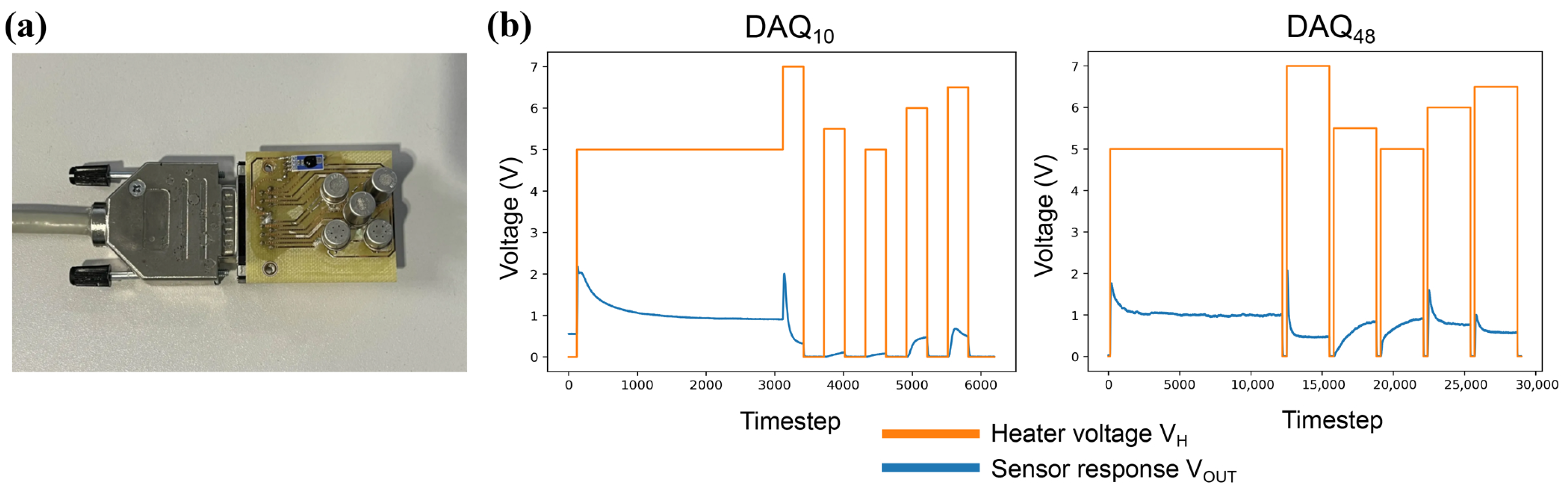
Figure 1.
(a) The sensor board used for the data acquisition. (b) Temperature modulation patterns and .
Figure 1.
(a) The sensor board used for the data acquisition. (b) Temperature modulation patterns and .
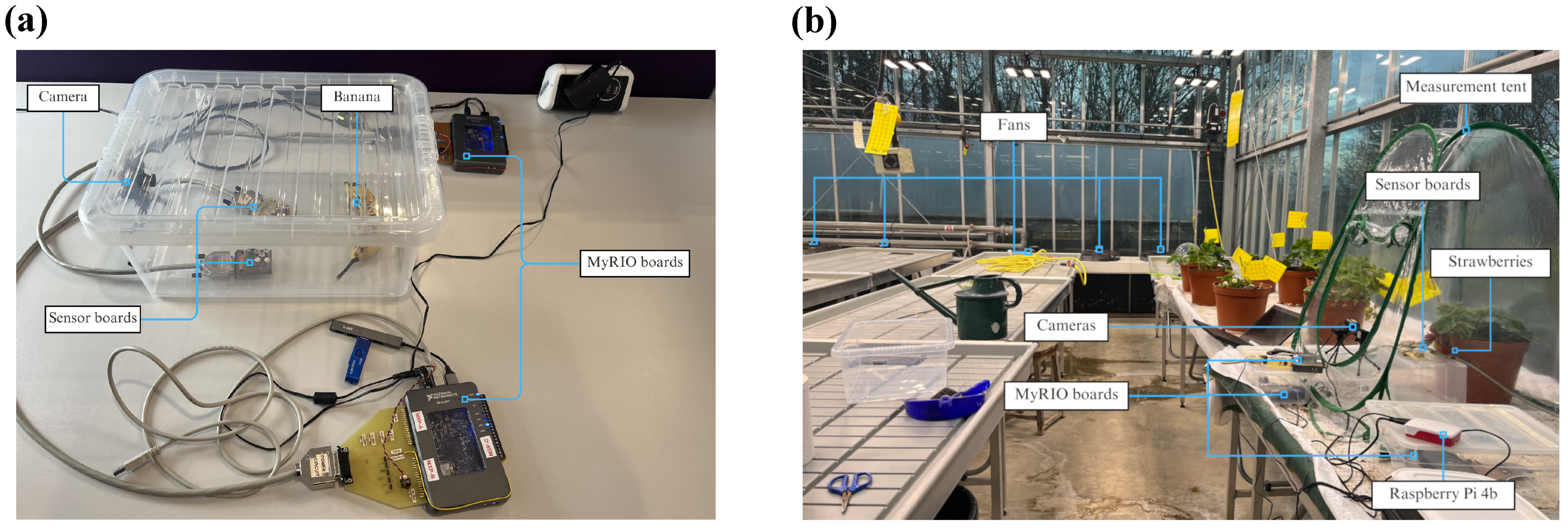
Figure 2.
The set-up for the data collection case-studies. (a) Case study 1: observing banana ripening. (b) Case-study 2: strawberry ripening inside a glasshouse.
Figure 2.
The set-up for the data collection case-studies. (a) Case study 1: observing banana ripening. (b) Case-study 2: strawberry ripening inside a glasshouse.
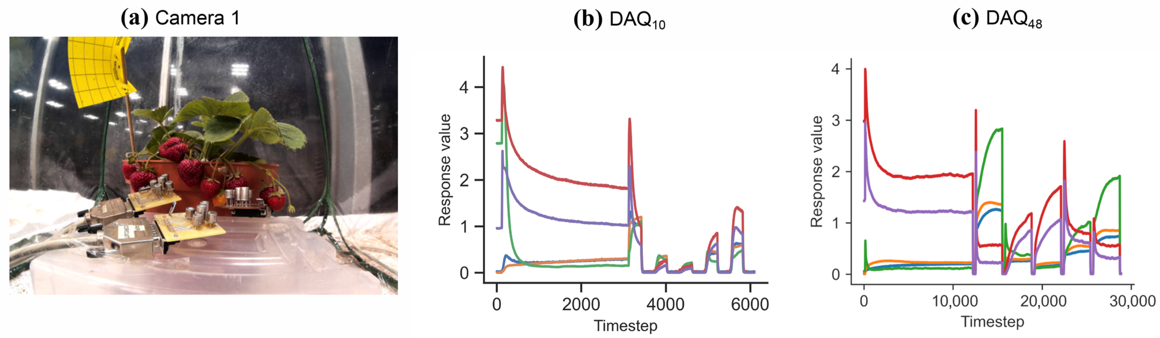
Figure 3.
Example data taken from strawberry dataset. (a) An example image from the See3CAM_CU30 camera. (b) An odour data sample acquired with . (c) An odour data sample acquired with .
Figure 3.
Example data taken from strawberry dataset. (a) An example image from the See3CAM_CU30 camera. (b) An odour data sample acquired with . (c) An odour data sample acquired with .
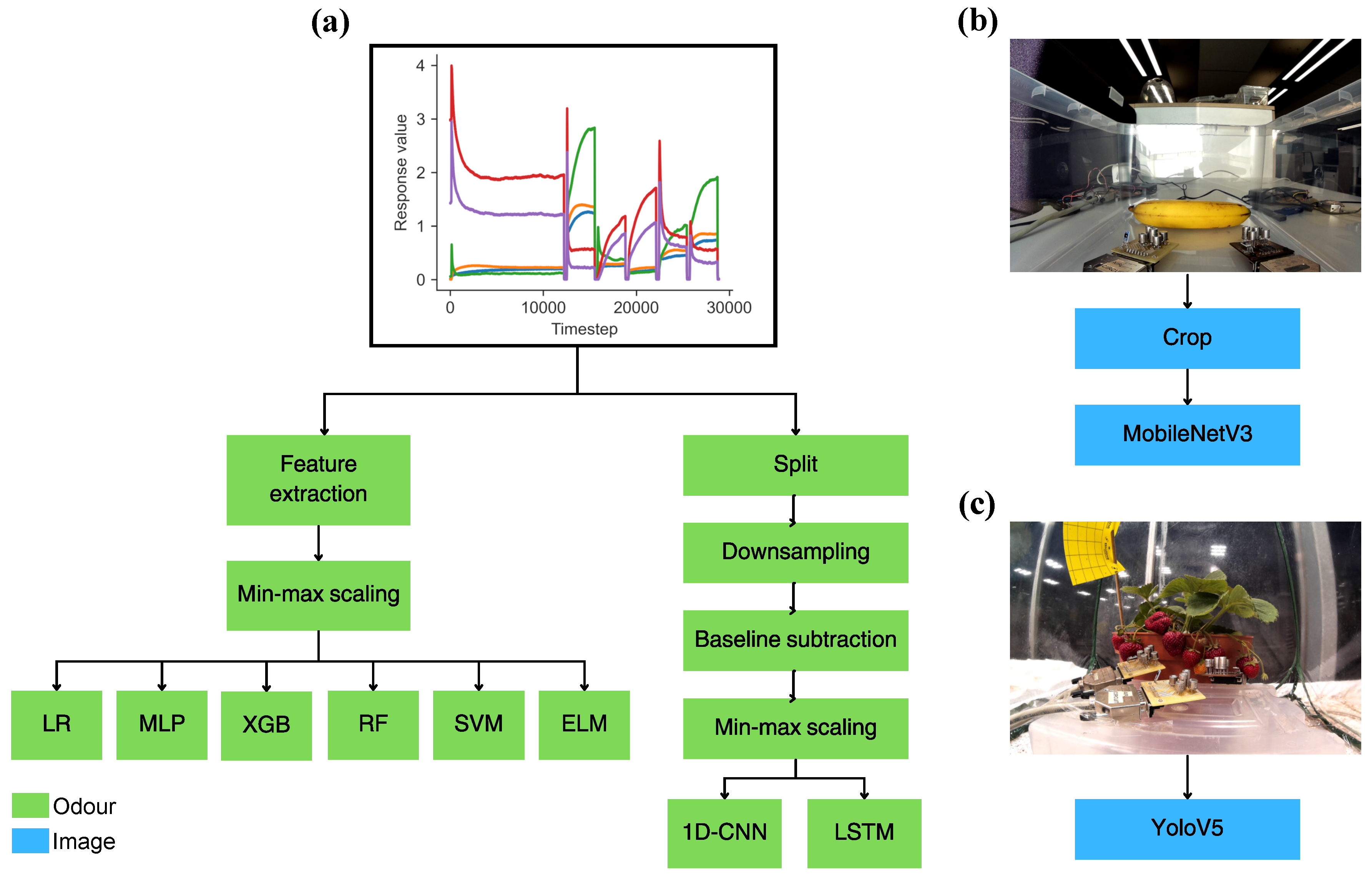
Figure 4.
The pre-processing steps and ML methods applied on the data. (a) Odour modality (both banana and strawberry data). (b) Image modality (banana data). (c) Image modality (strawberry data).
Figure 4.
The pre-processing steps and ML methods applied on the data. (a) Odour modality (both banana and strawberry data). (b) Image modality (banana data). (c) Image modality (strawberry data).
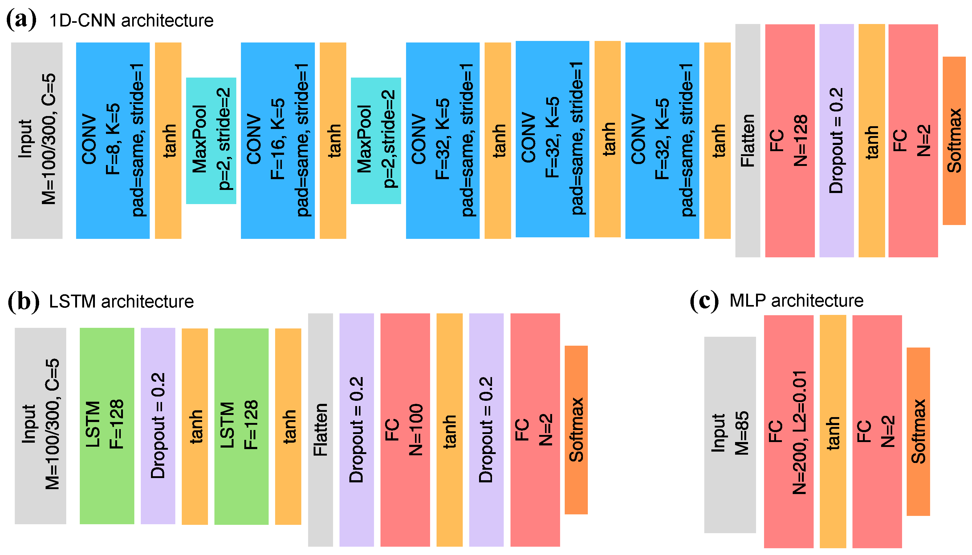
Figure 5.
The neural network architectures used for processing the odour modality. (
a) 1D-CNN architecture, based on [
55]. (
b) The stacked LSTM architecture. (
c) The 3-layer MLP architecture.
Figure 5.
The neural network architectures used for processing the odour modality. (
a) 1D-CNN architecture, based on [
55]. (
b) The stacked LSTM architecture. (
c) The 3-layer MLP architecture.
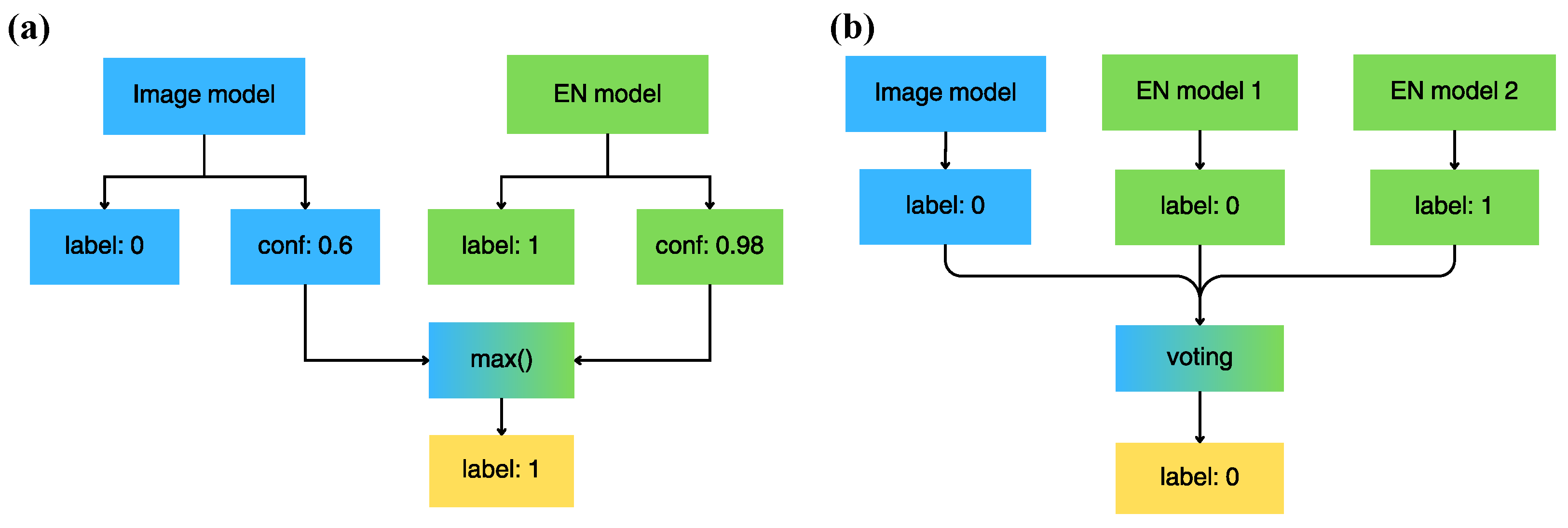
Figure 6.
Two late fusion strategies were adopted. (a) Maximum confidence fusion. (b) Majority voting.
Figure 6.
Two late fusion strategies were adopted. (a) Maximum confidence fusion. (b) Majority voting.
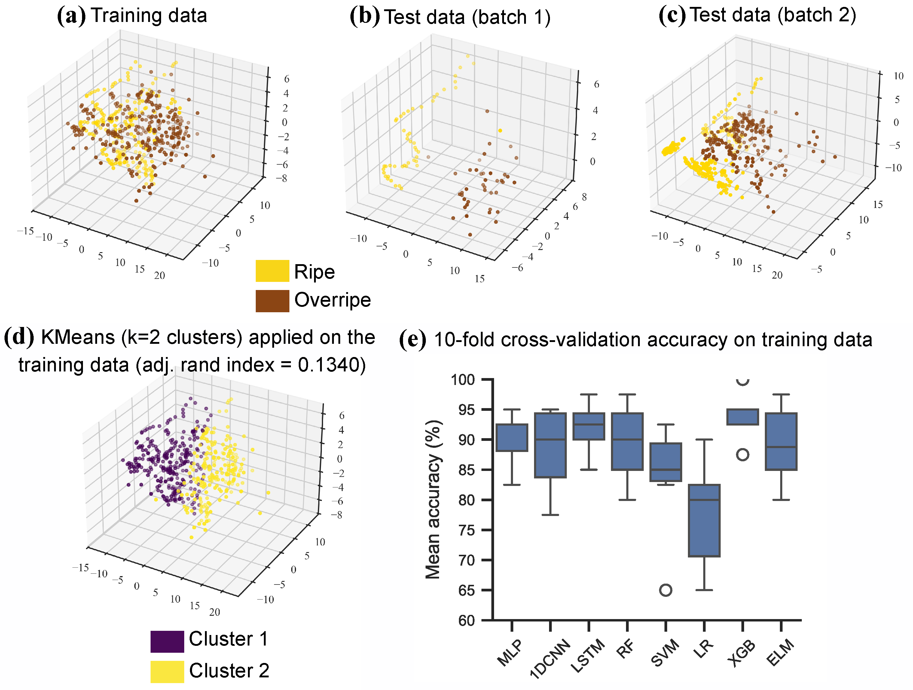
Figure 7.
Visualisation of data from in the open-air banana case study and visualisation of results of the ML models. (a–c) PCA plots of the training and test datasets. (d) KMeans (k = 2 clusters) applied on the PCA transformed training dataset. (e) Box-plot of the 10-fold cross-validation accuracy results of the ML models on the training dataset.
Figure 7.
Visualisation of data from in the open-air banana case study and visualisation of results of the ML models. (a–c) PCA plots of the training and test datasets. (d) KMeans (k = 2 clusters) applied on the PCA transformed training dataset. (e) Box-plot of the 10-fold cross-validation accuracy results of the ML models on the training dataset.
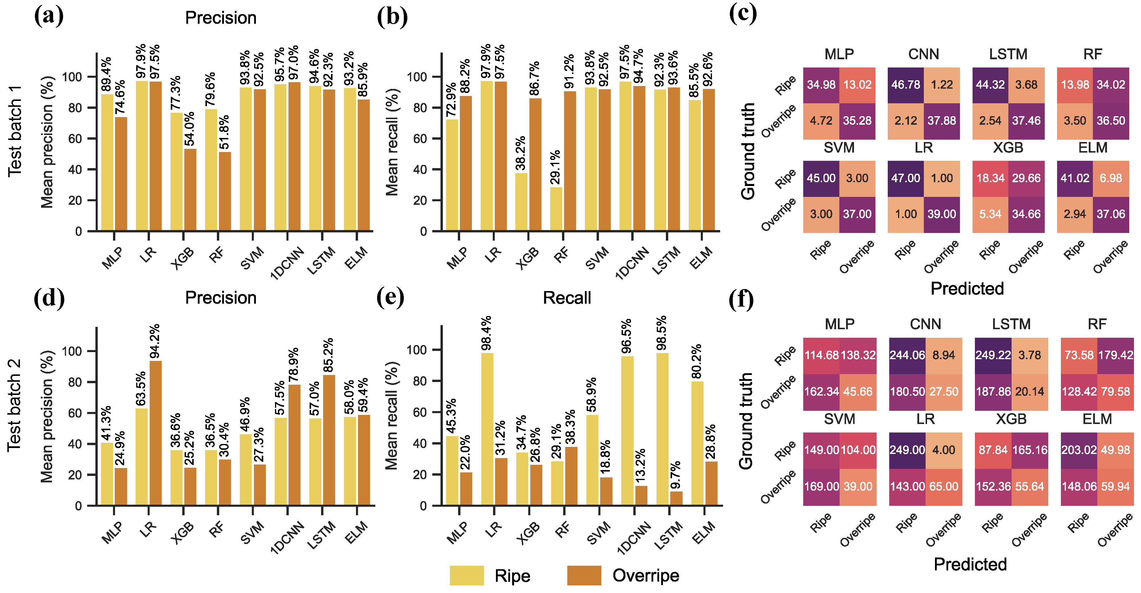
Figure 8.
Visualisation of the class-wise ML results on the banana case-study data from . All results are reported as the mean over 50 runs. (a–c) Class-wise precision and recall plots, and confusion matrices for test data batch 1. (d–f) Class-wise precision and recall plots, and confusion matrices for test data batch 2.
Figure 8.
Visualisation of the class-wise ML results on the banana case-study data from . All results are reported as the mean over 50 runs. (a–c) Class-wise precision and recall plots, and confusion matrices for test data batch 1. (d–f) Class-wise precision and recall plots, and confusion matrices for test data batch 2.
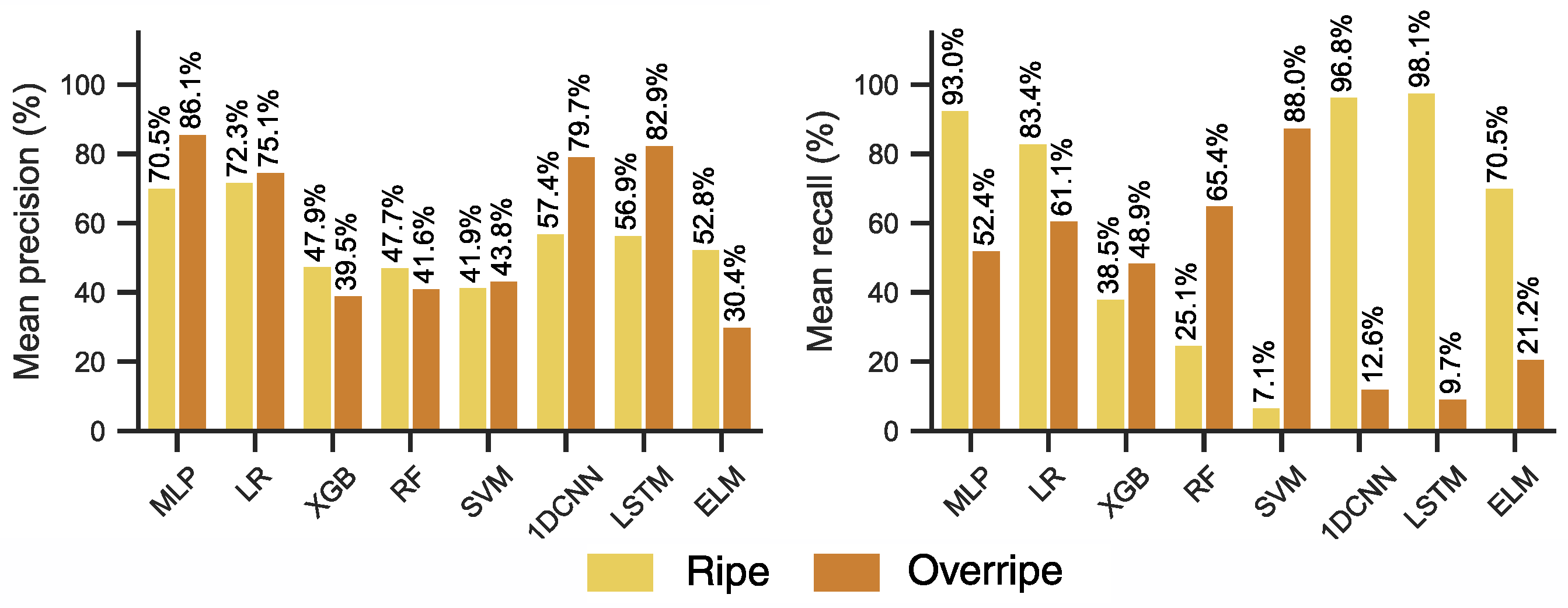
Figure 9.
Precision and recall visualised for the open-air banana ripening test data (batch 2) when models were trained on the small feature-set. Results are reported as the mean over 50 runs.
Figure 9.
Precision and recall visualised for the open-air banana ripening test data (batch 2) when models were trained on the small feature-set. Results are reported as the mean over 50 runs.
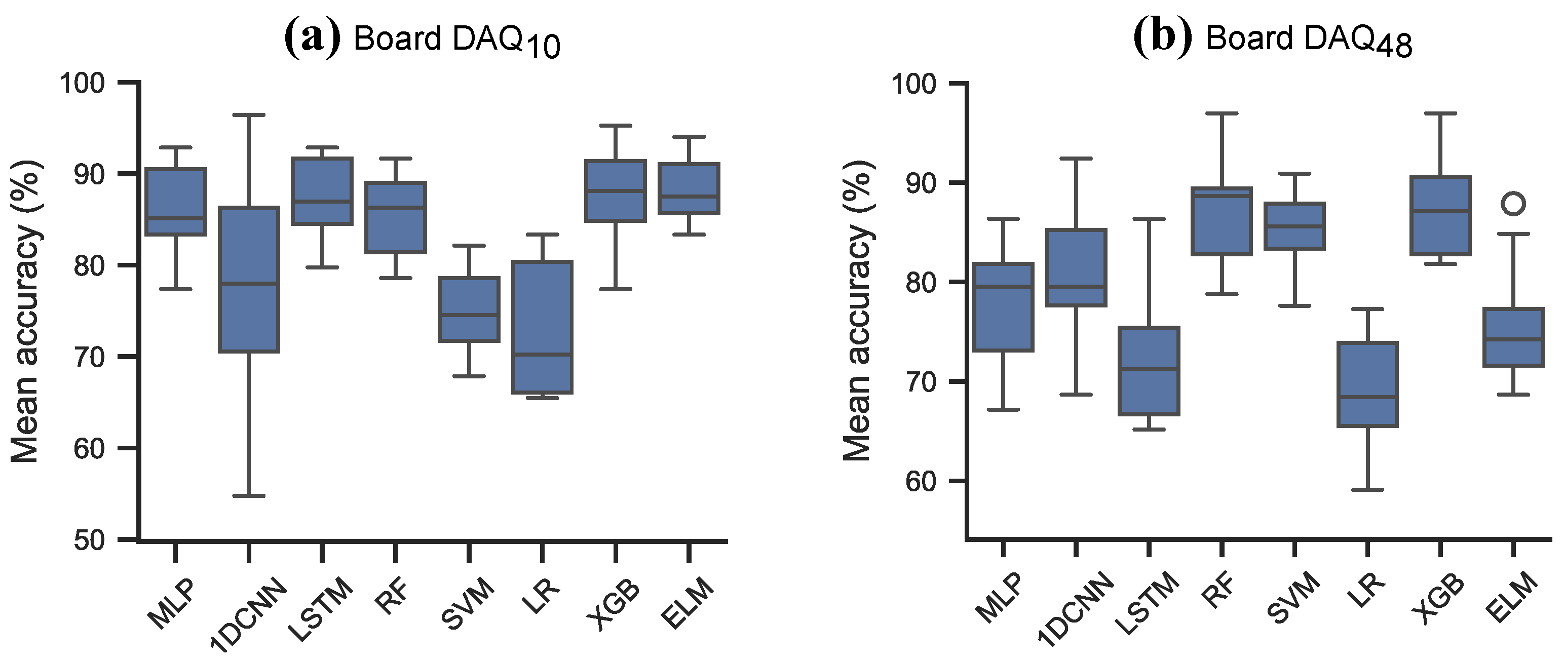
Figure 10.
10-fold cross-validation scores on the strawberry odour datasets. (a) Data from . (b) Data from .
Figure 10.
10-fold cross-validation scores on the strawberry odour datasets. (a) Data from . (b) Data from .
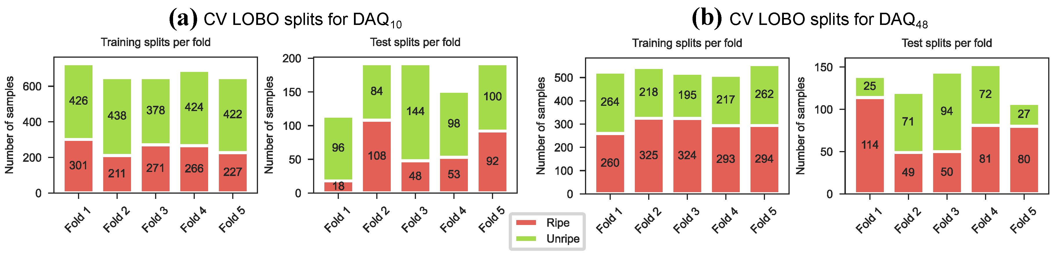
Figure 11.
Split of training and test data in the LOBO cross-validation. (a) Data from . (b) Data from .
Figure 11.
Split of training and test data in the LOBO cross-validation. (a) Data from . (b) Data from .
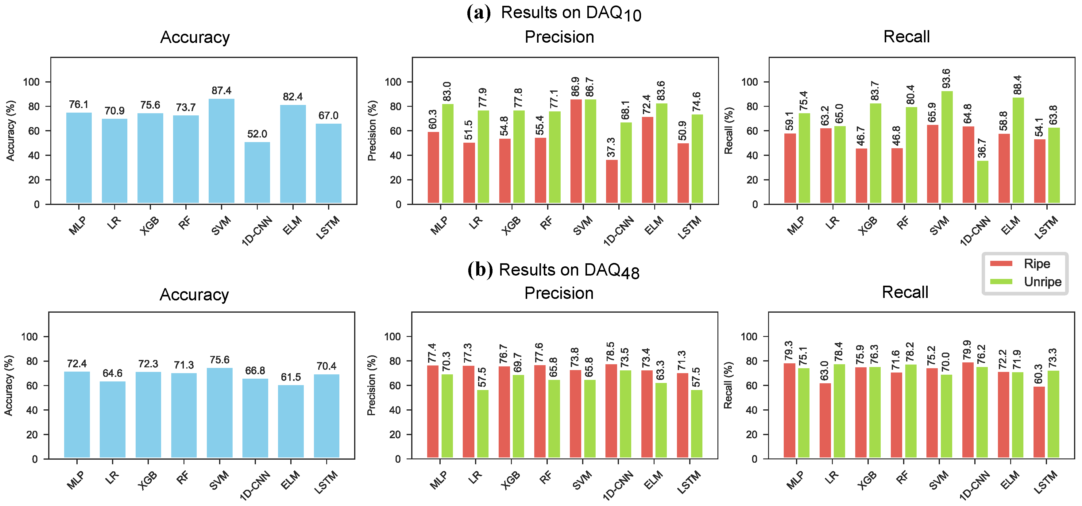
Figure 12.
Results on the strawberry data following a leave-5-day-out cross-validation strategy, averaged over 10 runs for each fold. (a) Results on . (b) Results on .
Figure 12.
Results on the strawberry data following a leave-5-day-out cross-validation strategy, averaged over 10 runs for each fold. (a) Results on . (b) Results on .
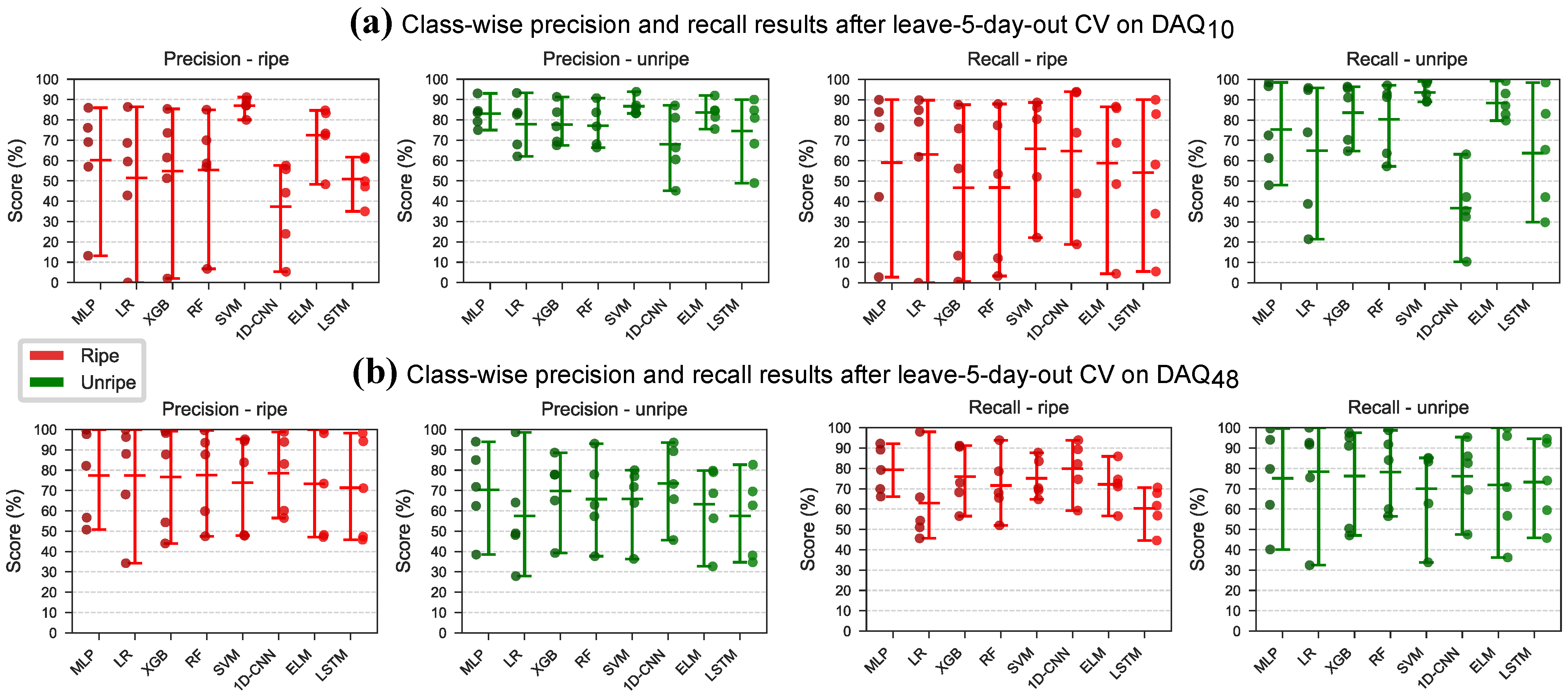
Figure 13.
The spread of the class-wise precision and recall when evaluating on the strawberry dataset with the leave-5-day-out cross-validation strategy. (a) Results on . (b) Results on .
Figure 13.
The spread of the class-wise precision and recall when evaluating on the strawberry dataset with the leave-5-day-out cross-validation strategy. (a) Results on . (b) Results on .
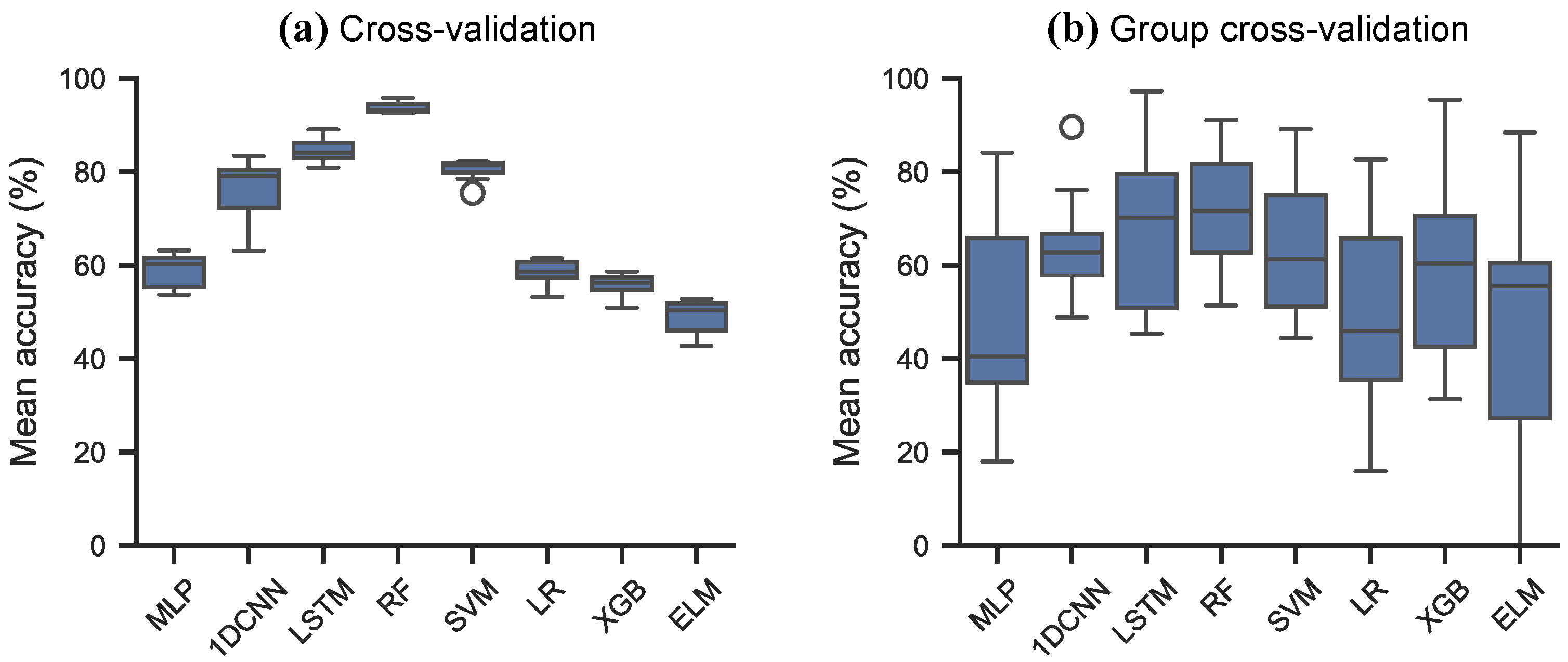
Figure 14.
Cross-validation scores on the strawberry odour dataset. (a) Stratified 10-fold cross-validation. (b) Stratified 10-fold group cross-validation.
Figure 14.
Cross-validation scores on the strawberry odour dataset. (a) Stratified 10-fold cross-validation. (b) Stratified 10-fold group cross-validation.
Figure 15.
Illustrative images of the banana images, taken from the training dataset. (a,b) Example image of a ripe banana. (c) Example image of an overripe banana. (d) Image taken at night.
Figure 15.
Illustrative images of the banana images, taken from the training dataset. (a,b) Example image of a ripe banana. (c) Example image of an overripe banana. (d) Image taken at night.
Figure 16.
Illustrative images from the strawberry image data. (a) Well-lit image of ripe strawberries, taken with Camera 1. (b) Strongly backlit images of ripe strawberries, taken with Camera 1. (c) Well-lit image of ripe strawberries, taken with Camera 2. (d) Strongly backlit images of ripe strawberries, taken with Camera 2.
Figure 16.
Illustrative images from the strawberry image data. (a) Well-lit image of ripe strawberries, taken with Camera 1. (b) Strongly backlit images of ripe strawberries, taken with Camera 1. (c) Well-lit image of ripe strawberries, taken with Camera 2. (d) Strongly backlit images of ripe strawberries, taken with Camera 2.
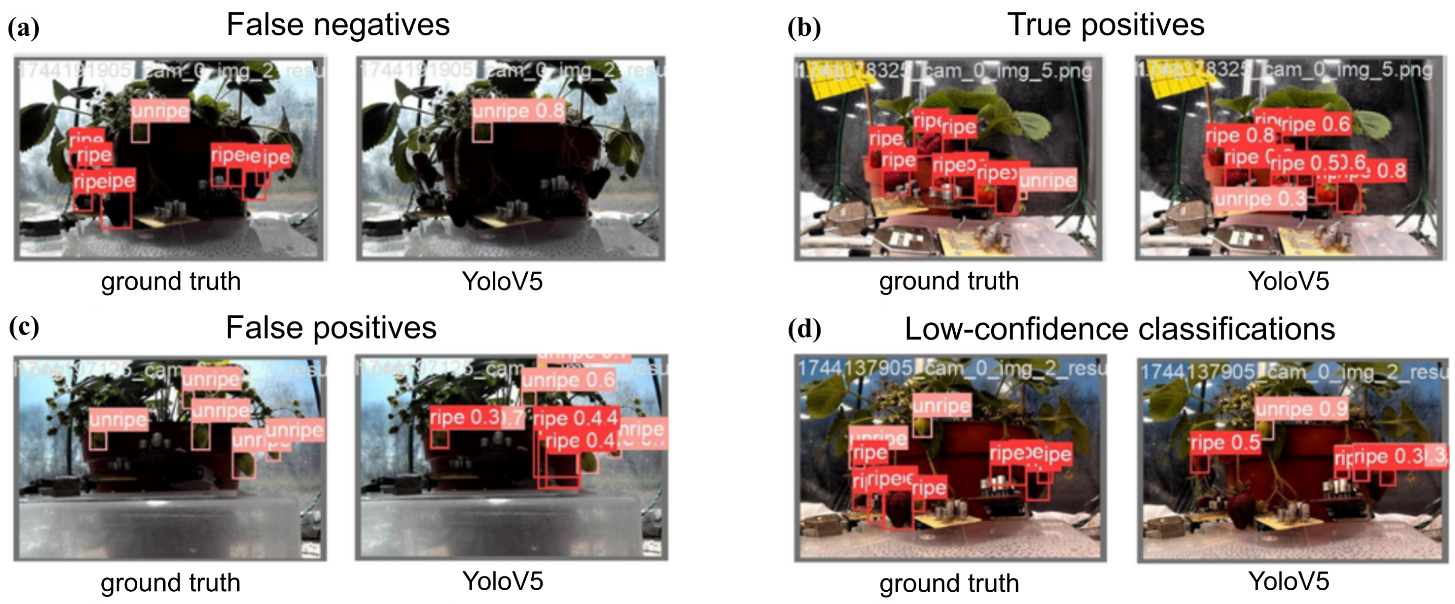
Figure 17.
Examples of annotated ground-truth and YoloV5 prediction pairs on images from camera 1. (a) On images with strong backlight, Yolov5 has poor recall, resulting in many false negatives. (b) On well-lit images, YoloV5 performed well. (c) Under strong backlight, YoloV5 often produced false positives, confusing dark foreground for ripe strawberries. (d) Although under artificial light YoloV5 performed better than on daylight images, many bounding boxes were of low-confidence.
Figure 17.
Examples of annotated ground-truth and YoloV5 prediction pairs on images from camera 1. (a) On images with strong backlight, Yolov5 has poor recall, resulting in many false negatives. (b) On well-lit images, YoloV5 performed well. (c) Under strong backlight, YoloV5 often produced false positives, confusing dark foreground for ripe strawberries. (d) Although under artificial light YoloV5 performed better than on daylight images, many bounding boxes were of low-confidence.
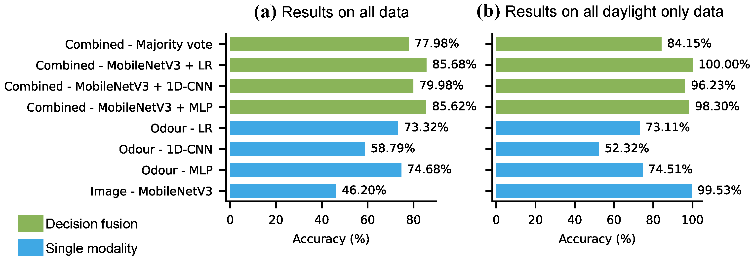
Figure 18.
Combined results of MobileNetV3 and odour models on the banana ripening data (test batch 2). Results are shown both for daylight only and all data, averaged over 25 runs.
Figure 18.
Combined results of MobileNetV3 and odour models on the banana ripening data (test batch 2). Results are shown both for daylight only and all data, averaged over 25 runs.
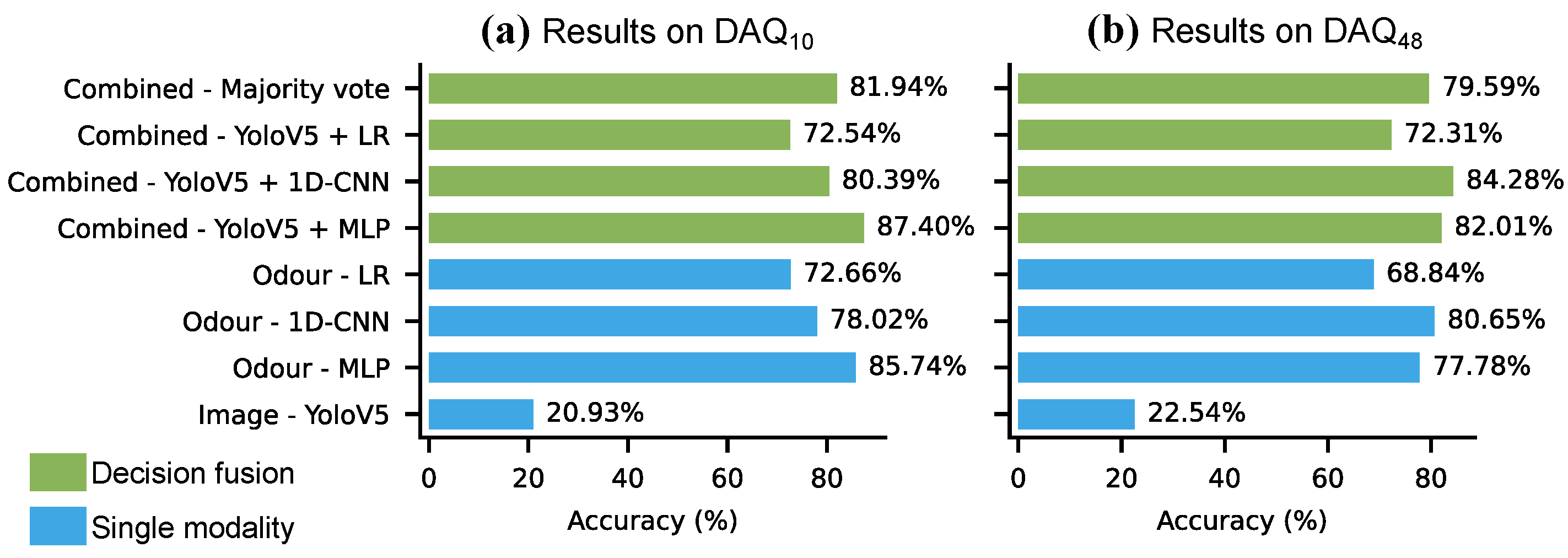
Figure 19.
Combined results of YoloV5 and odour models on the strawberry dataset. Results are shown on data from both acquisition boards on all data (both daylight and night), averaged over the 10-fold of the cross-validation results.
Figure 19.
Combined results of YoloV5 and odour models on the strawberry dataset. Results are shown on data from both acquisition boards on all data (both daylight and night), averaged over the 10-fold of the cross-validation results.
Table 1.
Related works in odour-image multimodal fusion.
Table 1.
Related works in odour-image multimodal fusion.
| Paper | Application | Sensor | Image | Fusion | Method | EN/Image/Fusion Accuracy (%) |
|---|
| [35] | Assessing mutton freshness | 10 MOX sensors (PEN3), sampling chamber type | Hyperspectral | Feature fusion | Input Modified CNN (IMCNN) | n/a (regression) |
| [36] | Beef freshness assessment | 8 QCM sensors with polymer films (KSV 5000) | Multispectral images (VideometerLab) | Decision fusion | PLSR | -/-/100.00 |
| [37] | Strawberry fungi infection identification | 10 MOX sensors (PEN3), sampling chamber type | Lab-scale visible/near-infrared HSI system | Feature fusion | SVM | n/a (regression) |
| [38] | Green vegetable identification in food | 10 MOX sensors (PEN3), sampling chamber type | Hyperspectral (camera and spectrometer) + lighting system | Data fusion | LDA | 86.37/93.28/97.50 |
| [39] | Moisture content prediction in thawed pork | 6 MOX type sensor, sampling chamber type | Hyperspectral imaging with camera, spectrometer | Decision fusion | PLSR | n/a (regression) |
| [40] | Black tea fermentation monitoring | 10 MOX sensors (PEN3), sampling chamber type | Camera + light source | Feature fusion | SVM | 86.67/82.22/95.56 |
| [41] | Tea quality identification | 10 MOX sensors (PEN3), sampling chamber type | CMOS camera | Decision fusion | SVM | 88.89/88.89/100.00 |
| [42] | Detecting freshness of spinaches | 7 MOX sensors, sampling chamber type | Camera + light source | Feature fusion | MLP | 81.25/85.42/93.75 |
| [43] | Tomato quality identification | 10 MOX sensors, sampling chamber type | CCD camera + light source | Feature fusion | SVC | 75.36/85.51/94.20 |
| [28] | Banana ripeness classification | 7 MOX type sensors and sampling chamber | CMOS camera | Feature fusion | PCA + kNN | 98.10/99.05/100.00 |
| [44] | Meat quality classification | CCS811 gas sensor in sampling chamber | CMOS camera | Feature fusion | CNN and DeepLab V3+ fused with 1D-CNN | -/-/99.44 |
| [45] | Perfume and smoke identification | 7 MOX type sensors in open-air | Thermal camera | Feature fusion | LSTM (odour) and CNN (image) | 82.00/93.00/96.00 |
Table 2.
The Figaro sensors used in the data acquisition and their sensitivity.
Table 2.
The Figaro sensors used in the data acquisition and their sensitivity.
| Numbering | Sensor | Sensitivity |
|---|
| Sensor #1 | TGS2612 | Methane, propane, iso-butane |
| Sensor #2 | TGS2611 | Methane, Natural Gas |
| Sensor #3 | TGS2602 | Air contaminants (VOCs, ammonia, H2S, etc.) |
| Sensor #4 | TGS2600 | Air contaminants (hydrogen, ethanol, etc.) |
| Sensor #5 | TGS2620 | Organic vapors (alcohol, solvent vapors) |
Table 3.
The temperature modulation patterns of applied on the heater element of the sensors, showing the sequence of voltages over time.
Table 3.
The temperature modulation patterns of applied on the heater element of the sensors, showing the sequence of voltages over time.
| | |
|---|
| Length | 5 V | 0 V | 7 V | 0 V | 5.5 V | 0 V | 5 V | 0 V | 6 V | 0 V | 6.5 V |
|---|
| 5 m | - | 30 s | 30 s | 30 s | 30 s | 30 s | 30 s | 30 s | 30 s | 30 s |
| 20 m | 30 s | 300 s | 30 s | 300 s | 30 s | 300 s | 30 s | 300 s | 30 s | 300 s |
Table 4.
Summary of the open-air dataset of ripening bananas, collected with .
Table 4.
Summary of the open-air dataset of ripening bananas, collected with .
| Data | Ripe | Overripe | All |
|---|
| Training data | 164 | 236 | 400 |
| Test data batch #1 | 40 | 48 | 88 |
| Test data batch #2 | 253 | 208 | 461 |
Table 5.
Distribution of odour samples collected in the strawberry case-study.
Table 5.
Distribution of odour samples collected in the strawberry case-study.
| Source | Ripe | Unripe | Total |
|---|
| 319 | 522 | 841 |
| 374 | 287 | 661 |
Table 6.
Summary of the RGB images collected in the strawberry case-study.
Table 6.
Summary of the RGB images collected in the strawberry case-study.
| Source | Data Shape | Number of Images |
|---|
| Camera 1-See3CAM | [2304, 1536, 3] | 1632 |
| Camera 2-HD webcamera | [1920, 1080, 3] | 1862 |
Table 7.
Mean cross-validation results on the banana ripening training data from (%).
Table 7.
Mean cross-validation results on the banana ripening training data from (%).
| Data | MLP | LR | XGB | RF | SVM | CNN | ELM | LSTM |
|---|
| 90.50 | 77.25 | 93.00 | 89.25 | 84.50 | 88.74 | 89.25 | 91.50 |
Table 8.
Mean test accuracy results (averaged over 50 runs) on the open-air banana dataset (%).
Table 8.
Mean test accuracy results (averaged over 50 runs) on the open-air banana dataset (%).
| Data | Test Batch | MLP | LR | XGB | RF | SVM | CNN | ELM | LSTM |
|---|
| 1 | 79.84 | 97.72 | 60.22 | 57.36 | 93.18 | 96.20 | 88.72 | 92.93 |
| 2 | 34.78 | 68.11 | 31.12 | 33.22 | 40.78 | 58.90 | 57.04 | 58.42 |
Table 9.
Effect of feature selection on the accuracy in the banana case-study (%), averaged over 50 runs.
Table 9.
Effect of feature selection on the accuracy in the banana case-study (%), averaged over 50 runs.
| Features | Test Batch | MLP | LR | XGB | RF | SVM | ELM |
|---|
| Small | 1 | 68.27 | 92.04 | 57.97 | 57.22 | 38.04 | 54.56 |
| Large | 1 | 79.84 | 97.72 | 60.22 | 57.36 | 93.18 | 88.72 |
| Small | 2 | 74.68 | 73.31 | 43.20 | 44.30 | 43.60 | 48.26 |
| Large | 2 | 34.78 | 68.11 | 31.12 | 33.22 | 40.78 | 57.04 |
Table 10.
Results of the 1D-CNN algorithm based on the level applied, tested on open-air banana ripening data (test batch 1). Results are averaged over 20 runs. (%).
Table 10.
Results of the 1D-CNN algorithm based on the level applied, tested on open-air banana ripening data (test batch 1). Results are averaged over 20 runs. (%).
| Accuracy (%) | Standard Deviation | Precision (%) | Recall (%) |
|---|
| Ripe | Overripe | Ripe | Overripe |
|---|
| 7 V | 60.79 | 0.0783 | 64.22 | 59.55 | 63.43 | 57.62 |
| 5.5 V | 92.38 | 0.0019 | 94.65 | 90.65 | 91.25 | 93.75 |
| 5 V | 94.94 | 0.0146 | 94.60 | 95.51 | 96.25 | 93.37 |
| 6 V | 94.26 | 0.0013 | 96.71 | 92.23 | 92.70 | 96.12 |
| 6.5 V | 96.20 | 0.0254 | 95.72 | 97.02 | 97.45 | 94.70 |
Table 11.
Mean 10-fold cross-validation accuracy results on data from the strawberry case-study (%).
Table 11.
Mean 10-fold cross-validation accuracy results on data from the strawberry case-study (%).
| | MLP | LR | XGB | RF | SVM | CNN | ELM | LSTM |
|---|
| 85.74 | 72.66 | 87.64 | 85.50 | 75.15 | 78.02 | 88.35 | 87.39 |
| 77.78 | 68.84 | 87.45 | 86.99 | 85.19 | 80.65 | 75.81 | 72.48 |
Table 12.
Mean leave-5-day-out cross-validation results (averaged over 10 runs) for the strawberry case-study (%).
Table 12.
Mean leave-5-day-out cross-validation results (averaged over 10 runs) for the strawberry case-study (%).
| Metric | Data | MLP | LR | XGB | RF | SVM | CNN | ELM | LSTM |
|---|
| Accuracy | | 76.1 | 70.9 | 75.6 | 73.7 | 87.4 | 52.0 | 82.4 | 67.0 |
| F1 | | 65.6 | 70.9 | 75.6 | 73.7 | 87.4 | 52.0 | 82.4 | 54.9 |
| Accuracy | | 72.4 | 64.6 | 72.3 | 71.3 | 75.6 | 66.8 | 61.5 | 70.4 |
| F1 | | 70.8 | 64.6 | 72.3 | 71.3 | 70.4 | 75.6 | 66.8 | 57.7 |
Table 13.
Mean 10-fold cross-validation accuracy results on data from , with and without using temperature and humidity information (%).
Table 13.
Mean 10-fold cross-validation accuracy results on data from , with and without using temperature and humidity information (%).
| | MLP | LR | XGB | RF | SVM | CNN | ELM | LSTM |
|---|
| Without | 85.74 | 72.66 | 87.64 | 85.50 | 75.15 | 78.02 | 88.35 | 87.39 |
| Features | 87.51 | 76.46 | 89.18 | 86.56 | 72.77 | n/a | 77.28 | n/a |
| Correction | 85.13 | 74.80 | 87.76 | 86.45 | 71.82 | 73.49 | 76.58 | 85.26 |
Table 14.
Mean 10-fold cross-validation accuracy results on data from the strawberry case-study (%).
Table 14.
Mean 10-fold cross-validation accuracy results on data from the strawberry case-study (%).
| | MLP | LR | XGB | RF | SVM | CNN | ELM | LSTM |
|---|
| Simple | 58.75 | 58.54 | 55.83 | 93.67 | 80.52 | 76.62 | 48.94 | 84.65 |
| Group | 47.23 | 49.09 | 59.39 | 72.10 | 64.58 | 63.72 | 47.63 | 68.01 |
Table 15.
Results of MobileNetV3 evaluated on test data batch 2 of the banana ripening case-study.
Table 15.
Results of MobileNetV3 evaluated on test data batch 2 of the banana ripening case-study.
| Test Batch | Image Subset | Accuracy (%) | Recall (%) | Precision (%) |
|---|
| | | | Ripe | Overripe | Ripe | Overripe |
|---|
| Batch 2 | All data | 46.20 | 41.50 | 51.92 | 100.00 | 99.08 |
| Daylight | 99.53 | 99.04 | 100.00 | 100.00 | 99.08 |
Table 16.
Results of YoloV5 on the strawberry data without confidence thresholding (%).
Table 16.
Results of YoloV5 on the strawberry data without confidence thresholding (%).
| | Instances | Precision | Recall | mAP50 | mAP50-95 |
|---|
| All | 6183 | 68.70 | 41.30 | 47.70 | 23.00 |
| Unripe | 2772 | 73.60 | 43.80 | 52.20 | 26.90 |
| Ripe | 3411 | 63.90 | 38.80 | 43.20 | 19.20 |
Table 17.
Results of YoloV5 on the strawberry data with confidence = 0.8 (%).
Table 17.
Results of YoloV5 on the strawberry data with confidence = 0.8 (%).
| | Instances | Precision | Recall | mAP50 | mAP50-95 |
|---|
| All | 6183 | 95.90 | 13.10 | 54.30 | 33.90 |
| Unripe | 2772 | 97.00 | 14.00 | 55.40 | 35.00 |
| Ripe | 3411 | 94.70 | 12.10 | 53.20 | 32.70 |
Table 18.
Results when binary labels (ripe/unripe) are assigned to the strawberry images.
Table 18.
Results when binary labels (ripe/unripe) are assigned to the strawberry images.
| | All Images | Subset of Well-Lit Images |
|---|
| Number of images | 1717 | 498 |
| Accuracy (%) | 26.55% | 69.07% |
| Number of images with detected objects | 533 | 361 |
| Accuracy on images with object found | 85.55% | 95.29% |
Table 19.
Accuracy of classification on the strawberry dataset where both modalities agree on the class label.
Table 19.
Accuracy of classification on the strawberry dataset where both modalities agree on the class label.
| | MLP | CNN | LR |
|---|
|
| Yolov5 and odour model agreed on % of samples (out of 841): | 18.79% (158) | 17.00% (143) | 17.48% (147) |
| When image and odour agreed accuracy was: | 98.73% | 99.30% | 97.28% |
|
| Yolov5 and odour model agreed on % of samples (out of 661): | 17.25% (114) | 17.85% (118) | 16.49% (109) |
| When image and odour agreed accuracy was: | 99.12% | 97.46% | 97.25% |